Data Envelopment Analysis and Fuzzy Theory: Efficiency Evaluation under uncertainty in portfolio optimization

Data Envelopment Analysis and Fuzzy Theory: Efficiency Evaluation

under uncertainty in portfolio optimization

Paulo Rotela Junior

1*

Edson de Oliveira Pamplona

1

Aneirson Francisco da Silva

2

Fernando Luiz Riera Salomon

1

Victor Eduardo de Mello Valerio

1

Leonardo Alves de Carvalho

1

1

Institute of Production Engineering and Management

Federal University of Itajuba

2

Department of Production

Sao Paulo State University

BPS Avenue, 1303, PO Box: 50, Itajuba-MG

BRAZIL

*

Corresponding author: [email protected]

Abstract: This article aims to analyze the behavior of a portfolio selected through Data Envelopment Analysis (DEA) associated with fuzzy logic and optimized using the Sharpe approach. As a basis for comparison, two other portfolios were used, one obtained through only the Sharpe approach. In this research study, a fuzzy DEA model was used to evaluate efficiency under uncertainty of the Brazilian Stock Exchange - Bovespa, by means of input and output indicators such as return, variance, earnings per share and price-earnings. The study reliably identified which efficient stocks and which were most sensitive to the effect of uncertainty. Through the comparison of portfolios, it was observed that the resulting combination of the fuzzy DEA models in which the stocks were considered efficient in both scenarios presented the best results.

Key-Words: Stock selection, Data Envelopment Analysis, Fuzzy Logic, Efficiency, Sharpe approach.

1 Introduction

Stock investments are a great alternative when compared to other investments, especially when observed over longer time spans. However, this higher return is accompanied by a certain level of risk. In order to maximize the return, investors must seek the best ways to invest their capital, avoiding risks larger than what they are willing to accept [1].

It is noted in recent years in Brazil that fixed income funds and savings accounts are becoming less attractive due to drop in real interest rates; the investment options that aim for better long term returns should attract investors in the coming years. Stock investments are becoming alternatives for diversification for investors seeking a long-term increase in profitability.

The first and still well-recognized model for portfolio selection was created by Markowitz [2], being a static model for evaluation of a single

period. This classic mean-variance approach is still the main model used to allocate assets and manage portfolios. It has lead to new proposals developed by academics [3-7].

For evaluation and comparison of organizational units, the technique known in the study of Operational Research as Data Envelopment Analysis (DEA), a technique developed by Charnes et al. [8], can be used to evaluate and compare organizational units that use many different inputs to produce various outputs over a specified period of time [9-11]. The concept has been amply discussed and variations on it continue to be developed.

According to Silva et al. [12], uncertain and approximate reasoning can be considered in DEA models; in order to do this, researchers use techniques related to fuzzy theory. Fuzzy DEA models are based on the model proposed by

Lertworasirikul et al. [13], a model with constant returns of scale with fuzzy coefficients.

To frame the research problem, this article aims to evaluate the efficiency of stocks of publicly traded companies through the use of fuzzy DEA models in scenarios under uncertainty.

And, as specific objectives, this article seeks to: - Utilize the Fuzzy DEA model to assist in

reducing the search space by different criteria;

- Select a portfolio with the stocks considered efficient by the Fuzzy DEA model;

- Utilize the Sharpe approach [14-15] to determine the allocation of capital in stocks considered efficient by the Fuzzy DEA model in order to minimize risk exposure to investors;

- Apply the model which incorporates the concepts of the approach proposed by Sharpe [14-15] and compare them to the other models.

2 Portfolio Selection

The basic theory of portfolio selection began with Markowitz [2], in which the selection process is based on a model of a single investment period.

The proposal of Markowitz [2] model, given by (1) - (3), is operated by Quadratic Programming techniques with the objective of portfolio optimization, taking into account the mean, variance and covariance of the expected returns of the shares, options that are to be part of the portfolio. These parameters are estimated from information of a historical series based on a mean vector and a covariance matrix of their returns.

1 1

minZ

.

cov

n n i j ij i j

x x

= =

=

∑∑

(1) Subject to:

*

) ( 1

E

E

x

_ri j i i

=

∑

= (2)

1

1

=

∑

= j i i

x

(3)

Where xi and xj represent the percentage share of the asset i and stock j in the optimal portfolio, E (ri) is the expected return stock i, i = 1 a j, and E * is the expected return of the portfolio.

Sharpe [14] extended the work of Markowitz [2]. He introduced a simplified model of the relationships between assets that offered evidence of

costs [16]. It was also convenient to use the model for practical applications, as in equations (4)-(6) [2]:

1 1 2 1 1

maxZ

N N i i i i i i

X A

X Q

λ

+ + = =

=

∑

−

∑

(4)

Which is subjected to:

X

_i≥ 0 for each

i from 1 to N. 1 N i i n i i

X B

X

₊ =

=

∑

(5) 1

1

N i i

X

=

=

∑

(6)

This formula shows why parameters An+1 and

Qn+1 are used to describe variance and the future

expected value of I. This fact also shows why this is called the diagonal model. The variance and covariance model, which is complete when N assets are considered, can be expressed as a matrix with non-zero values on the diagonal, including an (n+1)th asset defined as has been shown [14]. This drastically reduces the number of calculations needed to solve the portfolio analysis problem. It allows the problem to be recognized directly in terms of the parameters of the diagonal model.

According to Ben Abdelaziz et al. [17], the mean-variance methodology proposed by Markowitz [2] for portfolio selection has been essential for the activity of research and has served as the basis for the development of modern financial theory.

In the literature, some algorithms, such as those proposed by Sharpe [8], were created in order to linearize and improve the efficiency of the covariance Markowitz [1, 16, 18-19]. However, researchers have developed more sophisticated models that use multi-period or dynamic extensions, in which the association between data envelopment analysis and fuzzy logic can be an alternative, like the model presented below.

3 Data Envelopment Analysis

associated to Fuzzy Logic

The main purpose of Data Envelopment Analysis (DEA) is to evaluate the efficiency of productive units which perform similar tasks, called decision-making units (DMUs). These units are compared to each other and are differentiated by amounts of resources (inputs) they consume and the goods (outputs) they produce [15, 20-22].

DEA models allow more than simple analysis of the DMUs that can be classified as efficient; they also allow one to measure and locate the

inefficiency and estimate a linear production function that provides the benchmark for the DMUs classified as ineffective. This benchmark can be established by the projection of inefficient DMUs on the efficiency frontier [22].

For Kao [11] and Silva et al. [12], DEA enables the identification of DMUs that are references (benchmark) for the identification of other decision making units under analysis.

Authors as Bal et al. [23] and Rotela et al. [1] show that DEA has stood out among the realm of quantitative modeling techniques which aid decision making, assisting managers from various fields, such as banks, schools, and hospitals [11, 21, 24-25]. Charnes, Cooper and Rhodes [8] developed the first DEA model to evaluate the effectiveness of public programs.

Cooper et al. [20] assert that the input and output variables for each DMU should be chosen to represent the interest of managers, and there must be positive numeric data for each input and output, and it is preferable to use a smaller number of inputs compared to the outputs. Outlined below are the classical DEA models: CCR and BCC.

According to Malekmohammadi et al. [26] and Miranda et al. [27], the first, known as the DEA CCR model, or model with constant returns of scale, proposed by Charnes et al. [8] as (7) - (11):

0 1

max

.

s o r r r

w

u y

=

=

∑

(7) Subject to:

1

1

=

∑

= io m i i

x

v

(8)

∑

∑

= =

=

≤

−

s r io m i i r r

y

v

x

j

n

u

1 1 0

0

1

,

2

,....,

(9)

.

,...,

2

,

1

,

0

r

s

u

_r

≥

=

(10)

.

,...,

2

,

1

,

0

i

m

v

_i

≥

=

(11)

In which j represents the index of the DMU, j = 1, ..., n; r is the output index, with r = 1, ..., s; i is the input index, i = 1, ..., m; yrj is the value of the r

-th output for the j-th DMU; xij is the value of the ith input to the jth DMU; ur is the weight associated with the r-th output; vi is the weight associated to the ith input; wo is the relative efficiency of DMUo,

which is the DMU under evaluation; and yr0 and xio are the technology coefficients of data arrays for inputs and outputs, respectively [27].

When wo = 1, this indicates that DMU0, under

analysis, shall be considered efficient when

compared to the other units included in the model. If wo < 1, this should be considered an inefficient DMU [28].

Banker et al. [29] transformed the assumption of constant returns to scale in the CCR model through a restriction of convexity, creating the DEA-BCC model that admits variable returns of scale, as seen in (12) - (16): 0 0 1

max

.

s o r r r

w

u y

c

=

=

∑

+

(12) Subject to:

1

1

=

∑

= io m i i

x

v

(13)

∑

∑

= =

=

≤

+

−

s r io m i i r r

y

v

x

c

j

n

u

1 0 1 0

0

1

,

2

,....,

(14)

.

,...,

2

,

1

,

0

r

s

u

_r

≥

=

(15) . ,..., 2 , 1 , 0 i m vi ≥ = (16)

It is worth noting that to obtain the formulation of the DEA-BCC model, an unrestricted auxiliary variable c0, known as a scale factor, was inserted

additively in equations (12) and (14).

Kao and Liu [30] develop a method to find the membership functions of the fuzzy efficiency scores when some observations are fuzzy numbers [31].

According to the definition provided by Lertworasirikul et al. [13], Fuzzy Data Envelopment Analysis (FDEA or Fuzzy DEA) is a tool to compare the performance of a set of activities or organizations under uncertain environment. Inaccurate data in FDEA models are represented by fuzzy sets and FDEA models can take the form of fuzzy linear programming models. The FDEA models may be more realistic than models representing real envelopment analysis of conventional data problems. However, there are some FDEA models that do not use fuzzy linear programming; such models are based on the concepts of upper and lower frontiers [32-33].

In their research, Hatami-Marbini et al. [34] cite four major approaches that deal with the fuzzy DEA models: The tolerance approach; the α-level based approach; the Fuzzy ranking approach; and the Possibility approach.

Hatami-Marbini et al. [34] and other authors such as Silva et al. [12] and Wen and Li [31], believe that the α-level approach is the most commonly used FDEA model, and is also the approach proposed by Kao and Liu [30].

According to Chen et al. [35], when assessing risk characteristics and estimating efficiency, it is appropriate to use the FDEA model, where inputs and outputs are non-specific values.

Hatami-Marbini et al. [34] and Miranda et al. [27] state that many researchers have formulated FDEA models to deal with situations that present imprecise or vague data input and output.

The FDEA BCC model, which admits variable returns of scale, is shown in (17) - (21):

~ ~ 0 0 max j _r. _r r R E u y c ∈ +

∑

(17) Subject to: ~

1

io i i I

v x

∈

=

∑

(18) ~ ~ 0 0 rj r i ij r R i I u Y v X c j J ∈ ∈ − + ≤ ∀ ∈

∑

∑

(19) 0, r R r u ≥ ∀ ∈ (20) 0, i v ≥ ∀ ∈i I (21)

Where, according to Silva et al. [12], DMU0 is

being analyzed;

~ 0

i

x are the fuzzy variables of the i-th entry of DMU0;

~ 0

r

y are the fuzzy variables of the r-th output of DMU0;

~

ij

X

represents the matrix of

fuzzy variables of the i-th input of the DMU j; represents the matrix of fuzzy variables of r-th output DMU j.

The objective function (17) may have a greater value than 1 due to constraints (18) and (19) which involve Fuzzy parameters and are solved using probability [7, 20].

In this article, will be adopted the Hatami-Marbini et al [34] α-level based approach. The α Є [0, 1] value allows to generate different scenarios, i.e., different values of efficiency, respecting the variation range determined by the pertinence function [12].

Based on the α-level approach, according to Silva et al. [12], when the value of α = 0, the parameter values are below average; that is, they will approach the lower limit value of the pertinence function. However, when the parameter value is above average, it will be exactly the values of the upper limit of the pertinence function.

Yet according to the same authors, when the value of α = 1, there is a scenario in which the

values of output parameters and input data are formed by the average of the pertinence function, then considering the most probable values; that is, a scenario that ignores uncertainty.

For this, in this research were considered two FDEA-BCC models used by Miranda et al. [28]. These two models, resulting from the Banker et al. [29] and Kao e Liu [30] approaches, analyses pessimist (22)-(26) and optimistic scenarios, accordingly (27)-(30), where c0 is unrestricted:

~ 0 0 0 max j _r.(Y_{r r} ) r R E u

ρ α

c ∈ − ⋅ +

∑

(22) Subject to: ~

(

) 1

i io io i I

v x

α

∈

+ Ψ ⋅

=

∑

(23) ~ ( ) r rj rj r R u Y

ρ α

∈ − ⋅ −

∑

~ 0 ( ) 0 i ij ij i I v X

α

c j J ∈ + Ψ ⋅ + ≤ ∀ ∈

∑

(24) 0, r R r u ≥ ∀ ∈ (25) 0, i v ≥ ∀ ∈i I (26) ~ 0 0 0 max j _r.( _{r r} ) r R E u y

ρ α

c ∈ + ⋅ +

∑

(27) Subject to: ~

(X

) 1

i io io i I

v

α

∈

− Ψ ⋅

=

∑

(28) ~ ( ) r rj rj r R u y

ρ α

∈ + ⋅ −

∑

~ 0 ( ) 0 i ij ij i I v X

α

c j J ∈ − Ψ ⋅ + ≤ ∀ ∈

∑

(29) 0, r R r u ≥ ∀ ∈ (30) 0, i v ≥ ∀ ∈i I (31)

Where, according to Miranda et al. [27], α is the value chosen for the α-level based approach, with variation [0, 1]; Ψio is the α coefficient in constraints linked to the i-th Fuzzy input for DMU0; ρrj is the α coefficient in constraints linked to the j-th Fuzzy output for DMU0; ρj0 is the α coefficient for constraints linked to the r-th Fuzzy output of the j-th DMU; and Ψij is the α coefficient for constraints linked to the i-th Fuzzy input of the j-th DMU.

4 Materials and Methods

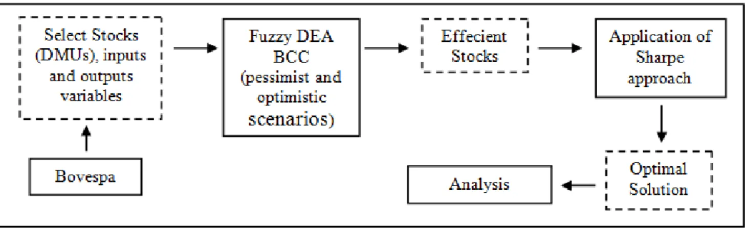
This research uses the scientific basis developed by Markowitz [2] and Sharpe [14] to present a method for selecting stock portfolios. To select assets considered efficient Fuzzy DEA model will be used, as described in Figure 1.

Figure 1: Research flowchart

The initial sample was composed of stocks of publicly traded companies negotiated on the São Paulo Stock Exchange (Bovespa), obtained by consulting the database Economática® software.

Initially, the set of inputs and outputs to be used in the analysis of efficiency by DEA model were determined.

Authors such as Powers and McMullen [36], and Lopes et al. [37] used indicators with returns after one, two and three years and earnings per share to compose the set of outputs while Beta (60 months), price-earnings and volatility (36 months) to compose the inputs of the DEA model indicators. However, Rotela et al. [1] proposed replacing the indicators that make up the inputs for volatility in windows of 12 months over years 1, 2 and 3, along with price-earnings. This change in the risk measurement indicator set can provide information that will allow the DEA model to choose assets that are comparatively analyzed and found to be efficient [1]. They treated attributes with advantages as outputs and those with costs as inputs for the model.

24 companies with the largest participation in Bovespa were selected for consideration, regardless of their classification as either common or preferred stocks. The sample could have been greater, but the minimum number was selected to meet the requirement of DEA with respect to the number of DMUs, considering using eight indicators, four for input and four for output.

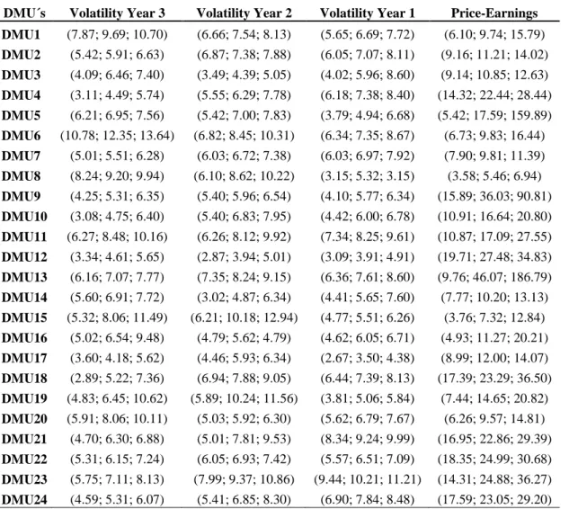
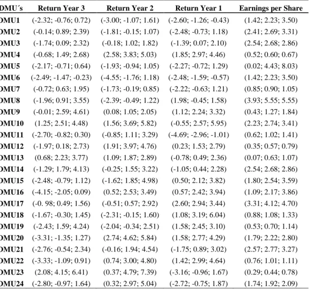
Data were collected using Economática ® software during the period from April 2011 to March 2014. For each of the input and output variables, the minimum, average and maximum values obtained in the period were identified. This article aims to evaluate the effectiveness of assets (DMUs), in which the inputs were considered indicators aiming to minimize, as shown in Table 1. The outputs, indicators to be maximized, are shown in Table 2.

Table 1: Triangular pertinence functions for inputs

Table 2: Triangular pertinence functions for outputs

Triangular pertinence functions were used to insert uncertainty in the input parameters (inputs) and output (outputs) of the FDEA model. According to authors such as Silva et al. [12], Liang and Wang [38] and Aouni et al. [39] they represent human expertise to correctly judge the behavior of variables common in many practical situations.

It is noteworthy that the negative data were treated as proposed by Cook and Zhu [40], which adds the value that makes the most negative value positive, without changing the model analysis Fuzzy DEA. For modeling the FDEA model, the software General Algebric Modeling (GAMS ®), version 23.6.5 and CPLEX solver in version 12.2.1 were used.

With the purpose of comparison, three portfolios were proposed. Then, the monthly returns of the past 36 months for each of the assets were utilized. Data were collected with the aid of Economática ® software and treated in order to avoid the presence of outliers.

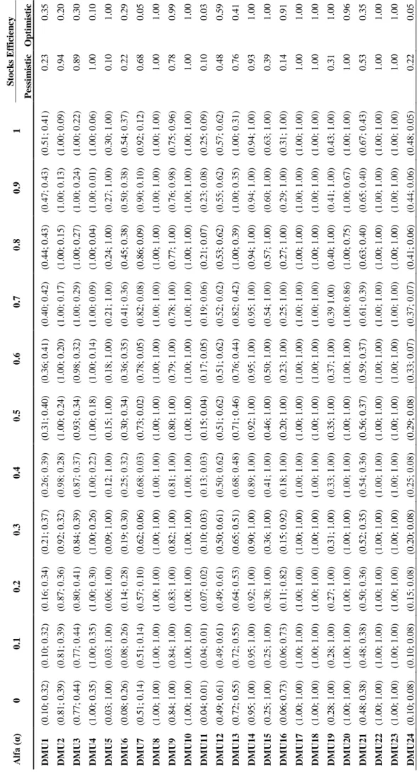
Efficiency results based on the α-level are presented in Table 3. The values in parentheses represent the pessimistic and optimistic scenario, respectively, for the values for each DMU.

In the articles proposed by Kao and Liu [11] and Miranda et al. [27], the authors use the geometric mean between the optimistic and pessimistic DEA approaches to establish an index of overall risk, as is also proposed by Fare et al. [41] and Chin et al. [42]. The geometric mean of the results presented by the α-level was used, then obtaining in Table 3, where the efficiency for each of the scenarios is given.

Through analysis of Table 3, it is noted that only six stocks were efficient in both scenarios. These assets considered efficient in both scenarios were used in assembling the portfolio denominated FDEA-6. However, to put together the portfolio denominated FDEA-11, all the stocks considered efficient in at least the optimistic or pessimistic scenario were aggregated. This portfolio consists of 11 stocks.

Table 3: Efficiency values in α-level functions

In both portfolios, after the implementation of the fuzzy DEA model, the Solver add-in for Microsoft Excel ® was used to optimize the model through the Sharpe approach for the stocks considered efficient. Then the recommended weights for each of the stocks comprising the portfolios were determined.

Finally, a third portfolio, called the comparative portfolio (Cp), in which only Solver was used in Microsoft Excel to optimize the 24 stocks through the Sharpe Ratio approach, obtaining the recommended weight for each stocks. It is noteworthy that there was no pre-selection through FDEA modeling.

Later, has begun the process of verifying the existence of abnormal returns. For this, it was used the Capital Asset Pricing Model (CAPM) methodology, proposed by Sharpe [15], in which it was possible to compare the portfolio in relation with expected return.

To identify abnormal returns for the assets of each portfolio, it was calculated the difference between the expected return and return provided by the CAPM observed during the analysis period.

By using the CAPM, in addition to obtaining the rate of return, could be quantified the relationship between risk and return for which the company’s stocks are subject [15]. Already about risk, the CAPM consists of two pillars, the diversifiable or unsystematic risk and un-diversifiable or systematic risk.

In CAPM equation, for the risk-free rate (Rf), it was applied the Special System of Clearance and Custody (Selic) average rate during the period from April 2010 and March 2014, for being considered an indicator of basic interest rate of the economy of the Brazilian Federal Treasury.

In reviewing the performance of the expected return of the market (Rm), it was observed the behavior of Bovespa Index from the beginning of 1995 to the first quarter of 2014. Expected return of the market was then calculated based on the average of the observed years.

Discounted the inflation rate, it was used value of 5.1% p.a. for Selic average rate and 10.80% p.a. for (Rm) in the definition of the expected return of portfolios.

Next, it was calculated the Beta (β) term, in which, for each of the three portfolios formulated, was calculated using the weighted average of the individual Beta multiplied by the percentage of each stock. For this, there was obtained the individual Beta for each asset with the aid of Economática ® software, during the same period used for the monthly returns. Finally, could be possible to verify if the portfolios resulted in returns above expected.

For a more complete analysis, was also used the Sharpe Ratio (SR), which, according Rotela et al. [1], Schuhmachera and Elingb [43] and Schuster and Benjamin [44] is a measure of efficiency in the use of risk to generate returns. The SR establishes a relationship between the excess return of a given

investment portfolio relative to the risk-free rate and investment risk. Selic average in the previously proposed period was assumed as risk-free rate, and standard deviation of monthly returns of portfolios as risk measure.

5 Results and Analysis

The result was the formation of three portfolios, one using only the Sharpe approach called comparative portfolio (Cp), and two resulting from a selection of stocks considered efficient using the FDEA model. It is noteworthy that after selection with the FDEA model, the Sharpe approach was used to determine capital allocation for each stock. The goal was to build a portfolio without significant additional risks, viewed as a portfolio with superior performance; that is, with a ratio of return and risk better than the optimized portfolio with only the Sharpe model (Cp).

Applying only the Sharpe approach in the list of 24 stocks with the largest holdings in the Bovespa Index, the comparative portfolio (Cp) was obtained consisting of 13 stocks.

In assembling the portfolio FDEA-11, an evaluation of the efficiency of the 24 stocks (DMUs) was performed, and eleven were considered efficient in at least one of the scenarios. The Sharpe approach was applied and only five such assets composing the portfolio were obtained.

Finally, to select the FDEA-6 portfolio, an efficiency analysis of the initial sample was performed and only six stocks (DMUs) were considered effective in both the optimistic scenario and pessimistic scenario. The Sharpe approach was again applied to identify the optimal allocation of resources, and finally obtained the FDEA-6 portfolio, composed of only four stocks, as shown in Table 4.

Table 4: Asset allocation

It is important to note that all four stocks used in assembling the portfolio FDEA-6 are part of the portfolio FDEA-11, which can be expected, since it is composed of assets that were efficient in both scenarios. However, it is interesting to note that the same assets are also part of the group used in the composition of the comparative portfolio (Cp).

As in the work from Rotela et al. [1], as the focus of optimization was to obtain efficient stocks using the risk measured by variance in similar periods as input variables, price-earnings ratio, and as output variables the monthly index return and earnings per share, it is believed that the assets considered

efficient showed good relationships between the indicators in the period, positively impacting the result.

Table 5 shows the standard deviation results, return and Sharpe Ratio (SR), obtained with the proposed portfolios. Comparing the results obtained by the SR, it can be seen that the comparative portfolio (Cp) showed positive SI of 2.59. On the other portfolio FDEA-11 showed an SR of 2.93. And finally for the FDEA-6 portfolio in which the efficiency was evaluated for the 24 initially proposed stocks and six were considered efficient. Then these were optimized by the Sharpe approach, obtaining the participation of each of the stock in order to maximize the SR. The optimized portfolio showed an SR of 3.12, showing that the risk offering is rewarded, even surpassing the results of other portfolios, being an attractive investment.

Table 5: Results Table

Performing a comparison between the values obtained in each SR portfolios, one can observe the outperformance of portfolio FDEA-6 over the others, in which an investor could earn a higher premium for the risk assumed.

It can be seen, in Table 5, that the expected return of the three portfolios are near from each other, where the portfolio (Cp) presents (0.58%), FDEA-11 (0.59%) and FDEA-6 (0.59%) per month.

The return effectively earned by portfolios (Cp) (1.78%), FDEA-11 (2.93%) and FDEA-6 (1.98%), per month, demonstrate the existence of abnormal returns compared with their expected returns obtained by CAPM.

The observed risk measured by the standard deviation, as can be seen in Table 5, was virtually identical in both portfolios put together through the FDEA model, as in the comparative portfolio (Cp). However, the average monthly return surpassed the comparative profitability of the portfolio, formed only with the aid of the proposed Sharpe, demonstrating a better return on risk ratio for portfolios using the DEA model associated with the fuzzy approach. Another benefit that can be cited is the reduced number of stocks comprising the portfolio FDEA-6, which may ultimately produce savings related to the cost of re-balancing the portfolio.

The data from the 36 months used in the study were obtained from the accumulated portfolios (Cp), FDEA-11, FDEA-6, and the Bovespa Index return over the same period. Thus, it was possible to observe that the portfolios outperform the Bovespa Index, as shown in Figure 2. Optimized portfolio

FDEA-6 gets the best performance, with a cumulative return of 102.14%, followed by portfolio FDEA-11, which presents a cumulative return of 98.25%. The portfolio (Cp) has a cumulative return of 41.32% in the period.

Figure 2: Return accumulated per portfolio

Another advantage to be mentioned is that a purely deterministic model was not used; instead, stocks were selected according to their efficiency through multiple criteria, not just risk and return, and considering the uncertainty and imprecision, thus providing a more robust analysis.

6 Conclusions

This article aimed to evaluate the feasibility and viability of using data envelopment analysis associated with fuzzy logic in order to select a portfolio and then optimize its equity. For this purpose, three portfolios were proposed: the first simply by using an optimized Sharpe approach and the other two using fuzzy logic associated with the DEA.

Several studies, not only with the use of DEA as well as other mathematical models, treat the case as deterministic, being accurate in its determination of the input and output variables. However, it is known that in practice, real world problems are naturally uncertain and imprecise.

The goal was to obtain a model that considered uncertainty and imprecision, and still presented a better ratio of risk/ return, however, without leading to a sharp increase in the variance.

The application of fuzzy DEA models was feasible, providing an excellent breakdown of the analysis units. It is worth noting that the fuzzy DEA model assists in reducing the search space, since it determines which assets should be considered efficient through various scenarios by reducing the number of stocks that will be submitted to the Sharpe approach, for example.

The well-recognized Sharpe approach proves to be efficient in its objective; however, its practical use can be difficult and even engaged in some situations, since one obtains a large number of assets composing the portfolio holdings and impossible to be performed.

Another benefit to be cited is the reduced number of stocks comprising the FDEA-6 portfolio. Such reduction associated with the maintenance of the level of risk under control tends to generate savings related to the cost of re-balancing portfolios, providing indirect investor gains.

Data Envelopment Analysis is already considered to be part of a set of techniques that assist in selecting assets for portfolio composition. Moreover, the combination of the FDEA approach can further assist in portfolio composition. The association of the FDEA approach with Sharpe has been successful, and two main advantages can be cited: a larger number of variables was used in the analysis to make it more robust, which may accommodate different indicators; As a result, a reduced number of stocks composing the portfolio was obtained, which makes its use possible and gave the best SR between the portfolios analyzed.

As a suggestion for further research, the use of other indicators and a long-term analysis are suggested. It is also recommended that a more comprehensive study using a greater number of stocks to check whether the model would replicate the results obtained in this study.

References:

[1] P. Rotela Junior, E. O. Pamplona and F. R. Salomon. Portfolio optimization: efficiency analysis, RAE, v. 54, n. 4, 2014.

[2] H. Markowitz. Portfolio selection, Journal of Finance, v. 7, n. 1, p. 77-91, 1952.

[3] T. Cover and D. Julian. Performance of universal portfolios in the stock market: information theory, Proceedings of IEEE International Symposium on Information Theory, Sorrento, p. 232, 2000.

[4] J. Tu and G. Zhou. Markowitz meets Talmud: A combination of sophisticated and naive diversification strategies. Omega, v. 28, p. 385-398, 2000.

[5] J. Brodie, I. Daubechies, C. Mol, D. Giannone and I. Loris. Sparce and stable Markowitz portfolios. Proceedings of the National Academy of Sciences of the United States of America, v. 106. n. 30, 2009.

[6] F. Ditraglia, J. Gerlach. Portfolio selection: An extreme value approach. Journal of Banking & Finance, v. 37, n. 2, p. 305-323, 2013.

[7] C. Zopounidis, M. Doumpos, F. Fabozzi. Preface to the Special Issue: 60 years following Harry Markowitz’s contributions in portfolio theory and operations research. European Journal of Operational Research, v. 234, n. 2, p. 343-345, 2014.

[8] A. Charnes, W. Cooper and E. Rhodes. Measuring the efficiency of decision-making units, European Journal of Operational Research, v. 2, n. 6, p. 429-444, 1978.

[9] L. Kuo, S. Huang, Y. Wu. Operational efficiency integratingthe evaluation of environmental investment: the case of Japan. Management Decision, v. 48, n. 10, p. 1596– 1616, 2010.

[10]A. Amirteirmoori. A DEA two-stage decision processes with shared resources. Central European Journal of Operations Research, v. 21, p. 141-151, 2011.

[11]C. Kao and S. Liu. Multi-period efficiency measurement in data envelopment analysis: The case of Taiwanese commercial banks. Omega, v. 47, p. 90-98, 2014.

[12]A. F. Silva, F. A. Marins and M. V. Santos. Goal Programming and Data Envelopment Analysis combined with Fuzzy Theory to evaluate efficiency under uncertainty: application in mini-factories of the auto parts segment, Gestão & Produção, ahead of print,

São Carlos, 2014,

http://dx.doi.org/10.1590/S0104-530X2014005000012.

[13]S. Lertworasirikul, S. Fang, J. Joines and H. Nuttle. Fuzzy Data Envelopment Analysis (DEA): A possibility approach, Fuzzy Sets and Systems, v. 139, 2003.

[14]W. F. Sharpe. A simplified model for portfolio analysis, Management Science, n. 9, 1963. [15]W. F. Sharpe. Capital Assets prices: A Theory

of Market Equilibrium under conditions of Risk, Journal of Finance, v. 19, 1964.

[16]S. Darolles and C. Gourieroux. Conditionally fitted Sharpe performance with an application to hedge fund rating. Journal of Banking & Finance, v. 34, p. 578-593, 2010.

[17]F. Ben Abdelaziz, B. Aouni, R. El Fayedh. Multi-objective stochastic programming for portfolio selection, European Journal of Operational Research, v. 177, n. 3, 2007.

[18]D. N. Nawrocki and W. L. Carter. Earnings announcements and portfolio selection. Do they add value?, International Review of Financial Analysis, n. 7, 1998.

[19]C. Shing and H. Nagasawa. Interactive decision system in stochastic multi-objective portfolio selection, International Journal of Production Economics, v. 60, 1999.

[20]W. Cooper, L. Seiford and K. Tone. Data envelopment analysis: a comprehensive text with models, application, references and DEA-Solver Software, 2nd. ed. New York: Springer Science + Business, 2007.

[21]L-J. Kao, C-J. Lu and C-C Chiu. Efficiency measurement using independent component analysis and data envelopment analysis.

European Journal of Operational Research, v. 210, p. 310–317, 2011.

[22]W. Cook and J. Zhu. Data Envelopment Analysis – A Handbook on the modeling of internal structures and networks. New York: Springer Science + Business, 2014.

[23]H. Bal, H. Orkcu and S. Çelebioglu. Improving the discrimination power and weights dispersion in the data envelopment analysis, Computer & Industrial Engineering, v. 37. n. 1, 2010.

[24]P. Bachiller. Effect of ownership on efficiency in Spanish companies. Management Decision, v. 47. n. 2, p. 289-307, 2009.

[25]J. Liu, L Lu, W-M. Lu and B. Lin. A survey of DEA applications. Omega, v. 41, n. 5, p. 893– 902, 2013.

[26]N. Malekmohammadi, F. Lotfi and A. Jaafar. Data envelopment scenario analysis with imprecise data. Central European Journal of Operations Research, v. 19, p. 65-79, 2009. [27]R. C. Miranda, J. A. B. Montevechi, A. F. Silva

and F. A. Marins. A new approach to reducing search space and increasing efficiency in simulation optimization problems via the Fuzzy-DEA-BCC, Mathematical Problems in Engineering, Volume 2014, Article ID 450367, 2014.

[28]J. Jablonsky. Multicriteria approaches for ranking of efficient units in DEA models. Central European Journal of Operations Research, v. 20, p. 435-449, 2012.

[29]R. Banker, A. Charnes and W. Cooper. Some models for estimating technical and scale inefficiencies in Data Envelopment Analysis, Management Science, v. 30, n. 9, 1984.

[30]C. Kao and S. Liu. Fuzzy efficiency measures in data envelopment analysis, Fuzzy Sets and Systems, v. 133, 2000.

[31]M. Wen and H. Li. Fuzzy data envelopment analysis (DEA): Model and ranking method, Journal of Computational and Applied Mathematics, v. 223, n. 2, 2009.

[32]D. Despostis and Y. Smirlis. Data Envelopment Analysis with Imprecise Data, European Journal of Operational Research, v. 140, n. 1, 2002.

[33]L. Biondi Neto, J. Mello, L Meza, E. Gomes and N Bergiante. A geometrical approach for Fuzzy DEA frontiers using different T norms, WSEAS Transactions on Systems, v. 10, n. 5, p. 127-136, 2011.

[34]A. Hatami-Marbini, A. Emrouznejad and M. Tavana. Taxonomy and review of the Fuzzy Data Envelopment Analysis literature: two

decades in the making, European Journal of Operational Research, v. 214, 2011.

[35]Y-C. Chen , Y-H. Chiu, C-W. Huang and C-H. Tu. The analysis of bank business performance and market risk—Applying Fuzzy DEA, Economic Modelling, v. 32, p. 225-232, 2013. [36]J. Powers and P. McMullen. Using data

envelopment analysis to select efficient large market cap securities, Journal of Business and Management, v. 7, n. 2, p. 31-42, 2000.

[37]A. L. Lopes, M. Carneiro and A. Schneider. Markowitz na otimização de carteiras selecionadas por Data Envelopment Analysis – DEA, Revista Gestão e Sociedade, v. 4, n. 9, 640-656, 2010.

[38]G. Liang and M. Wang. Evaluating human reliability using Fuzzy Relation, Microelectronics Reliability, v. 33, n. 1, 1993. [39]B. Aouni, J. Martel and A. Hassaine. Fuzzy

Goal Programming Model: An overview of the current state of the art, Journal of Multi-Criteria Decision Analysis, v. 16. n. 5, 2009. [40]W. Cook and J. Zhu. Data envelopment

analysis: modeling operational processes and measuring productivity. Worcester: Create Space Independent Publishing Platform, 2008. [41]R. Färe, S. Grosskopf, M. Norris and Z. Zhang.

Productivity growth, technical progress and efficiency change in industrialized countries, American Economic Review, n. 84, p. 66–83, 1994.

[42]K-S. Chin, Y-M. Wang, G. Poon and J-B. Yang. Failure mode and effects analysis using a group-based evidential reasoning, Computers & Operations Research, v. 36, n. 6, p. 1768-1779, 2009.

[43]F. Schuhmacher and M. Eling. Sufficient conditions for expected utility to imply drawdown-based performance rankings, Journal of Banking and Finance, v. 35, n. 9, p. 2311-2318, 2011.

[44]M. Schuster and A. Benjamin. A note on empirical Sharpe Ratio dynamics, Economic Letters, v. 116, n. 1, p. 124-128, 2012.

ACKNOWLEDGMENTS

The authors would like to express their gratitude to the Brazilian agencies CNPq (National Counsel of Technological and Scientific Development), CAPES (Post-Graduate Federal Agency), and FAPEMIG (Foundation for the Promotion of Science of the State of Minas Gerais), which have been supporting the efforts for the development of this work in different ways and periods.

Table 1: Triangular pertinence functions for inputs

DMU´s Volatility Year 3 Volatility Year 2 Volatility Year 1 Price-Earnings DMU1 (7.87; 9.69; 10.70) (6.66; 7.54; 8.13) (5.65; 6.69; 7.72) (6.10; 9.74; 15.79) DMU2 (5.42; 5.91; 6.63) (6.87; 7.38; 7.88) (6.05; 7.07; 8.11) (9.16; 11.21; 14.02) DMU3 (4.09; 6.46; 7.40) (3.49; 4.39; 5.05) (4.02; 5.96; 8.60) (9.14; 10.85; 12.63) DMU4 (3.11; 4.49; 5.74) (5.55; 6.29; 7.78) (6.18; 7.38; 8.40) (14.32; 22.44; 28.44) DMU5 (6.21; 6.95; 7.56) (5.42; 7.00; 7.83) (3.79; 4.94; 6.68) (5.42; 17.59; 159.89) DMU6 (10.78; 12.35; 13.64) (6.82; 8.45; 10.31) (6.34; 7.35; 8.67) (6.73; 9.83; 16.44) DMU7 (5.01; 5.51; 6.28) (6.03; 6.72; 7.38) (6.03; 6.97; 7.92) (7.90; 9.81; 11.39) DMU8 (8.24; 9.20; 9.94) (6.10; 8.62; 10.22) (3.15; 5.32; 3.15) (3.58; 5.46; 6.94) DMU9 (4.25; 5.31; 6.35) (5.40; 5.96; 6.54) (4.10; 5.77; 6.34) (15.89; 36.03; 90.81) DMU10 (3.08; 4.75; 6.40) (5.40; 6.83; 7.95) (4.42; 6.00; 6.78) (10.91; 16.64; 20.80) DMU11 (6.27; 8.48; 10.16) (6.26; 8.12; 9.92) (7.34; 8.25; 9.61) (10.87; 17.09; 27.55) DMU12 (3.34; 4.61; 5.65) (2.87; 3.94; 5.01) (3.09; 3.91; 4.91) (19.71; 27.48; 34.83) DMU13 (6.16; 7.07; 7.77) (7.35; 8.24; 9.15) (6.36; 7.61; 8.60) (9.76; 46.07; 186.79) DMU14 (5.60; 6.91; 7.72) (3.02; 4.87; 6.34) (4.41; 5.65; 7.60) (7.77; 10.20; 13.13) DMU15 (5.32; 8.06; 11.49) (6.21; 10.18; 12.94) (4.77; 5.51; 6.26) (3.76; 7.32; 12.84) DMU16 (5.02; 6.54; 9.48) (4.79; 5.62; 4.79) (4.62; 6.05; 6.71) (4.93; 11.27; 20.21) DMU17 (3.60; 4.18; 5.62) (4.46; 5.93; 6.34) (2.67; 3.50; 4.38) (8.99; 12.00; 14.07) DMU18 (2.89; 5.22; 7.36) (6.94; 7.88; 9.05) (6.44; 7.39; 8.13) (17.39; 23.29; 36.50) DMU19 (4.83; 6.45; 10.62) (5.89; 10.24; 11.56) (3.81; 5.06; 5.84) (7.44; 14.65; 20.82) DMU20 (5.91; 8.06; 10.11) (5.03; 5.92; 6.30) (5.62; 6.79; 7.67) (6.26; 9.57; 14.81) DMU21 (4.70; 6.30; 6.88) (5.01; 7.81; 9.53) (8.34; 9.24; 9.99) (16.95; 22.86; 29.39) DMU22 (5.31; 6.15; 7.24) (6.05; 6.93; 7.42) (5.57; 6.51; 7.09) (18.35; 24.99; 30.68) DMU23 (5.75; 7.11; 8.13) (7.99; 9.37; 10.86) (9.44; 10.21; 11.21) (14.31; 24.88; 36.27) DMU24 (4.59; 5.31; 6.07) (5.41; 6.85; 8.30) (6.90; 7.84; 8.48) (17.59; 23.05; 29.20)

Table 2: Triangular pertinence functions for outputs

DMU´s Return Year 3 Return Year 2 Return Year 1 Earnings per Share DMU1 (-2.32; -0.76; 0.72) (-3.00; -1.07; 1.61) (-2.60; -1.26; -0.43) (1.42; 2.23; 3.50) DMU2 (-0.14; 0.89; 2.39) (-1.81; -0.15; 1.07) (-2.48; -0.73; 1.18) (2.41; 2.69; 3.31) DMU3 (-1.74; 0.09; 2.32) (-0.18; 1.02; 1.82) (-1.39; 0.07; 2.10) (2.54; 2.68; 2.86) DMU4 (-0.68; 1.49; 2.68) (2.58; 3.83; 5.03) (1.85; 2.97; 4.46) (0.52; 0.60; 0.67) DMU5 (-2.17; -0.71; 0.64) (-1.93; -0.94; 1.05) (-2.27; -0.72; 1.29) (0.02; 4.43; 8.03) DMU6 (-2.49; -1.47; -0.23) (-4.55; -1.76; 1.18) (-2.48; -1.59; -0.57) (1.42; 2.23; 3.50) DMU7 (-0.72; 0.63; 1.95) (-1.73; -0.19; 0.85) (-2.22; -0.63; 1.21) (0.85; 0.90; 1.05) DMU8 (-1.96; 0.91; 3.55) (-2.39; -0.49; 1.22) (1.98; -0.45; 1.58) (3.93; 5.55; 5.55) DMU9 (-0.01; 2.59; 4.61) (0.08; 1.05; 2.05) (1.12; 2.24; 3.32) (0.43; 1.27; 1.84) DMU10 (1.25; 2.51; 4.48) (1.56; 3.69; 5.82) (-0.55; 2.57; 5.95) (2.23; 2.74; 3.41) DMU11 (-2.70; -0.82; 0.30) (-0.85; 1.11; 3.29) (-4.69; -2.96; -1.01) (0.62; 1.02; 1.41) DMU12 (-1.97; 0.18; 2.73) (1.91; 3.97; 4.76) (0.23; 1.53; 2.79) (0.35; 0.57; 0.79) DMU13 (0.68; 2.23; 3.77) (1.09; 1.87; 2.89) (-0.78; 0.49; 2.36) (0.07; 0.63; 1.07) DMU14 (-1.29; 1.79; 4.13) (-0.25; 1.55; 3.22) (-1.05; 0.44; 2.28) (2.54; 2.68; 2.86) DMU15 (-2.48; -0.79; 1.12) (-1.62; 1.85; 4.98) (0.50; 2.12; 3.82) (1.80; 2.54; 3.59) DMU16 (-4.15; -2.05; 0.09) (0.52; 2.53; 3.49) (0.57; 2.42; 3.94) (1.09; 2.17; 3.86) DMU17 (-0. 98; 0.49; 1.56) (-0.51; 0.57; 2.92) (2.60; 2.94; 3.44) (3.31; 4.12; 4.70) DMU18 (-1.67; -0.30; 1.45) (-2.31; -0.15; 1.60) (1.08; 3.19; 6.04) (0.88; 1.08; 1.33) DMU19 (-2.43; 1.59; 4.24) (-2.04; -0.34; 2.51) (1.58; 2.45; 3.10) (0.53; 0.70; 1.14) DMU20 (-3.31; -1.35; 1.27) (2.74; 4.62; 5.84) (1.58; 2.77; 4.29) (1.79; 2.22; 2.80) DMU21 (-2.76; -0.54; 2.34) (-0.16; 1.94; 4.54) (-1.75; 0.89; 3.02) (2.57; 2.77; 3.27) DMU22 (-3.33; -1.09; 0.91) (0.74; 3.00; 4.80) (1.42; 2.99; 4.64) (0.76; 1.01; 1.11) DMU23 (2.08; 4.15; 6.41) (0.37; 4.79; 7.39) (-3.16; -0.96; 1.67) (0.29; 0.44; 0.78) DMU24 (-2.80; -0.97; 1.64) (0.32; 2.97; 5.04) (-2.72; -0.75; 1.87) (1.74; 1.92; 2.09)

T ab le 3 : E ff ic ie nc y va lu es in α -l ev el f unc ti o ns A lfa (α ) 0 0 .1 0 .2 0 .3 0 .4 0 .5 0 .6 0 .7 0 .8 0 .9 1 S to c ks Effi ci e n cy P essi m ist ic O p ti m DM U1 (0 .10 ; 0 .32 ) (0 .10 ; 0 .32 ) (0 .16 ; 0 .34 ) (0 .21 ; 0 .37 ) (0 .26 ; 0 .39 ) (0 .31 ; 0 .40 ) (0 .36 ; 0 .41 ) (0 .40 ; 0 .42 ) (0 .44 ; 0 .43 ) (0 .47 ; 0 .43 ) (0 .51 ; 0 .41 ) 0 .23 DM U2 (0 .81 ; 0 .39 ) (0 .81 ; 0 .39 ) (0 .87 ; 0 .36 ) (0 .92 ; 0 .32 ) (0 .98 ; 0 .28 ) (1 .00 ; 0 .24 ) (1 .00 ; 0 .20 ) (1 .00 ; 0 .17 ) (1 .00 ; 0 .15 ) (1 .00 ; 0 .13 ) (1 .00 ; 0 .09 ) 0 .94 DM U3 (0 .77 ; 0 .44 ) (0 .77 ; 0 .44 ) (0 .80 ; 0 .41 ) (0 .84 ; 0 .39 ) (0 .87 ; 0 .37 ) (0 .93 ; 0 .34 ) (0 .98 ; 0 .32 ) (1 .00 ; 0 .29 ) (1 .00 ; 0 .27 ) (1 .00 ; 0 .24 ) (1 .00 ; 0 .22 ) 0 .89 DM U4 (1 .00 ; 0 .35 ) (1 .00 ; 0 .35 ) (1 .00 ; 0 .30 ) (1 .00 ; 0 .26 ) (1 .00 ; 0 .22 ) (1 .00 ; 0 .18 ) (1 .00 ; 0 .14 ) (1 .00 ; 0 .09 ) (1 .00 ; 0 .04 ) (1 .00 ; 0 .01 ) (1 .00 ; 0 .06 ) 1 .00 DM U5 (0 .03 ; 1 .00 ) (0 .03 ; 1 .00 ) (0 .06 ; 1 .00 ) (0 .09 ; 1 .00 ) (0 .12 ; 1 .00 ) (0 .15 ; 1 .00 ) (0 .18 ; 1 .00 ) (0 .21 ; 1 .00 ) (0 .24 ; 1 .00 ) (0 .27 ; 1 .00 ) (0 .30 ; 1 .00 ) 0 .10 DM U6 (0 .08 ; 0 .26 ) (0 .08 ; 0 .26 ) (0 .14 ; 0 .28 ) (0 .19 ; 0 .30 ) (0 .25 ; 0 .32 ) (0 .30 ; 0 .34 ) (0 .36 ; 0 .35 ) (0 .41 ; 0 .36 ) (0 .45 ; 0 .38 ) (0 .50 ; 0 .38 ) (0 .54 ; 0 .37 ) 0 .22 DM U7 (0 .51 ; 0 .14 ) (0 .51 ; 0 .14 ) (0 .57 ; 0 .10 ) (0 .62 ; 0 .06 ) (0 .68 ; 0 .03 ) (0 .73 ; 0 .02 ) (0 .78 ; 0 .05 ) (0 .82 ; 0 .08 ) (0 .86 ; 0 .09 ) (0 .90 ; 0 .10 ) (0 .92 ; 0 .12 ) 0 .68 DM U8 (1 .00 ; 1 .00 ) (1 .00 ; 1 .00 ) (1 .00 ; 1 .00 ) (1 .00 ; 1 .00 ) (1 .00 ; 1 .00 ) (1 .00 ; 1 .00 ) (1 .00 ; 1 .00 ) (1 .00 ; 1 .00 ) (1 .00 ; 1 .00 ) (1 .00 ; 1 .00 ) (1 .00 ; 1 .00 ) 1 .00 DM U9 (0 .84 ; 1 .00 ) (0 .84 ; 1 .00 ) (0 .83 ; 1 .00 ) (0 .82 ; 1 .00 ) (0 .81 ; 1 .00 ) (0 .80 ; 1 .00 ) (0 .79 ; 1 .00 ) (0 .78 ; 1 .00 ) (0 .77 ; 1 .00 ) (0 .76 ; 0 .98 ) (0 .75 ; 0 .96 ) 0 .78 DM U1 0 (1 .00 ; 1 .00 ) (1 .00 ; 1 .00 ) (1 .00 ; 1 .00 ) (1 .00 ; 1 .00 ) (1 .00 ; 1 .00 ) (1 .00 ; 1 .00 ) (1 .00 ; 1 .00 ) (1 .00 ; 1 .00 ) (1 .00 ; 1 .00 ) (1 .00 ; 1 .00 ) (1 .00 ; 1 .00 ) 1 .00 DM U1 1 (0 .04 ; 0 .01 ) (0 .04 ; 0 .01 ) (0 .07 ; 0 .02 ) (0 .10 ; 0 .03 ) (0 .13 ; 0 .03 ) (0 .15 ; 0 .04 ) (0 .17 ; 0 .05 ) (0 .19 ; 0 .06 ) (0 .21 ; 0 .07 ) (0 .23 ; 0 .08 ) (0 .25 ; 0 .09 ) 0 .10 DM U1 2 (0 .49 ; 0 .61 ) (0 .49 ; 0 .61 ) (0 .49 ; 0 .61 ) (0 .50 ; 0 .61 ) (0 .50 ; 0 .62 ) (0 .51 ; 0 .62 ) (0 .51 ; 0 .62 ) (0 .52 ; 0 .62 ) (0 .53 ; 0 .62 ) (0 .55 ; 0 .62 ) (0 .57 ; 0 .62 ) 0 .48 DM U1 3 (0 .72 ; 0 .55 ) (0 .72 ; 0 .55 ) (0 .64 ; 0 .53 ) (0 .65 ; 0 .51 ) (0 .68 ; 0 .48 ) (0 .71 ; 0 .46 ) (0 .76 ; 0 .44 ) (0 .82 ; 0 .42 ) (1 .00 ; 0 .39 ) (1 .00 ; 0 .35 ) (1 .00 ; 0 .31 ) 0 .76 DM U1 4 (0 .95 ; 1 .00 ) (0 .95 ; 1 .00 ) (0 .92 ; 1 .00 ) (0 .90 ; 1 .00 ) (0 .89 ; 1 .00 ) (0 .92 ; 1 .00 ) (0 .95 ; 1 .00 ) (0 .95 ; 1 .00 ) (0 .94 ; 1 .00 ) (0 .94 ; 1 .00 ) (0 .94 ; 1 .00 ) 0 .93 DM U1 5 (0 .25 ; 1 .00 ) (0 .25 ; 1 .00 ) (0 .30 ; 1 .00 ) (0 .36 ; 1 .00 ) (0 .41 ; 1 .00 ) (0 .46 ; 1 .00 ) (0 .50 ; 1 .00 ) (0 .54 ; 1 .00 ) (0 .57 ; 1 .00 ) (0 .60 ; 1 .00 ) (0 .63 ; 1 .00 ) 0 .39 DM U1 6 (0 .06 ; 0 .73 ) (0 .06 ; 0 .73 ) (0 .11 ; 0 .82 ) (0 .15 ; 0 .92 ) (0 .18 ; 1 .00 ) (0 .20 ; 1 .00 ) (0 .23 ; 1 .00 ) (0 .25 ; 1 .00 ) (0 .27 ; 1 .00 ) (0 .29 ; 1 .00 ) (0 .31 ; 1 .00 ) 0 .14 DM U1 7 (1 .00 ; 1 .00 ) (1 .00 ; 1 .00 ) (1 .00 ; 1 .00 ) (1 .00 ; 1 .00 ) (1 .00 ; 1 .00 ) (1 .00 ; 1 .00 ) (1 .00 ; 1 .00 ) (1 .00 ; 1 .00 ) (1 .00 ; 1 .00 ) (1 .00 ; 1 .00 ) (1 .00 ; 1 .00 ) 1 .00 DM U1 8 (1 .00 ; 1 .00 ) (1 .00 ; 1 .00 ) (1 .00 ; 1 .00 ) (1 .00 ; 1 .00 ) (1 .00 ; 1 .00 ) (1 .00 ; 1 .00 ) (1 .00 ; 1 .00 ) (1 .00 ; 1 .00 ) (1 .00 ; 1 .00 ) (1 .00 ; 1 .00 ) (1 .00 ; 1 .00 ) 1 .00 DM U1 9 (0 .28 ; 1 .00 ) (0 .28 ; 1 .00 ) (0 .27 ; 1 .00 ) (0 .31 ; 1 .00 ) (0 .33 ; 1 .00 ) (0 .35 ; 1 .00 ) (0 .37 ; 1 .00 ) (0 .39 1 .00 ) (0 .40 ; 1 .00 ) (0 .41 ; 1 .00 ) (0 .43 ; 1 .00 ) 0 .31 DM U2 0 (1 .00 ; 1 .00 ) (1 .00 ; 1 .00 ) (1 .00 ; 1 .00 ) (1 .00 ; 1 .00 ) (1 .00 ; 1 .00 ) (1 .00 ; 1 .00 ) (1 .00 ; 1 .00 ) (1 .00 ; 0 .86 ) (1 .00 ; 0 .75 ) (1 .00 ; 0 .67 ) (1 .00 ; 1 .00 ) 1 .00 DM U2 1 (0 .48 ; 0 .38 ) (0 .48 ; 0 .38 ) (0 .50 ; 0 .36 ) (0 .52 ; 0 .35 ) (0 .54 ; 0 .36 ) (0 .56 ; 0 .37 ) (0 .59 ; 0 .37 ) (0 .61 ; 0 .39 ) (0 .63 ; 0 .40 ) (0 .65 ; 0 .40 ) (0 .67 ; 0 .43 ) 0 .53 DM U2 2 (1 .00 ; 1 .00 ) (1 .00 ; 1 .00 ) (1 .00 ; 1 .00 ) (1 .00 ; 1 .00 ) (1 .00 ; 1 .00 ) (1 .00 ; 1 .00 ) (1 .00 ; 1 .00 ) (1 .00 ; 1 .00 ) (1 .00 ; 1 .00 ) (1 .00 ; 1 .00 ) (1 .00 ; 1 .00 ) 1 .00 DM U2 3 (1 .00 ; 1 .00 ) (1 .00 ; 1 .00 ) (1 .00 ; 1 .00 ) (1 .00 ; 1 .00 ) (1 .00 ; 1 .00 ) (1 .00 ; 1 .00 ) (1 .00 ; 1 .00 ) (1 .00 ; 1 .00 ) (1 .00 ; 1 .00 ) (1 .00 ; 1 .00 ) (1 .00 ; 1 .00 ) 1 .00 DM U2 4 (0 .10 ; 0 .08 ) (0 .10 ; 0 .08 ) (0 .15 ; 0 .08 ) (0 .20 ; 0 .08 ) (0 .25 ; 0 .08 ) (0 .29 ; 0 .08 ) (0 .33 ; 0 .07 ) (0 .37 ; 0 .07 ) (0 .41 ; 0 .06 ) (0 .44 ; 0 .06 ) (0 .48 ; 0 .05 ) 0 .22

Table 4: Asset allocation (Cp) FDEA-11 FDEA-6 DMU1 0.00% - - DMU2 0.00% - - DMU3 0.43% - - DMU4 1.27% 0.00% - DMU5 0.00% 0.00% - DMU6 0.00% - - DMU7 0.00% - - DMU8 0.00% 0.00% 0.00% DMU9 5.16% - - DMU10 14.63% 20.72% 25.69% DMU11 1.99% - - DMU12 0.94% - - DMU13 7.56% - - DMU14 0.00% 0.00% - DMU15 0.76% 0.00% - DMU16 0.00% - - DMU17 29.31% 31.05% 32.62% DMU18 7.98% 12.73% 18.22% DMU19 10.64% 11.11% - DMU20 0.96% - - DMU21 0.00% - - DMU22 0.00% 0.00% 0.00% DMU23 18.38% 24.39% 23.48% DMU24 0.00% - - TOTAL 100% 100% 100%

Table 5: Results table

(Cp) FDEA-11 FDEA-6 Beta 0.36 0.38 0.39 Expected Return 0.58% 0.59% 0.59% Standard Deviation 0.39% 0.39% 0.39% Return 1.78% 1.92% 1.98% Sharpe Ratio (SR) 2.59 2.93 3.12 Number of stocks 13 6 4

Figure 1: Research flowchart

Figure 2: Return accumulated per portfolio

-40.00% -20.00% 0.00% 20.00% 40.00% 60.00% 80.00% 100.00% 120.00%