QoS in the Linux Operating System. Technical Report

(1)

QoS in the Linux Operating System

Technical Report

Marc Bechler and Hartmut Ritter

Institut für Telematik Fakultät für Informatik Universität Karlsruhe (TH)

E-Mail: [mbechler | ritter]@telematik.informatik.uni-karlsruhe.de

Fakultät für Informatik

(2)

(3)

modify_qos()

...36

6 Bibliography ...39

Appendix A: Overview of the Modified Files ...41

Appendix B: Getting Started ...43

Appendix C: The Task Structure task_struct...45

Appendix D: Scheduling Source Code ...47

Appendix E: Proof of Maximum Threshold ...53

(4)

(5)

1 Introduction

This document describes a main part of the implementation of our QoS architecture, which has been developed in the context of our UNIQuE project [1]. In order to achieve an end-to-end support for quality of service, our approach bases on feedback loops as proposed in [2].

This technical report covers the implementation details of the realization of an adaptive CPU scheduler, which is a key element in the QoS architecture. For the implementation we used the Linux operating system (version 2.3.49) as the QoS architecture requires modifications in the kernel mechanisms of the operating system to achieve the end-to-end QoS support and the sources of Linux are public available.

The document is structured as follows: In the next chapter the basic concept of our QoS architecture is described. In this context, it will become clearer what the term “adaptive scheduler” denotes and what requirements result from this approach. In chapter 3, the CPU scheduling in the existing Linux kernel is described in detail, whereas chapter 4 presents the modified adaptive scheduler as well as some theoretical and practical results. Chapter 5 finally gives an overview implementation details; followed by a bibliography and technical appendices.

As with many research and development especially in the Linux area, this work is not ready but work-in-progress, but we think it brings up new aspects of Quality of Service support that fits the user’s needs and is tailored much better to individual user preferences.

An electronic version of this document can be found on the home site of our UNIQuE project as well as other papers related with this topic:

(6)

(7)

2 The

QoS

Architecture

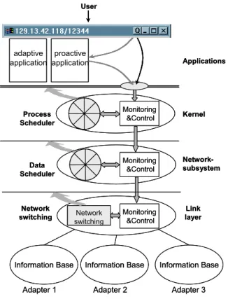
The overall picture of the QoS architecture is given in Figure 2.1. Basically, it consists of a set of Monitoring&Control entities, which are each associated with a resource. The resources currently under consideration in the end system are the processing time (processor scheduler entity), the available data rate shared between different flows and the available network links in a multi-homed end system. The Monitoring&Control entities monitor the resource sharing of the associated resource, i.e. they schedule the resource usage between the demands. The control part realizes the interaction with other Monitoring&Control entities. They accept demands for a modified resource share, and pass this demand down to another entity according to some adaptation and coordination rules. User Process Scheduler Data Scheduler Monitoring &Control Kernel Network-subsystem Applications proactive application adaptive application Information Base Monitoring &Control Monitoring &Control Network switching Network switching Link layer

Adapter 1 Adapter 2 Adapter 3

Information Base Information Base

User Process Scheduler Data Scheduler Monitoring &Control Kernel Network-subsystem Applications proactive application adaptive application Information Base Monitoring &Control Monitoring &Control Network switching Network switching Link layer

Adapter 1 Adapter 2 Adapter 3

Information Base Information Base

Figure 2.1: Overall Picture of our QoS Architecture

Many application-oriented approaches exist that try to maintain information about the application’s requirements and perform resource reservation in the end system based on ahead calculation of the need [3, 4]. Opposed to this, our QoS architecture is strictly user oriented. The resource sharing in the end system and the bias of the resource distribution should be done in favor of those applications the user is currently focusing on. This could be simply the window that is active in the moment, as it is done in the Windows 2000 operating system [5]. As this might fit

(8)

the user’s interest only some times, in [6] we proposed a simple user interface that allows the user to signal his current commitment to one or another application more explicitly. This interface is also shown in Figure 2.1: A button labeled with the letter Q (denoting Quality of Service) is integrated into the window title bar of each application started on the system. This Q-Button can be integrated into any windowing system (X-Window as well as Windows 2000) and does not necessarily depend on an application.

It is the job of the operating system (and, if supported, of the application itself) to determine the meaning of “better”. The user is not concerned with technical details and parameters detaching him or her from productive work. Instead, the mapping of a single user parameter, given just by a click on a button, must be mapped onto different system parameters like processing time, data rate, used network, cost factors etc. (cf. [7]).

Different parts of the architecture have been realized up to now: The adaptive data scheduler is described in [5], the network switching is part of the current work. Whereas application adaptation is a well-known concept in distributed multimedia systems [8], we first introduced the notion of proactive applications [2, d]. In contrast to adaptive1_applications_{that try to adapt to the} current situation but cannot actively control resources, proactive applications actively take effect on the sharing of resources in advance. Thus, beside user interaction by means of the Q-Button applications can interact with the system on their own.

There are some basic design decisions that result from the presented architecture and follow the goal not to design a completely new operating system kernel:

& Inside each Monitoring&Control entity, minor resource variations should be hidden from the neighbor entities. Thus, short-term and long-term variations are going to be decoupled and the system stability is increased.

& The Monitoring&Control entities accept and deal with simple resource requests that are passed over from other Monitoring&Control entities as well as from proactive applications. In general, these requests result in a bias of the resource distribution in favor of the flow or process related to the request. Obviously, resources are limited and can not be increased, but they should be given to the application that is currently in the user’s focus. Thus a paradigm shift from calculation and reservation in advance to adaptation to the situation is performed and complexity is being reduced.

& Especially the CPU scheduling is crucial for both the behavior and the performance of an operating system. Hence, modifications of the used algorithms should be done very carefully, existing applications relying on some properties should not be broken.

1_{In our context, adaptive applications have the same meaning as}_{reactive applications}_{as they react on dynamic} environments by adapting to the current availability of resources.

(9)

Following these goals, in the next chapter the existing CPU scheduler in the Linux operating system is described and analyzed in more detail. Afterwards, the concept of an adaptive scheduler is presented in chapter 4.

(10)

(11)

3 Background: Scheduling and Policy-based Networking

within the Linux Kernel

The basic idea for providing applications with the quality of service they need is to use an adaptive process scheduler combined with an adaptive networking subsystem, as described in the previous section. Before the implementation of the adaptive process scheduler is described in more detail, we give an introduction in the scheduling of tasks within the Linux kernel. This helps to understand the decisions we made for the implementation of our adaptive process scheduler. According to the previous chapters, the following general conditions were taken into account: & Existing (“legacy”) applications should be executable further on without any restrictions.

Additionally, those legacy applications should also take advantage of the QoS support. & The mechanisms for achieving quality of service should be simple and efficient.

& The user (or the application, respectively) must be involved in the closed loop in an active way, i.e., s/he must be able to affect the quality of service for each application.

& If possible, encroachments in the mechanisms of the operating system should be minimized as modifications may result in an inappreciable behavior of the system.

3.1 Scheduling in the Linux Operating System

Within the Linux Kernel, the mechanisms for scheduling the available CPU resources to the running processes are primarily optimized for high efficiency, fairness, throughput and low response times. However, quality of service aspects were not considered for the development of the scheduler. For a running application it is not possible to use any QoS mechanisms related to the scheduling of tasks as a specification of the user’s preferences is not provided.

In the following sections, the terms process scheduling, thread scheduling, and task scheduling will appear several times, particularly in the context of the question, to which kind of objects the CPU resources are scheduled. In order to avoid obscurity, we use the generic term scheduling for allotting the available computation time.

A detailed description of further components and the mechanisms of the Linux kernel are described in [9, 10].

3.1.1 Basics: The Architecture of Linux

In contrast to the current evolution of operating systems towards a micro-kernel architecture, the Linux kernel bases on a monolithic architecture. This basic design aspect also affects the

(12)

functioning of the process scheduler. In micro-kernel architectures, e.g., the Mach Kernel [11] or the Kernel of Microsoft Windows 2000 [5], the operating system’s kernel only provides a minimum of functionality for performing basic operations. Examples are the inter-process communication (IPC), and the memory management (MM). Built on top of the micro-kernel, the remaining functionality of the operating system is implemented in independent processes or threads running in the user space. They communicate with the micro-kernel via a defined interface. For the scheduling of the available computing time, the micro-kernel only supports the basic mechanism for switching from one process or thread to the next, called a context switch. The schedule sequence of the processes or tasks is determined separately, e.g., by kernel threads.

In monolithic architectures – like the Linux operating system – the entire functionality is concentrated within the kernel, i.e., all mechanisms and information relevant for the scheduling are available in the kernel.

CPU CPU User Mode System Mode Hardware Processes Tasks Scheduler

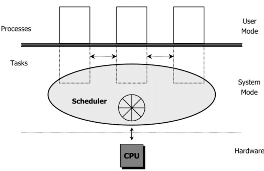
Figure 3.1: The Architecture of the Linux Operating System

Figure 3.1 gives a coarse view on the Linux architecture, focused on the interaction between applications, scheduler, and hardware. Further resource managers like the memory manager are not shown in Figure 3.1 as the illustration might become too complex. Like other operating systems such as Microsoft Windows 2000 [5], a Linux process resides in one of two modes; a privileged system mode, and a non-privileged user mode. In general, applications are running as processes within the user mode. Each process exists independent from other processes; i.e., each process has its own memory space and is not allowed to access the memory of other processes. When a process enters the Linux kernel (e.g., in the case of an interruption or a system call), the system switches to the privileged system mode. In the Linux operating system, only one process can be

(13)

executed in the system mode, as the kernel performs critical operations which must be protected from mutual preemption2_{. From the Linux kernel’s point of view, the processes are noted as}_tasks and are treated like common functions. In Figure 3.1, the tasks are marked by the dotted lines of each process resumed in the system kernel. Once a process/task enters the privileged system mode, it has access to the resources of every other task currently running on the system, which is not possible in the user mode. The scheduler is completely implemented inside the operating system’s kernel. In multi-processor environments, each processor has its own scheduler, but the scheduling algorithm used by each scheduler is always the same.

3.1.2 Processes, Threads and Tasks

In papers about Linux, the terms process, thread, and task are in many cases handled with the same importance, although they are completely different. A process is generally defined as a sequence of activities related to a distinguished “problem”. Each process exists independent of other processes. Processes are not able to affect each other, albeit they can communicate with each other using kernel mechanisms for inter-process communication. Thus, switching from one process to the next one requires a complete switch of the environment, including address space and CPU registers.

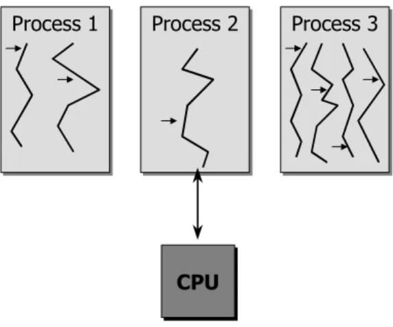
Within a process’ address space, one or more threads could exist in parallel working on the same “problem”. Those threads are running within the same environment, i.e., switching from one thread to the next only requires a fast context switch rather than an extensive switch of the environment. Thus, threads are also known as light-weighted processes. Another important differentiation is that parts of the process’ memory space (the so called shared memory) are accessible by all threads running within that process. This feature allows for an easy and efficient synchronization of threads and an efficient data exchange between threads as no communication paths have to be established. The basic difference between threads and processes is illustrated in Figure 3.2. (Note that Figure 3.2 is a typical example for a multi-threading operating system, such as Solaris. It is not typical for Linux!) Within the environment of a process, one or more threads are running simultaneously. The arrows mark the current position of the instruction counter for resuming the computation. In multi-threaded operating system designs, threads are dispatched immediately to the processor, whereas in Linux processes are scheduled and threads might run within a process as described below.

2_{Note that even in multi-processor environments only one process could be executed within the system} mode.

(14)

Process 1

Process 1 Process 2Process 2 Process 3Process 3

CPU CPU

Figure 3.2: Difference between Processes and Tasks

From the viewpoint of the Linux kernel, every process running on the system is referred to as a task. Compared to processes, tasks are allowed to access every resource (in particular, tasks are allowed to modify other tasks), as they are running in the privileged system mode. Thus, the scheduling algorithm running in the kernel shares the available CPU bandwidth between the tasks currently running on the system, independent whether a task represents a process or a thread outside the Linux kernel. The task’s structure is defined in include/linux/sched.h (see struct task_struct) and contains parameters that characterize a task, such as memory management information, various variables for states, flags, and statistics, pointers to related tasks (such as child tasks, parent tasks, previous and next task in the task-list, etc.), hash tables, process credentials, limits, file system info, signal handlers, etc. The definition of the complete task structure is printed in Chapter 0.

Originally, threads were not supported from the Linux operating system; applications were basically mapped to processes. In order to achieve compatibility to the POSIX 1003.1c standard [12] relevant for UNIX operating systems, there are two basic implementation designs enabling the use of threads in Linux. The basic difference between those approaches is the way how the scheduler treats threads:

& The first approach is the implementation of threads within a process, implemented by the PThread library [12]. If a process starts one or more PThreads, it is responsible for scheduling the computation time he gets from the operating system’s scheduler to the PThreads currently running within its context. Thus, PThreads are invisible for the scheduler as they are completely implemented within the user space.

& The alternative is the mapping of threads to processes, i.e., each thread is represented by exactly one process. One example for this approach is the system call clone() (defined in arch/i386/kernel/process.c) Using this system call, a new process is forked, that is allowed to access a shared memory allocated from the parent’s process. In this case, the

(15)

Linux scheduler is responsible for sharing the computation time between all threads, as those threads are represented as common tasks for the kernel. Thus, the more threads created by a process or an application, the more computation time is scheduled for this application. In the remainder of this document, the differentiation between processes, threads, and tasks is not considered as the scheduler of the Linux operating system is responsible for scheduling the available computation time to tasks. Note that the definition of the task structure (struct task_struct) can be found in include/linux/unistd.h.

3.1.3 Scheduling

The principle job of the scheduler is to decide the next executable task that is dispatched to the CPU. A task is marked as executable, if the computation of the task can be (actively) continued and does not depend on any other resources, such as arriving data from a hard disk drive. From the implementation point of view, a task p is executable if its actual state is p->state = TASK_RUNNING. The scheduling functionality can be found in kernel/sched.c in the function schedule(). In Linux, the scheduling works in a preemptive manner, i.e., a task will run as long as one of the following events occur:

& the task voluntarily releases its control back to the scheduler, or

& the scheduler revokes the CPU resource from the active task and dispatches the CPU to another task.

The scheduling sequence is defined by a round-robin-based time division multiplexing mechanism. Each (executable) task is dispatched to the CPU for a short period of time. This period, the so-called time slice, has a value of 200 ms in Linux (defined in the constant variable DEF_PRIORITY in include/linux/sched.h). For each task currently dispatched to a processor, the time slice will be counted downwards. If the time slice expires, the active task will be preempted in favor of another task. An expired task will not be dispatched until the time slice of each executable task is expired. After this time, all tasks – including the non-executable – will be re-initialized and the competition for the CPU starts from the beginning.

In Linux, time is measured in ticks (specified in kernel/timer.c) defined by the constant variable HZ in the file include/asm/param.h(for x86-based CPU architectures). The temporal resolution of time depends on the CPU architecture. In x86-based processor architectures, one tick corresponds to a time period of 10 ms (HZ = 100), whereas in the Alpha architecture, the time is updated 1,024 times per seconds3_{, i.e., one tick takes 0.977 ms. The time [in ticks] passed since the} last system startup is stored in the global variable jiffies, defined in the file

(16)

include/linux/sched.h. However, in many documents about the Linux kernel, ticks and jiffies are used in the same sense.

As mentioned above, the scheduler will be called in three cases: 1. The time slice of the active task expires.

2. A task voluntarily releases the control back to the scheduler (e.g., it has to wait for a resource).

3. An interrupt or a system call triggers the scheduler.

The functioning of the scheduler can be subdivided in three steps. First, interrupts that were not handled completely have to be finished. The second step is the selection of the next task that will be scheduled to the CPU. Finally, the new thread will be dispatched to the CPU. The three steps are explained in the following sections in more detail.

3.1.3.1 Interrupt Handling

Interrupts are used for notifying the operating system that certain events occurred, e.g., a completed data transfer or an error in a peripheral device. Interrupts are handled within the kernel of an operating system; therefore, the system switches to the privileged system mode. In Linux, three types of interrupts can be distinguished:

& Fast interrupts like the input of characters via the keyboard require no time-sensitive actions and are handled immediately. For the scheduler, the handling of fast interrupts is transparent; it can only be noticed by the system that there is less time available for the tasks.

& In contrast to fast interrupts, a slow interrupt could be intercepted by other interrupts. The handling of slow interrupts is realized in two steps. First, actions that are essential for handling the interrupt are performed. The remaining operations for its completion, called

bottom halfs, are carried out when the scheduler is called the next time. The completion of the interrupt routine is performed before the scheduling algorithm starts; on account of the 20 ticks for the initial time slice, the maximum amount of time for the completion is 200 ms. The system timer is a typical example for a slow interrupt, which is released every 10 ms by the processor (on x86-based architectures). The actions in the first step are generally to update the system time, i.e., by incrementing the jiffies. Later, the bottom half takes care on executing expired timers and updating statistics for the currently scheduled task.

(17)

& The third type of interrupt is a system call. A system call requires to enter the system mode, which is realized by a soft interrupt4_{. The scheduler is never called directly; instead, the} need_resched flag (defined in the task structure in include/linux/sched.h) of an executable task is set to 1. This flag is automatically checked after the completion of a system call and, when appropriate, the scheduler will be triggered.

If the scheduler is executed, the first step is to complete the bottom halfs. In the Linux 2.3.49 kernel, the existence of bottom halfs are indicated by the variable tq_scheduler, defined in include/linux/tqueue.h, as can be seen by the following lines of code.

444 if (tq_scheduler)

445 goto handle_tq_scheduler;

If the tq_scheduler flag is set, the function run_task_queue() (also defined and implemented in include/linux/tqueue.h) will be called which works out all bottom halfs that were marked by interrupt handling routines. Basically, the same procedure is performed in the next step for handling the “bottom halfs” of software interrupts.

457 if (softirq_state[this_cpu].active & softirq_state[this_cpu].mask) 458 goto handle_softirq;

The treatment of software interrupts is performed by the function do_softirq(), which is implemented in kernel/softirq.c and basically works in the same way as described in the previous case.

3.1.3.2 Scheduling Algorithm

The scheduling algorithm in Linux is responsible for deciding which (executable) task is next dispatched to the processor. According to the POSIX 1003.1b standard [13] for UNIX operating systems, Linux distinguishes two classes of tasks: real-time tasks and common tasks. Compared to common tasks, real-time tasks are principally favored by the scheduler. They only have to compete with other real-time tasks for the available computation time. For scheduling real-time tasks, the POSIX 1003.1b specification defines two operations: Periodic real-time tasks are scheduled by a round-robin-based algorithm, whereas a sporadic real-time task is executed until it voluntarily releases the control over the CPU or until a real-time task with a higher priority preempts it, whereas periodic real-time tasks are preempted by the expiration of their time slice. In the Linux kernel, the

4_{A soft interrupt is initiated by software. In Linux, soft interrupts for switching to the system mode are} realized by calling the interrupt 0x80.

(18)

different types of tasks are defined in include/linux/sched.h. Periodic real-time tasks are represented by SCHED_RR, sporadic real-time tasks by SCHED_FIFO, and common tasks by SCHED_OTHER.

Before the core scheduling algorithm starts, some actions need to be performed that guarantee a correct and fair scheduling of the available CPU resources. The active periodic real-time task is appended to the end of the queue of real-real-time tasks, so other “equal” real-real-time tasks will also be scheduled. Furthermore, tasks waiting for specific events must be marked as executable if the corresponding signals arrive [10]. Further modifications of a task’s state are described in [14]. However, those modifications are only relevant for scheduling in a way that the set (realized as a list) of executable tasks is updated.

For the decision of the next task that will be dispatched to the CPU, the scheduling algorithm computes a weight for each executable task. This task is implemented in the function goodness() (in kernel/sched.c) and will be described in more detail. As real-time tasks are favored, it seems that there are different schedulers for each kind of tasks. Indeed, both common tasks and real-time tasks are scheduled by the same scheduling function. Only the weight function differs for each class of tasks.

3.1.3.2.1 Real-Time Tasks

The priority of real-time tasks potentially running in the system is always higher compared to common tasks. Thus, a real-time task only has to compete with other real-time tasks for the available computation time. Therefore, a fixed priority scheme is used, where the decision for the next task dispatched to the CPU is exclusively determined by the real-time priority of a task, defined in the variable rt_priority (defined for each task). Other factors such as the current size of the consumed computation time are not taken into account. Generally, the task with the highest real-time priority will be executed; it has to share the CPU bandwidth with other real-real-time tasks having the same real-time priority. If a task with a lower priority currently runs on the system, it will be preempted. A dynamic modification of the real-time priorities is in general possible by external programs, however, the scheduler does not alter their values. Thus the weight calculated for each real-time task is constant (if one of those external programs does not modify the real-time priority). An expired time slice causes the preemption of a periodic real-time task, which will be re-initialized immediately.

The calculation of a real-time’s weight is very simple, as can be seen by the following two lines of code in the goodness() function:

120 if (p->policy != SCHED_OTHER) {

(19)

A real-time task that is not marked with the SCHED_OTHER flag gets a weight of its (constant) real-time priority plus 1,000. This weight could not be reached by any common tasks; thus, executable real-time tasks are always treated before any common tasks.

The handling of real-time tasks reveals that the term “real-time” is not appropriate in this context. Typically, a real-time task has to deliver a correct value within a pre-determined time. Although a Linux-based application can affect the real-time priority of its process, there is no correlation to the support of a guaranteed quality of service, as neither a reservation nor any admission control is performed. “Real-time” in the context of Linux only means that real-time tasks have a higher priority as common tasks. The scheduler handles real-time tasks according to the POSIX 1003.1b definitions [12]. Nevertheless, the term “real time” will be used further on in this paper as both the literature on Linux as well as the source code of the Linux kernel use this term. (Note that with RT-Linux [15] there is an extension to Linux supporting hard real-time capabilities!)

3.1.3.2.2 Common Tasks

Common tasks are only scheduled if no executable real-time task currently runs on the system. The scheduling mechanism uses a round-robin-based algorithm, where the scheduling sequence can change dynamically. In contrast to real-time tasks, other parameters are used for the calculation of a task’s weight. For common tasks, the weight function guarantees a fair scheduling, which is not necessarily given for real-time tasks. All parameters used by the weight function are defined for each task in the task’s structure (struct task_struct, see Appendix C).

& Time slice: The current size [in ticks] of the time slice. This value is defined in the variable counter and is decreased when the task is scheduled to the CPU. Thus, if a task’s time slice expires, counter is 0. The time slice is the basis for the weight function. If the time slice expires, the scheduler has to re-initialize the counter variable (which is done if the time slice of each executable task is expired).

& Processor switch: This parameter is only used if symmetric multi-processing is enabled. In SMP environments, each CPU has its own scheduler. Therefore, a slight advantage is given to the task’s weight if the task was last dispatched to this CPU, as the processor’s cache might still contain valid entries for the environment of this process and might not to reload the complete environment from memory. Additionally, some valid address mappings could have remained in the CPU’s TLB (translation look-aside buffer). This advantage gets lost when the task switches to another processor. The processor switch parameter is implemented by adding PROC_CHANGE_PENALTY to the weight. The schedule penalty is defined in include/asm/smp.h and is set to 15.

(20)

& Environment switch: Tasks running in the same memory as the current task (which could be realized by forking “threads” with the clone() system call, see section 3.1.2) are additionally preferred by increasing their weight. In this case a more efficient context switch (restoring the processor registers) is sufficient for switching to the next task instead of switching to a completely new environment. This slight advantage (which is implemented by incrementing the weight) results in an improved efficiency, albeit it contradicts to the principle of fairness for common tasks.

& Priority: In the Linux operating system, the priority has two meanings. First, it defines the (minimum) size used for the initialization of the time slices (in the counter variable) if all executable tasks are expired and need to be re-initialized. The priority is implemented in the task_struct’s variable priority and has a pre-defined value of 20 ticks for Intel architectures. That is why the default value for a time slice is 200 ms; it guarantees a fair sharing of the available computation time between the executable tasks. priority is not a static variable; e.g., the nice command (only available for root) manipulates the priority of a task, and thus its share on the CPU resources. The second meaning of the priority arises in its use for the weight function, as it is added to the parameters listed above. Therefore, processes with a lower priority are indirectly penalized as their time slice will not be consumed up as fast as the time slice of tasks with a higher priority. Note that the priority used for common tasks is different from the priority used for weighting real-time tasks (rt_priority), which is of no relevance for common tasks.

With the description of the parameters involved in the calculation of the weight for common tasks, the following lines of code which implement the core functionality of the goodness () function summarize those facts and are easy to understand:

132 weight = p->counter; 133 if (!weight)

134 goto out; 135

136 #ifdef __SMP__

137 /* Give a largish advantage to the same processor... */ 138 /* (this is equivalent to penalizing other processors) */ 139 if (p->processor == this_cpu)

140 weight += PROC_CHANGE_PENALTY; 141 #endif

142

143 /* .. and a slight advantage to the current MM */ 144 if (p->mm == this_mm || !p->mm)

145 weight += 1;

(21)

147 148 out:

149 return weight;

As can be seen in line 133, the weight will not be calculated for expired tasks (i.e., counter must be greater than 0). The basis is the currently remaining time slice (counter), maybe increased by the PROC_CHANGE_PENALTY if SMP is enabled in the kernel configuration (see above), maybe incremented if an environment switch can be avoided (line 145), and finally increased by the priority in line 146. Note that all the information used for the calculation of the weight function is stored in each task’s structure. The only sense of the goodness() function is basically to determine the next task that is dispatched to the CPU. It has no effects on the share a task gets on the available computation time – this share is defined only by the remaining time slice, represented in the counter parameter (as described above).

Compared to the calculation of a task’s weight, the scheduling algorithm works quite easy, as can be seen in the code printed below. The scheduling algorithm uses the goodness() functionality. However, it might be possible that the active task gives up its control voluntarily. This is marked by setting the task’s state to SCHED_YIELD. Thus, for the active task, the prev_goodness() routine will be called, which first checks if the SCHED_YIELD flag is set. In this case, the task becomes no weight (weight = 0), otherwise the weight will be computed according to the goodness() routine.

486 /*

487 * this is the scheduler proper: 488 */

489

490 repeat_schedule: 491 /*

492 * Default process to select.. 493 */ 494 next = idle_task(this_cpu); 495 c = -1000; 496 if (prev->state == TASK_RUNNING) 497 goto still_running; 498 499 still_running_back: 500 list_for_each(tmp, &runqueue_head) {

501 p = list_entry(tmp, struct task_struct, run_list); 502 if (can_schedule(p)) {

503 int weight = goodness(p, this_cpu, prev->active_mm); 504 if (weight > c)

(22)

506 }

Starting with the idle task (line 494; which is always on the first position in the run queue), for each (executable) task in the run queue it is checked whether the task could be scheduled or not (line 502). This check is only of relevance for SMP systems; in single CPU environments, the can_schedule() routine is always true. Therefore, for each executable task the goodness() function is called, whereby the helper variable c (line 495) stores the highest value of weight. This process shows that there is a second aspect that influences the determination of the next task – if two tasks have the same (highest) weight, the one that is positioned in front of the other tasks in the run queue wins the competition for the CPU resources. Remember that tasks with an expired time slice have a weight of zero. If the time slice of all executable tasks is expired, their time slices will be re-initialized, as described in the following section.

3.1.3.2.3 Initialization of Expired Tasks

If the time-slice of a periodic real-time task expires, the scheduler re-initializes its time slice immediately by assigning the value stored in the priority parameter, i.e., task->counter = task->priority, as can be seen in lines 624-629 (Appendix D). In contrast to real-time tasks, common tasks are only re-initialized if the time slice of each executable task is expired. In this case, all tasks will be re-initialized – including the tasks that are currently not executable. Thereby, the response time for tasks waiting for some resources is improved to achieve a faster reaction to the signal(s) the task is waiting for. The code for the re-calculation of the expired timers is also quite easy to understand. In order to avoid undefined states while modifying the task’s parameter, the task list (tasklist) has to be locked; other routines are allowed to read the parameters, but not to modify them (line 603). After the re-initialization, the run queue is unlocked (in line 607).

599 recalculate: 600 { 601 struct task_struct *p; 602 spin_unlock_irq(&runqueue_lock); 603 read_lock(&tasklist_lock); 604 for_each_task(p)

605 p->counter = (p->counter >> 1) + p->priority; 606 read_unlock(&tasklist_lock);

607 spin_lock_irq(&runqueue_lock); 608 }

(23)

The re-initialization of the time slices is done in line 605. Additionally to the priority parameter, the half of the original size of the remained time slice is added. Therefore, the new size of the time slice will be calculated according to the following equation:

»¼ » «¬ « + = 2 timeslice old priority timeslice new

This guarantees that tasks waiting for resources (and, thus, do not completely utilize their time slice) can react more spontaneous if the resource will become available. Dividing the time slice is realized as a simple and efficient bit shifting. Note that tasks with an expired time slice are re-initialized only by the priority (which is equal to 200 ms) as their counter is zero. If, as an example, a re-initialization is invoked and a (waiting) task has a remaining time slice of 17 ticks, it will be reinitialized with (20 + ¬17/2¼ ) ticks = 28 ticks. If the scheduler is called the next time, this task will be preferred as the time slice is the basis for calculating a task’s weight. Additionally, the CPU’s bandwidth will be shared more equally between the tasks as the computation time currently not needed will be particularly available later. Albeit the time slice for a waiting task seems to be increasing with every re-initialization, it has a maximum threshold of the double priority (i.e., 40 ticks), which can be easily proved by induction (see Appendix E for the proof).

In the case that no executable task currently exists, Linux provides a special task that is always executable. This task is called the idle task and is scheduled in this situation. The idle task is implemented as a simple endless loop, which is defined as a pre-processor macro in the file kernel/sched.c. Accordingly, the operating system provides an idle task for each CPU in SMP environments.

3.1.3.3 Dispatching

The task with the highest weight wins the competition for the resources of the CPU and has to be dispatched in the last step of the scheduling to the corresponding processor. Before this step is done, some statistical operations are performed. For the current task, the kstat.context_swtch variable (line 558) is incremented which stores the current number of preemptions. Additionally, in multi-processor environments, the average utilization of the time slice is computed (lines 535-548). For dispatching, the context (which are the register values of the processor) of the preceding task must be saved, before the new context could be loaded from memory. The components of a context are described in [16] in more detail, as architecture specific characteristics are taken into account. Note that the scheduler itself is not related to any task; until this point of time the scheduler runs in the context of the previous task that should be preempted. After dispatching, the scheduling is finished.

(24)

If the time slices of all executable tasks are expired, the time slices will be re-initialized (as described above) and the weight function for each executable task will be repeated. For dispatching the next task, the scheduler first switches the memory context (lines 568-586), before it loads the context of the new task in the CPU registers using the switch_to() function in line 592 (note that this routine is completely written in assembler code, see include/asm/system.h).

The following section gives a simple example of the scheduling.

3.1.4 Example

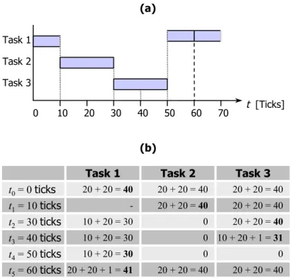
Figure 3.3 (a) demonstrates the scheduling in an example using three executable (common) tasks. At the time point t0 = 0 ticks, all tasks have a remaining time slice of 20 ticks (which means that they were just re-initialized) and the task running before t0 has to wait for any resource. We also assume a system running with one CPU.

Task 1 Task 2 Task 3 0 10 20 30 40 50 60 70 t [Ticks] (a) (b) t₀= 0 ticks 20 + 20 = 40 20 + 20 = 40 20 + 20 = 40 t1= 10 ticks t₃= 40 ticks t5= 60 ticks t2= 30 ticks t4= 50 ticks 10 + 20 = 30 10 + 20 = 30 0 20 + 20 = 40 0 0 Task 1 -10 + 20 = 30 20 + 20 + 1 = 41 Task 2 Task 3 20 + 20 = 40 20 + 20 = 40 0 10 + 20 + 1 = 31 20 + 20 = 40 20 + 20 = 40 Figure 3.3: Example for Scheduling of different Tasks

The dotted lines in Figure 3.3 mark the time points of the scheduler’s activation. While running, the weight will be calculated for each of the three tasks according to 3.1.3.2.2. Te results of the goodness() function are listed in Figure 3.3 (b), and base on the following calculations:

(25)

& t0 = 0 ticks. At the beginning of the example, no task has consumed anything of its time slice. Thus, the weight of 40 results by adding the time slice (counter, 20 ticks) to the priority (20 ticks). As Task 1 is the first in the run queue, it will be dispatched.

& t1 = 10 ticks. After 100 ms, Task 1 voluntarily gives the control over the CPU back to the scheduler as it has to wait for an external resource. At this point, the weight for Task 2 and Task 3 are still 40 as described above. Thus, Task 2 is the next task in the run queue and will be dispatched.

& t2 = 30 ticks. The time slice from Task 2 expires resulting in the activation of the scheduler. The weight function will weight Task 2 with 0 as its time slice has expired. Thus, Task 3 will be scheduled to the CPU.

& t3 = 40 ticks. Task 1 is signaled that the needed resource is now available and, the scheduler will be called. Thus, Task 1 becomes executable and will be weighted with 30 as its remaining time slice is 10 ticks. Task 3, which has also a remaining time slice of 10 ticks, will be kept dispatched, as it’s weight is 31 due to the advantage that no switching of the memory context is needed.

& t4 = 50 ticks. The weight for Task 2 and Task 3 is 0 as the time slices of both tasks are expired.

& t5 = 60 ticks. At this point, all time slices are expired and the scheduler initiates a re-initialization, which results in a weight of 0 for all tasks. Thus, the time slice of all tasks will be re-initialized and the weight will be computed a second time for each task. Note that after the re-initialization, Task 1 will keep the control over the CPU as no memory context switch is needed and, thus, the new weight will be 41 compared to 40 for Task 2 and Task 3.

This brief and simple example demonstrates the rather inflexible but efficient work of the scheduler. However, the support for quality of service is not possible as the Linux kernel does not support possibilities to affect the scheduling of the tasks. The following section describes the problems and the realization of an adaptive task scheduler for supporting quality of service to applications.

(26)

(27)

4 Design Issues for an Adaptive Scheduler

An adaptive scheduling mechanism is the basis for supporting quality of service on operating system’s level. Our approach is to realize an adaptive scheduler with a minimum of modifications at the fundamental scheduling mechanisms in Linux. Therefore, two basic possibilities can be identified: The use of periodic real-time tasks with dynamic priorities, or a flexible time slice scheme for common tasks. We decided to realize the second approach, as the use of dynamic real-time priorities has several disadvantages:

& A problem we identified in many tests is the favored treatment of real-time tasks. In general, an executable real-time task is always scheduled before all other common tasks and must not compete with them for the CPU resources. If a complex multimedia application bases on one or more real-time tasks, the performance of all other applications running on the system will break down.

& Dynamic real-time priorities require an extensive and complex priority management. A Real-time QoS Manager (RTQM) would be necessary to handle the scheduling policy of QoS-based applications. As an example, the RTQM has to perform a continuous adaptation of the real-time priorities for all tasks in order to guarantee the desired sharing, as the Linux scheduler only considers executable tasks with the highest real-time priority.

& The Real-time QoS Manager also has to handle the priority inversion problem, which occurs by the use of flexible priorities for real-time tasks. In the priority inversion problem, a low priority task that currently uses a resource blocks a (running) task with a higher real-time priority that tries to access this resource. Therefore, the RTQM has to perform additional operations for (real-time) priority inversion or the temporary increasing of (real-time) priority.

& The last aspect is the real-time priority itself, which has no relation to the scheduled CPU resources. Therefore, no statement about the effective quality of service support will be possible. Particularly, it will become very hard to map the application’s QoS requirements to real-time priorities.

4.1 Variable Time Slices

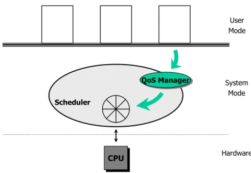
Instead of using dynamic priorities for real-time tasks for supporting quality of service on operating system’s level, we use a flexible time slice scheme for all tasks. Thereby, the component is of special interest that defines the priority of a (common) task and simultaneously defines the (minimum) time slice for its re-initialization. Thus, the basic idea of our approach is to use the priority variable as a representative for quality of service. As can be seen in Figure 4.1, we also

(28)

realized a QoS Manager that is responsible for interacting with the applications (see also chapter 2, note that QoS Manager and RTQM are different entities!). If a process requests an improved QoS support from the QoS Manager, it gets more CPU resources as its time slice will be increased. Note that the QoS Manager has to take into account whether scheduling more CPU resources to a task indeed improves the applications quality of service, or if the CPU resources are not the bottleneck. The mapping of different time slices to the corresponding amounts of CPU resources is implicitly performed by the scheduler. This approach additionally has the advantage that other tasks will not starve (which might be possible in the real-time approach), as the Linux scheduler will be called at the latest after all executable tasks are expired and, thus, were dispatched during this time period. Conversely, it has to be considered that the priority is at least one tick, as tasks with a priority of 0 are interpreted as expired and are not considered by the scheduler.

CPU CPU User Mode System Mode Hardware Scheduler QoS Manager QoS Manager

Figure 4.1: A QoS-based Scheduler for Linux

The QoS support specified by the user or an application can be easily mapped on the size of a task’s time slice. On account of the coarse resolution of time within the Linux kernel, we chose the identity function for the mapping. A modification of the quality of service support by “+1” results in an increase of the time slice by 1 tick. A formal description of the percental amendment on the share can be found in section 4.3.

Note that the mapping of the specified quality of service covers only the scheduled computation time. Predictions about the time points for the activation of the scheduler are not possible as this mainly depends on the unpredictable occurrence of interrupts and other system events. Thus, it is not possible to specify the triggering of the scheduler. It is only possible to determine the maximum time period between two calls of the scheduler, which is the double of the

(29)

maximum time slice (see section 3.1.3.2.3 and Appendix E). However, this also means that it is not possible to guarantee the desired quality of service to an application, as this basically depends on the behavior of the other tasks, interrupts and system events. That is, our approach only enables a statistical guarantee of the QoS support, which we call a soft quality of service. But, we believe that this kind of guarantee is sufficient for multimedia applications, as can be seen on the results described in [2].

Note that our approach described so far does not depend on explicit intervention in the scheduling mechanisms of the Linux kernel. However, there are some negative side effects, which require slight modifications of the scheduler.

4.1.1 Negative Side Effects

As some mechanisms of the Linux operating system are not designed for supporting quality of service within the end system, the use of variable time slices results in several negative side effects. As an example, the use of real-time tasks is in contrast to the QoS support, as those tasks are basically preferred and the user as well as the QoS Manager has rather any possibilities to control real-time tasks dynamically. One approach for avoiding this problem might be to treat real-time tasks as common tasks. In this case, only slight modifications of the scheduler are required. However, this encroachment contravenes against the POSIX 1003.1b specification [13], which explicitly postulates the existence of real-time tasks and their scheduling. Additionally, the modifications could result in an undesirable behavior of existing “real-time applications”. Thus, our approach treats real-time tasks as before. The user might remedy this disadvantage either by closing real-time applications, or (if s/he has root access) by using the system call sched_setscheduler(), which resets a real-time task to a common task.

A second obvious problem results from the demand-driven activation of the scheduler. A task that is currently dispatched to the CPU will only be preempted if it voluntarily releases the control over the CPU, if its time slice expires, or if a system call explicitly triggers the scheduler. Although this mechanism is very efficient for small time slices as the scheduler will only be called if it is necessary, it is disadvantageous for large time slices. If, e.g., two MPEG-2 videos are running with a time slice of one second, the CPU resources are shared equally between both applications. However, while running, the first application gets the complete CPU resources for 1 s and displays the video sequence with the maximum frame rate, while the other application is suspended. After 1 s, the time slice of the first video expires and the second video runs for 1 s, while the first applications is suspended. With a further increasing of the time slice, this effect is reinforced. However, this quality of service support is not in terms of the user’s satisfaction – it would be more convenient if both video sequences would be played simultaneously in a smoother way.

(30)

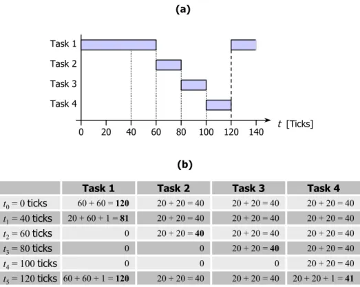
Another weak point that occurs from large time slices is the calculation of the weight for each task. The goodness() function uses the a task’s (re-)initialization value for the time slice (stored in the priority variable), resulting in a high weight for tasks with a large time slice. Thus, this task first utilizes its complete time slice, before other tasks are scheduled – even if the scheduler will be called multiple during this time period. This effect is clarified by the example shown in Figure 4.2. In this example, the time slice for Task 1 is 600 ms. Thus, its minimal weight will always exceed a value of 60 (until its time slice expires), which will never be reached by common tasks with a time slice of 20 ms. For common tasks, the maximum weight is 41 ticks (20 ticks remaining time slice + 20 ticks priority + 1 tick for avoiding a context switch). Note that the weights for each tasks at t5 in Figure 4.2 are the values for the second call of the function goodness(), after all tasks were re-initialized.

Task 2 Task 3 Task 4 0 20 40 60 80 100 120 140 Task 1 t [Ticks] (a) (b) t₀= 0 ticks 60 + 60 = 120 20 + 20 = 40 20 + 20 = 40 t₁= 40 ticks t₃= 80 ticks t₅= 120 ticks t₂= 60 ticks t4= 100 ticks 0 0 20 + 20 = 40 20 + 20 = 40 0 0 Task 1 20 + 60 + 1 = 81 0 60 + 60 + 1 = 120 Task 2 Task 3 20 + 20 = 40 20 + 20 = 40 0 20 + 20 = 40 20 + 20 = 40 20 + 20 = 40 20 + 20 = 40 20 + 20 = 40 20 + 20 = 40 Task 4 20 + 20 = 40 20 + 20 = 40 20 + 20 + 1 = 41 Figure 4.2: Example for Tasks with large Time Slices

In the context of large time slices, the re-initialization after the expiry of a task’s time slice is also crucial for the QoS support. The specification of quality of service on the level of the operating system has no direct correlation to the time slice of a task. Additionally, a re-initialized time slice also depends on the current time slice (see line 605) and, thus, results in an unpredictable quality of service support, if the task has to wait for any resources. If, e.g., an adaptive video application with a priority of 100 ticks has to wait for incoming data, its time slice increases up to 2 s. If the data is available, the application gets the complete CPU resources for 2 s. Thereupon,

(31)

the quality of service support is degraded suddenly after the next re-initialization and the share of the CPU resources is settled down at the desired level. Thus, the improved response time for waiting tasks in Linux also affects the QoS support in a negative way. Additionally, variations in the quality of service support are caused by applications that do not completely consume their scheduled computation time, resulting in a dynamic balance between user requirements, current load, behavior of applications, and interrupts from the hardware.

4.2 A QoS-based Scheduling Approach

The effects described in the previous section show the need for encroachments in the basic scheduling mechanisms of Linux. Thus, the quality of service support from the operating system is achieved by a combination of two basic concepts: First, adaptation is achieved by using a flexible time slice scheme, which is controlled by a feedback loop. Additionally, a modified QoS-based scheduler cares for an improved quality of service support.

The negative effects result mainly from tasks with large time slices running on the system. Thus, one obvious approach could be a restriction of the maximal size for the time slice. Additionally, it is conceivable to reduce the priority and thus the (re-)initialization value (which is at least 20 ticks) for each task. However, this approach is rather inflexible, because it is on the one hand difficult to specify an upper limit for the time slices of all applications. On the other hand, the default granularity of the system time is very coarse (1 tick = 10 ms). Subsiding the priority level for all tasks, the granularity for adjusting the QoS support becomes much coarser (cf. section 4.3).

The alternative we used for handling tasks with a large time slice is the additional use of a time-driven mechanism for triggering the scheduler. Therefore, an external timer calls the scheduler periodically. The activation of this timer is only necessary, if the user or an application requires a QoS support. If the user needs no further quality of service (or a QoS-based application is terminated), the timer will be deactivated if no other QoS-based applications are currently running on the Linux system, resulting in the original efficiency of the scheduling mechanism. Thus, the external timer takes care for a more regular (and thus a qualitative better) QoS support of the operating system, as large time slices will be split in several smaller units that are dispatched to the CPU resulting in an improved interleaving of the tasks. We implemented the external timer by using the add_timer(), del_timer(), mod_timer()system calls, which periodically trigger our scheduler with a frequency of 100 Hz.

However, the external timer does not remedy the general problem of the coarse temporal granularity. Of course, a resolution of 10 ms causes little effort for the management of the timing aspects and the scheduling of tasks, but for current and future applications, this granularity is not sufficient as the desired frequency of the scheduler calls cannot be adjusted exactly. Note that a

(32)

six-times super-scalar processor such as the Intel Pentium 4 CPU running at 1.5 GHz performs 15,000,000 CPU cycles in 10 ms and is, thus, able to calculate theoretically up to 90,000,000 operations in 1 tick [17]. This suggests the idea of modifying the timing basis for Linux. Although this can be easily achieved by decreasing the HZ constant (currently set to 100 (file include/asm/param.h) for x86-based CPU architectures), which results in a shorter period for one tick. However, every routine handling temporal aspects (such as the calculation of the time, routines for statistic calculations such as the average time slice, etc.) has to be modified in order to achieve a correct system behavior.

However, tasks with a large time slice are still treated in the same way. As can be seen in Figure 4.2, Task 1 gets the CPU within the first 600 ms, even if in the scheduler is called within this time period. Afterwards, it has to wait for 600 ms until all other tasks with a smaller time slice are expired. A more regular scheduling policy can only be achieved by modifying the scheduling algorithm. The reasons for the behavior of tasks with a large time slice can be mainly seen in the goodness() function, as both the priority and the remaining time slice of each task are the most relevant parameters for the calculation of the weight. In order to obtain the effectiveness of the scheduler, we decided not to modify the basic scheduling mechanisms but to adapt the goodness() function in the following way. (In contrast to earlier versions of the Linux kernel, we wrote a new function in parallel to goodness() called goodness_qos(), which is only used by the scheduling algorithm as there are other functions [such as reschedule_idle()] that use the values generated by goodness().)

& For each task, we additionally retain the number of schedules in the variable schedule_counter (stored in struct task_struct in include/linux/sched.h). If all executable tasks are expired and their time slices are re-initialized, the schedule_counter will also be reset to 1. Thus, the weight will be computed as follows: For the basis, we use the currently remaining time slice divided by the number of schedules (and rounded to the lower whole-numbered value). Where applicable, both the advantage for avoiding of a CPU penalty as well as the context switch benefit are added to this value as described in section 3.1.3.2. Note that we have to take care that the weight does not become 0 as in this case the task will not be scheduled further on.

& Compared to the original goodness() function, the priority parameter is not considered in the weight.

& Another modification is required for the re-initialization of the time slices. As the time slice of a non-executable task increases, the control of the quality of service support becomes more difficult (and might even result in a degraded QoS support). Thus, we only re-initialize a task with its priority, i.e., it is easier to map the quality of service to the size of the time slice and the QoS support becomes more transparent and calculable to the application.

(33)

The following lines of code show the important part of the implementation of the goodness_qos() function.

1 static inline int goodness_qos(struct task_struct * p,

2 int this_cpu, struct mm_struct *this_mm) 3 { 4 int weight = 0; 5 ... 23 if (!(p->counter)) 24 goto out; 25 26 27 if (p->schedule_counter >= p->counter) 28 {

29 // schedule_counter must not get higher as the counter value, 30 // otherwise the DIV will become 0! Beware that there is no 31 // schedule_counter overflow. schedule_counter must not become 32 // 0, as in this case the following code will not be called. 33 // Set weight to 1 for optimization :-)

34 35 p->schedule_counter = p->counter; 36 weight = 1; 37 } 38 else 39 {

40 weight = (int) p->counter/p->schedule_counter; 41 }

42

43 #ifdef __SMP__

44 /* Give a largish advantage to the same processor... */ 45 /* (this is equivalent to penalizing other processors) */ 46 if (p->processor == this_cpu)

47 weight += PROC_CHANGE_PENALTY; 48 #endif

49

50 /* .. and a slight advantage to the current MM */ 51 if (p->mm == this_mm || !p->mm) 52 weight += 1; 53 54 out: 55 return weight; 56 } 57 58 #endif //CONFIG_QOS_SCHED

(34)

On the basis of this calculation, tasks that are dispatched quite often between two re-initializations will become slightly handicapped. However, in combination with the external timer described above, the available CPU resources will be scheduled much smoother between running tasks, as can be seen in the example in the next section.

Within the function responsible for the scheduling of tasks (schedule() in file kernel/sched.c), we only have to modify minor functionality. The first modification is to increase the number of schedules (p->schedule_counter) for the current task every time the scheduler is called. Second, we have to call the goodness_qos() function instead of the goodness() function for the calculation of each task’s weight. The third modification of the scheduler has to be done in the re-initialization of each task. We only use the priority value for the re-initialization and omit the current size of the time slice. Additionally, the schedule_counter parameter must be reset. Thus, the following lines of code perform the re-initialization of each task that currently exists on the Linux system.

1 for_each_task(p) 2 {

3 p->counter = p->priority; 4 p->schedule_counter = 1; 5 }

As can be seen in the previous lines of code, the effort of our adaptive scheduling mechanism only minimally increases the system load. Compared to the original scheduling mechanism, the adaptive scheduler needs an additional if-then-else construct in the goodness() function, which results in either two assignments of values to variables or a whole-numbered division of the variable weight (unfortunately, divisions are quite expensive in terms of CPU cycles). In return, we can omit one assignment and the addition of the priority to the weight. The scheduler needs an additional incrementing of the schedule_counter variable; the re-initialization also requires an additional assignment for the same variable, which is yet compensated by resigning on the calculation of the increased time slice if a task does not completely utilize its time slice (cf. line 605 in Appendix D). Altogether, we have an additional overhead of one if-then-else query with an eventual division when passing through our adaptive scheduler for the Linux operating system.

4.2.1 Example

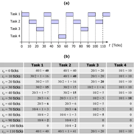
In order to demonstrate the behavior of our QoS-based scheduler, we used four tasks with different priorities. Task 1 and Task 2 have both a time slice of 40 ticks, Task 3 was initialized with

(35)

20 ticks and Task 4 had a pre-defined time slice of 10 ms. The frequency of the external timer was adjusted to 10 Hz, i.e., the scheduler was called every 100 ms. Figure 4.3 (a) shows the schedule sequence of the four tasks; in Figure 4.3 (b) the weights for the different tasks at each call of the scheduler can be seen. In the terms a/b in Figure 4.3 (b), a is the remaining time slice of the corresponding task at time ti, b represents the number of schedules (since the last re-initialization process) we introduced for our QoS-based scheduler, and the operator “/” denotes the division that rounds the result to the lower whole-numbered value. The bonus for avoiding a context switch was set to the default value of 1. The benefit for avoiding a processor switch is not

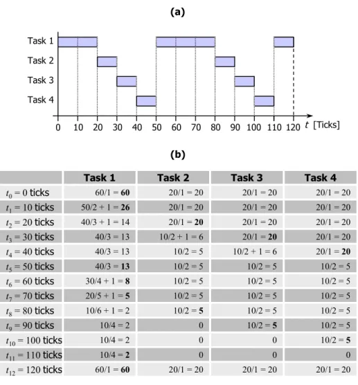
considered in this scenario (as we developed and optimized our adaptive scheduler for single-processor systems). In Figure 4.4, we demonstrate the schedule sequence with the same example shown in Figure 4.2. Task 2 Task 3 Task 4 0 20 40 60 80 100 110 Task 1 t [Ticks] 10 30 50 70 90 (a) (b) t₀= 0 ticks 40/1 = 40 40/1 = 40 20/1 = 20 t₁= 10 ticks t₃= 30 ticks t₅= 50 ticks t₂= 20 ticks t₄= 40 ticks 30/2 = 15 20/3 + 1 = 7 20/1 = 20 30/2 + 1 = 16 30/2 = 15 10/2 = 5 Task 1 30/2 + 1 = 16 30/2 = 15 20/3 = 6 Task 2 Task 3 40/1 = 40 20/1 = 20 30/2 = 15 10/1 = 10 20/3 + 1 = 7 10/2 = 5 10/1 = 10 10/1 = 10 10/1 = 10 Task 4 10/1 = 10 10/2 + 1 = 6 10/1 = 10 t₇= 70 ticks t₆= 60 ticks 20/3 = 6 20/3 = 6 10/2 = 5 10/4 + 1 = 3 20/3 = 6 10/2 = 5 0 0 t₉= 90 ticks t₈= 80 ticks 10/4 = 2 10/4 + 1 = 3 10/2 = 5 10/4 =2 10/4 = 2 0 0 0 t₁₁= 110 ticks t₁₀= 100 ticks 0 10/4 = 2 0 40/1 = 40 40/1 + 1 = 41 20/1 = 20 0 10/1 = 10

(36)

Task 2 Task 3 Task 4 0 20 40 60 80 100 110 Task 1 t [Ticks] 10 30 50 70 90 (a) (b) t0= 0 ticks 60/1 = 60 20/1 = 20 20/1 = 20 t1= 10 ticks t3= 30 ticks t5= 50 ticks t2= 20 ticks t4= 40 ticks 40/3 + 1 = 14 10/2 = 5 Task 1 50/2 + 1 = 26 40/3 = 13 Task 2 Task 3 20/1 = 20 20/1 = 20 10/2 + 1 = 6 20/1 = 20 Task 4 20/1 = 20 t7= 70 ticks t6= 60 ticks 30/4 + 1 = 8 20/5 + 1 = 5 t9= 90 ticks t8= 80 ticks 10/6 + 1 = 2 10/4 = 2 0 t11= 110 ticks t10= 100 ticks 10/4 = 2 0 0 20/1 = 20 20/1 = 20 20/1 = 20 20/1 = 20 20/1 = 20 40/3 = 13 10/2 + 1 = 6 20/1 = 20 40/3 = 13 10/2 = 5 10/2 = 5 10/2 = 5 10/2 = 5 10/2 = 5 10/2 = 5 10/2 = 5 10/2 = 5 10/2 = 5 10/2 = 5 10/2 = 5 10/2 = 5 10/2 = 5 10/2 = 5 10/2 = 5 0 0 0 10/4 =2 t12= 120 ticks 60/1 = 60 20/1 = 20 20/1 = 20 20/1 = 20 120

Figure 4.4: QoS-based Scheduling in the Scenario of Figure 4.2

As can be seen on the two examples, our QoS-based scheduler provides an improved quality of service support for the applications running on the operating system, as the scheduler is called more often and the QoS-based scheduling mechanism cares for a smoother schedule of the running tasks.

4.3 QoS Support in Theory and Practice

In our approach, the QoS support relates to the percentage of scheduled CPU resources within a time period. In this context, the time period is the time between two re-initialization processes. Assume that there are n executable tasks. Ti denotes the priority and, thus, the initial time slice for task i. If all tasks are executable, no further tasks are started and the CPU is completely utilized, the percentage share Ai on the available CPU bandwidth for task i is defined by the following equation.

(37)

¦

₌ = _n j j i i T T A 1

If the user (or an application) changes the priority for task Ti by ∆Ti [ticks], the percentage of he scheduled CPU resources ∆Ai for this task is defined by

¦ ¦

¦

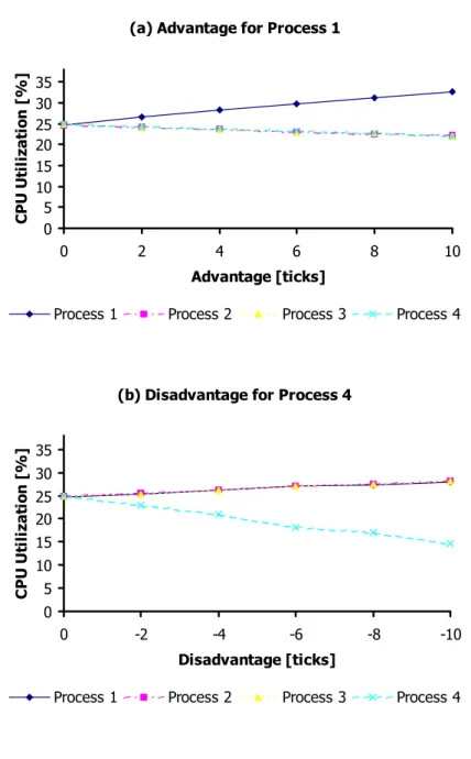
The derivation of this equation can be found in Appendix F. We also measured the system behavior in practice. Therefore, we started four processes performing integer additions in an endless loop and, thus, completely utilize their scheduled CPU resources, i.e., each process gets about ¼ of the available CPU resources while each process traced the time it was scheduled to the CPU. Figure 4.5 shows the results of this experiment. In Figure (a), we increased the time slice of process 1 by 2 ticks in each step, in Figure (b) process 4 was decreased by 2 ticks in each step. The two figures show the effect on the CPU utilization for each process. As we can see (which was already mentioned above), increasing the time slice for one task results in a lower increasing of the percentage on the CPU resources compared to a decreasing of the time slice5_{. Those experiments} show the feasibility of our adaptive scheduler. Further measurements, such as the result of the quality of service support for applications are described in [1, 2] in more detail. We also implemented a QoS Library that allows applications to specify their own quality of service support in order to achieve an optimized convergence of the QoS requirements to the actual QoS support provided by the operating system. A brief description of the QoS Library can be found in [2].

5_{Assuming the situation in Figure 4.5 starting with 20 ticks per process, increasing the time slice of Process 1} in (a) to 22 ticks results in an improved percentage of 1.829 %, whereas decreasing the priority of Process 4 (in (b)) results in a degraded percentage of 1.92 %.

(38)

(b) Disadvantage for Process 4 0 5 10 15 20 25 30 35 0 -2 -4 -6 -8 -10 Disadvantage [ticks] C P U U til iz at io n [ % ]