q1997 American Meteorological Society
What Controls Stratocumulus Radiative Properties?
Lagrangian Observations of Cloud Evolution
ROBERTPINCUS*ANDMARCIAB. BAKER
Geophysics Program, University of Washington, Seattle, Washington CHRISTOPHERS. BRETHERTON
Department of Atmospheric Sciences, University of Washington, Seattle, Washington (Manuscript received 13 May 1996, in final form 6 March 1997)
ABSTRACT
Marine stratocumulus clouds have a large impact on the earth’s radiation budget. Their optical properties vary on two distinct timescales, one associated with the diurnal cycle of solar insolation and another with the downstream transition to trade cumulus. Hypotheses regarding the control of cloud radiative properties fall broadly into two groups: those focused on the effects of precipitation, and those concerned with the environment in which the clouds evolve. Reconciling model results and observations in an effort to develop parameterizations of cloud optical properties is difficult because marine boundary layer clouds are not in equilibrium with their local environment.
The authors describe a new technique for the observation of boundary layer cloud evolution in a moving or Lagrangian frame of reference. Blending satellite imagery and gridded environmental information, the method provides a time series of the environmental conditions to which the boundary layer is subject and the properties of clouds as they respond to external forcings. The technique is combined with in situ observations of precipitation off the coast of California and compared with the downstream evolution of cloud fraction in five cases that were observed to be precipitating with three cases that were not. In this small dataset cloud fraction remains almost uniformly high, and there is no relationship between the presence of precipitation and the evolution of cloud fraction on 1- and 2-day timescales.
Analysis of a large number of examples shows that clouds in this region have a typical pattern of diurnal evolution such that clouds that are optically thicker than about 10 during the morning are unlikely to break up over the course of the day but will instead show a large diurnal cycle in optical depth. Morning cloud optical thickness and the resultant susceptibility to breakup have a much larger impact on diurnally averaged cloud radiative forcing than do diurnal variations in cloud properties. Cloud response is significantly correlated with lower tropospheric temperature stratification at all times, though the best correlation exists when cloud response lags stability by at least 16 h. Sea surface temperature is also correlated with cloud properties during the period in which cloud response is measured and the 12 h prior. The authors suggest that sea surface temperature plays two competing roles in determining boundary layer cloudiness, with rapid changes in SST promoting cloudiness on short timescales but tending to lead to a more rapid transition to the trade cumulus regime.
1. Introduction
Stratocumulus clouds in the subtropical marine boundary layer have a considerable impact on the earth’s radiative balance, primarily through enhanced reflection of incoming solar radiation relative to the underlying ocean surface. For a given area this impact is determined by both the reflectivity of the clouds present (which is
* Current affiliation: Climate and Radiation Branch, NASA/God-dard Space Flight Center, Greenbelt, Maryland.
Corresponding author address: Robert Pincus, Climate and Ra-diation Branch, Code 913, NASA/Goddard Space Flight Center, Greenbelt, MD 20771.
E-mail: [email protected]
in turn governed by cloud optical depth) and the amount of the area the clouds occupy (the cloud fraction). Ef-forts to elucidate the mechanisms controlling cloud frac-tion have been more common in part because cloud fraction, unlike optical depth, has been recorded by sur-face observers for many years and in part because cli-mate models have only recently begun to predict cloud optical depth by including budgets for cloud water. Knowledge of both quantities, however, is required to accurately model the effects of clouds on the surface and top-of-atmosphere radiation budgets.
Boundary layer cloud radiative properties vary on two distinct time and spatial scales. Cloud properties un-dergo considerable changes on hourly to daily time-scales that are driven by the diurnal cycle of solar in-solation. This diurnal cycle is superimposed on a more
gradual transition from the stratocumulus regime (with high fractional cloudiness and optical depth) to the trade cumulus regime. The transition occurs over thousands of kilometers, so that individual air columns experience the transition over about a week.
Hypotheses regarding control of boundary layer cloud fraction across the stratocumulus-to-cumulus transition fall into two broad categories. One set focuses on cloud microphysical processes, which are thought to act on cloud fraction through the production of precipitation in the form of drizzle. Precipitation may affect cloud fraction in two ways: by directly removing water from the boundary layer as drizzle at the surface and by mois-tening and cooling the layer below the cloud as falling drops evaporate. The second effect can inhibit the trans-port of warm, moisture-laden parcels from the ocean surface to the cloud and may promote a situation known as decoupling (Nicholls 1984). The link between cloud fraction and drizzle is quite strong in Albrecht’s (1989) diurnally averaged model of the marine boundary layer: in a two-dimensional version used to simulate subtrop-ical stratocumulus clouds off the coast of California, the elimination of drizzle increased cloud fraction by about 34% (Wang et al. 1993). This predicted sensitivity has not been confirmed by the observational record, how-ever. Austin et al. (1995), for example, discussed aircraft observations of drizzling stratocumulus during 3 days off the coast of California, while satellite imagery showed the cloud decks to be solid and continuous for hundreds of kilometers around the aircraft flight tracks. Austin et al. attributed the persistence of high cloud fraction to vigorous vertical transport of moisture from the ocean surface into the cloud layer by small eddies. A second line of inquiry centers on the role of the environment in determining boundary layer cloud frac-tion. Interannual variations of cloud fraction are cor-related with sea surface temperature (Norris and Leovy 1994; Klein et al. 1995) and with the amount of tem-perature stratification in the lower troposphere (Klein and Hartmann 1993), which is thought to be inversely related to boundary layer depth. Recent theoretical ev-idence (Wyant and Bretherton 1992) indicates that creases in boundary layer depth may be caused by in-creases in sea surface temperature, which lead to larger buoyancy fluxes and increased entrainment. Aircraft measurements (compare, e.g., Austin et al. 1995 and Martin et al. 1995) and numerical models (Bougeault 1985; Krueger et al. 1995; Wyant et al. 1997) show that the boundary layer tends to become more decoupled as its depth increases, while ship- and satellite-based ob-servations indicate that deeper boundary layers exhibit lower average values and larger diurnal variations of cloud fraction (Rozendaal et al. 1995). These obser-vations suggest a conceptual model that attributes the stratocumulus to trade cumulus transition to decoupling induced by downstream increases in boundary layer depth and associated increases in surface buoyancy and latent heat fluxes (Bretherton and Wyant 1997).
A strong diurnal cycle in cloud radiative properties is evident everywhere along the stratocumulus to cu-mulus transition path. The longwave radiative cooling that drives turbulent convection in the boundary layer occurs in the top few tens of meters nearest cloud top, but heating due to the absorption of solar radiation oc-curs at greater depths (Nicholls 1984). This distribution acts to destabilize the cloud layer and cause continued entrainment even as the cloud layer warms slightly and becomes decoupled from the air closest to the surface. Cloud base rises and cloud thickness decreases (Bou-geault 1985; Betts 1990; Hignett 1991) since entrain-ment drying is no longer balanced by fluxes of water from the surface. If the clouds are thin enough, cloud fraction may decrease as well (Rozendaal et al. 1995). Stratocumulus clouds in the marine boundary layer are influenced not only by the instantaneous environ-ment to which they are subject but also by conditions experienced during the past. Given the rapid variation in solar insolation over the course of the day it is un-surprising that clouds are thicker and more likely to decouple under a diurnal cycle than under average ra-diative conditions (Bougeault 1985). More remarkable is the effect of upstream conditions on cloud evolution across the stratocumulus to cumulus transition. Klein et al. (1995) found that changes in monthly mean cloud amount at a location in the northeast Pacific were better correlated with sea surface temperatures 24–30 h up-stream than with the local sea surface temperature, im-plying that boundary layer cloudiness adjusts to sea sur-face temperature on a timescale of at least a day. Bound-ary layer ‘‘memory’’ is also clear in theoretical studies: results from models run with temporally variable boundary conditions (Krueger et al. 1995; Wyant et al. 1997; Bretherton and Wyant 1997) or those that incor-porate advection terms (Wang et al. 1993) consistently differ from those run with fixed boundary conditions. Boundary layer depth in particular equilibrates to en-vironmental changes only on timescales of several days (Schubert et al. 1979). This suggests that the marine boundary layer is best observed and modeled in a La-grangian frame of reference following the average mo-tion of a column of boundary layer air.
A Lagrangian framework is attractive because bud-gets may be formulated without the use of hard-to-mea-sure advective terms. Such an approach is most appro-priate when the structure of the boundary layer is in-fluenced more by vertical than horizontal mixing (Breth-erton and Pincus 1995). Several simulations of the stratocumulus to cumulus transition have been made using Lagrangian (time varying) boundary conditions (Krueger et al. 1995; Wyant et al. 1997), but in situ Lagrangian observations are difficult to perform with traditional cloud physics obser vational platforms: ground- or ship-based remote sensing platforms can move slowly if at all, while instrumented aircraft have flight durations much shorter than the timescales over which cloud evolution occurs. Two in situ Lagrangian
FIG. 1. The Lagrangian observational technique. Operational en-vironmental analyses provide spatially and temporally varying wind, temperature, and moisture fields. Parcel trajectories and the history of the environment along them are computed from the wind fields. At regular intervals, visible and infrared images centered on the in-stantaneous parcel position are extracted from the large-scale images obtained by geostationary satellites. Each image in the time series is analyzed to determine cloud properties such as cloud fraction, cloud optical thickness, and boundary layer depth.
experiments (Bretherton and Pincus 1995) performed during the Atlantic Stratocumulus Transition Experi-ment (Albrecht et al. 1995) highlighted both the ad-vantages of this observing strategy and the many dif-ficulties that can arise in its implementation.
In this paper we use observations of the Lagrangian evolution of marine stratocumulus to examine the im-portance of precipitation and environmental evolution in the control of subtropical marine boundary layer cloudiness over the eastern Pacific. In section 2 we de-scribe a new technique for making Lagrangian obser-vations of cloud evolution from space and use the meth-od in section 3 to explore the role of precipitation in controlling cloud fraction. In section 4 we identify com-mon patterns of diurnal variability in cloud optical prop-erties, consider the radiative impact of these variations, and identify links between cloud response and the en-vironment in which the clouds evolve. We discuss the implications of our results in section 5.
2. Observing cloud evolution in a Lagrangian frame of reference
Our technique for observing the Lagrangian evolution of clouds from space is sketched in Fig. 1. The method uses a combination of operational weather analyses and imagery from operational satellites. Temporally and spa-tially varying winds from the synoptic analyses are used
to compute the trajectories of boundary layer air parcels as they are advected by the mean wind from their initial positions. At regular time intervals, mesoscale-size regions centered on the parcel position are extracted from the satellite image and cloud characteristics are estimated from the image. This process provides a time history of cloud properties and environmental condi-tions along the parcel trajectory.
a. Required datasets
The Lagrangian technique employs satellite imagery and gridded environmental information covering the geographical region and time period of interest. For studies of marine boundary layer evolution, we utilize visible and infrared wavelength images obtained at reg-ular time intervals, as well as gridded estimates of at-mospheric state and sea surface temperature. Investi-gations focusing on other portions of the atmosphere might well employ a different suite of data sources.
To achieve continuous temporal coverage in nonpolar regions we use visible (nominal central wavelength about 0.65mm) and infrared (11mm, in the water vapor window) images obtained from geostationary satellites. Infrared instrument counts are converted to brightness temperatures, while visible wavelength instrument brightness levels are mapped to values of directional reflectance (radiance normalized by the amount of in-cident radiation). Profiles of wind speed and direction, temperature, and humidity at all levels below 700 mb are taken from gridded global operational analyses. Sea surface temperature (SST) fields may be available as part of the operational analyses or as gridded fields based on satellite observations in the infrared.
Sections 3 and 4 describe studies of marine strato-cumulus off the coast of California. In those investi-gations we use atmospheric analyses supplied by the National Meteorological Center (NMC, now the Na-tional Centers for Environmental Prediction) on a 2.5-degree grid every 12 h at 1000, 850, and 700 mb. Sea surface temperature fields on weekly, 18-km grids are provided by the multi-channel sea surface temperature algorithm (MCSST; see McClain et al. 1985), which estimates SST from cloud-free infrared radiance obser-vations made by the AVHRR sensor aboard the National Oceanic and Atmospheric Administration (NOAA) po-lar-orbiting satellites. Satellite imagery extending north-east from 238N, 1358W is obtained from the VAS sensor from the Geostationary Operational Environmental Sat-ellite station at 1358W, which was occupied by the GOES-6 platform during the First ISCCP (International Satellite Cloud Climatology Program) Regional Exper-iment (FIRE) period. The images are produced every 30 min and have a nominal resolution of 1 km in the visible imagery and 43 8 km in the infrared imagery. Measurements at 6.7 mm replace the 11-mm imagery four times a day (at 0515, 1115, 1715, and 2315 UTC).
b. Determining parcel trajectories and the evolution along them
To compute an air parcel trajectory, we choose an initial position and starting time, then integrate the two-dimensional equations of motion on the spherical earth’s surface. At regular time intervals we report the parcel position and the interpolated values of the environmen-tal parameters (sea surface temperature, average wind speed, and vertical profiles of temperature and humidity) at that position. In our studies of boundary layer clouds we ignore vertical motion and vertical wind shear and use the wind fields at 1000 mb to determine the trajec-tory of boundary layer parcels.
Once a parcel trajectory has been computed, we ex-tract from the large-scale visible and infrared satellite images a mesoscale-size region (in the following stud-ies, 256 km on a side) centered on the parcel position at each reporting time. From this time series of images we use well-established techniques to estimate cloud properties (cloud fraction cf, cloud optical deptht, and
boundary layer depth zi) as function of time.
Cloud detection is necessary to determine cloud frac-tion, the ratio of the cloudy area in a scene to the total area, and is also a precursor to the determination of cloud properties, since these properties are defined for only those segments of an image that contain cloud. We choose two simple, independent, threshold-based cloud detection algorithms modeled on the ISCCP scheme (Rossow and Garder 1993). A pixel is labelled as cloudy if it is brighter (R.R01 DR in the visible wavelength
image, denoted VIS cloud fraction) or colder (T, T0
2 DT in the infrared image, referred to as IR cloud fraction) than the underlying ocean. For boundary layer clouds over the ocean the problem of determining clear-sky radiance is relatively straightforward, since both ocean albedo and surface temperature are fairly well constrained. We ascertain a regional average clear-sky reflectance by finding the average of the minimum value of reflectance at each pixel in the study region during the time period under consideration. The value of SST at the center of the image (interpolated from the SST fields) is assumed to accurately represent the ocean tem-perature. Threshold values are typically set to DR 5 0.03 (the relative uncertainty in visible wavelength cal-ibration; see Han et al. 1994) andDT53 K (the average of the temperature thresholds used in the ISCCP algo-rithm over coastal waters and the open ocean; see Ros-sow and Garder 1993). With such small threshold values pixels containing even a small amount of cloud are like-ly to be classified as fullike-ly cloudy. We use the two es-timates of cloud fraction independently; that is, we do not ensure agreement between the IR and VIS classi-fications on a pixel-by-pixel basis. The VIS classifica-tion is used to indicate valid pixels for the optical depth retrieval.
We estimate optical depth using a look-up table al-gorithm (Pincus et al. 1995) similar to the technique
used by ISCCP (Rossow et al. 1991) and other inves-tigators (Minnis et al. 1992). The algorithm compares the predictions made by a radiative transfer model of outgoing radiance as a function of cloud optical depth with observations of the radiance made by satellites and chooses an optical depth that minimizes the difference between the observed and computed reflectances.
We adopt the technique of Minnis et al. (1992) for inferring boundary layer depth (assumed to be equiv-alent to cloud top height) from estimates of SST and cloud-top temperature. Boundary layer depth zi(km) is
computed by dividing the difference between cloud-top temperature TC and sea surface temperature SST by a
temperature lapse rate of 7.1 K km21. We determine T C
by finding the median brightness temperature of those pixels classified as cloudy by the IR cloud detection algorithm and interpolate SST in space and time from the environmental fields.
c. Uncertainties in trajectory and cloud parameters Uncertainty in cloud and environmental properties de-rived along trajectories using the Lagrangian technique arises from three sources: uncertainty in the computed parcel trajectory, errors in gridded estimates of envi-ronmental parameters other than wind fields, and un-certainty in the measurement of cloud parameters.
1) SPATIAL TRAJECTORY
The Lagrangian observational technique has at its heart the parcel trajectories computed from the opera-tional analyses. Uncertainty in calculated parcel trajec-tories stems from uncertainties in the wind velocity fields provided by the operational analyses and inter-polated in space and time. Two questions arise: to what extent are the 1000-mb winds representative of the boundary layer winds, and how accurately do the anal-yses depict the true 1000-mb winds?
Winds at 1000 mb cease to represent the mass-weight-ed boundary layer wind velocity in the presence of ver-tical shear in either wind speed or direction. Although the amount of wind shear in the subtropical marine boundary layer varies in time and space, observations made off the coast of California from aircraft (Austin et al. 1995; Brost et al. 1982) and tethered balloons (Hignett 1991) consistently show little evidence of shear, suggesting that 1000-mb winds are sufficient for computing boundary layer trajectories. The accuracy of the analyzed wind fields is a thornier question. Over the ocean, the analyzed fields are synthesized from sparse ship and buoy reports and from cloud track winds, which are derived by following cloud features observed by satellites. A quantitative estimate of the uncertainty in the wind fields is difficult to determine, however, be-cause there are no independent estimates of wind speed and direction in the FIRE region to compare to the NMC analyses.
FIG. 2. Comparison of (a) temperature and (b) humidity at 850 mb as measured by radiosondes and as interpolated from gridded oper-ational analyses. The soundings were taken at San Nicholas Island near the coast of California during FIRE but were not included in the analyses. In this instance, the analyses are accurate with respect to temperature but are unreliable with respect to water vapor. Uncertainty in the analyzed wind fields leads to
uncertainty in the computed parcel trajectories. Kahl and Samson (1986) examined the uncertainty of tra-jectory calculations made over the central and eastern United States. They determined that winds interpo-lated from National Weather Service analyses in this region had randomly distributed errors of 2– 4 m s21,
which yields an uncertainty in position of about 200 km after 24 h and about 250 km after 36 h. Over the subtropical oceans the situation is somewhat more complicated: summertime winds are quite steady and easy to predict, but the measurement network is ex-tremely sparse. It is therefore likely that systematic (rather than random) errors dominate the uncertainty in computed trajectories. We have performed several sensitivity studies to assess this uncertainty, in which we perturb the analyzed wind fields by a fixed amount (10%–20% of the reported value, or biases of 1–2 m s21in each wind component) and recompute the parcel
trajectories. Although differences in final parcel po-sition can be large when long trajectories are consid-ered, we have found that differences in cloud evo-lution between pairs of original and perturbed trajec-tories are usually small compared to the differences among trajectories in a population.
2) TEMPERATURE AND HUMIDITY
The NMC analyses also provide a history of tem-perature and humidity throughout the atmospheric column along the trajectory. In contrast to the wind fields, independent measurements of these quantities were made during FIRE by approximately 70 radio-sondes launched from San Nicholas Island during FIRE by the Colorado State University CLASS sys-tem (Schubert et al. 1987). These soundings were not incorporated into the NMC operational analyses. The comparison is an optimistic one, since San Nicholas Island is quite close to the California coast and errors in lower tropospheric temperature and humidity are likely to increase with distance away from the land based sounding network.
Figure 2 shows a comparison between 850-mb tem-perature and water mixing ratio as measured during the radiosonde soundings and as interpolated from the NMC analyses. We compute the average temperature and wa-ter vapor mixing ratio from the soundings in the 10-mb layer around 850 mb and compare these values to the NMC analyses interpolated to the location of San Nich-olas Island at the time of the radiosonde launch. The figure suggests that in this location lower tropospheric temperature estimates from NMC analyses are quite rea-sonable but that moisture estimates show too little vari-ability and, in general, overestimate the actual water mixing ratio.
3) SEA SURFACE TEMPERATURE
In investigating the accuracy of the MCSST sea sur-face temperature algorithm, McClain et al. (1985) com-pared the satellite-derived SSTs with those measured by buoys, ships, and other satellite radiometers. They report in their Table 4 a bias of about 0.2 K and an uncertainty of about 0.5 K in the MCSST measurements, as deduced from the standard deviation of collocated ship and sat-ellite observations. Also of note is the 1–1.25-K bias reported between collocated MCSST and VAS-derived temperatures, which has been incorporated into the IR cloud detection algorithm.
4) BOUNDARY LAYER DEPTH
Our estimate of boundary layer depth depends on three quantities: the VAS-measured cloud-top temper-ature, the MCSST-estimated sea surface tempertemper-ature, and the assumed lapse rate. In the absence of alternative temperature measurements it is difficult to assess the absolute uncertainty in VAS-measured temperatures. The effect of discretization, however, is quite noticeable. In the temperature range typical of stratocumulus
cloud-top temperatures, the VAS sensor has a resolution of about 0.5 K, which is roughly the same as the uncer-tainty in MCSST estimates, although the gridded sea surface temperatures vary smoothly while the median cloud top temperature takes on discrete values. At a lapse rate of 7.1 K km21, discretization and SST errors
combine to yield an uncertainty of 100 m in boundary layer depth. The lapse rate itself is also subject to un-certainty. Betts et al. (1992) compared the assumed val-ue of lapse rate to a valval-ue derived from NMC analysis and Comprehensive Ocean–Atmosphere Data Set (COADS) SSTs using a mixing-line model. Their results indicate that the fixed lapse rate is accurate to within 10%–15% in the FIRE region.
5) CLOUD FRACTION
Quantifying the uncertainty in satellite-derived cloud fraction is difficult since there is, in general, no objective measure of true cloud fraction. Wielicki and Parker (1992) examined the effects of spatial resolution and radiance threshold on cloud fraction estimation and showed that the ISCCP visible wavelength cloud de-tection algorithm, on which our VIS algorithm is mod-eled, consistently overestimates stratocumulus cloud fraction by about 0.08 at 1-km spatial resolution. Wie-licki and Parker attribute this to the conservative re-flectance threshold used in the ISCCP algorithm, which counts any pixel not entirely clear as fully cloudy, and they note that the bias is a smooth function of the thresh-old value used in the detection algorithm. We therefore assess the uncertainty in cloud fraction by computing the parameter using a number of threshold values for both the VIS and IR algorithms; Rossow and Garder (1993) took a similar approach. Differences between cloud fraction estimates made with small and large threshold values indicate the presence of optically thin or partially cloudy pixels.
6) CLOUD OPTICAL DEPTH
Two questions arise with respect to uncertainties in retrieved cloud optical depth: with what accuracy can the average (or median) optical depth be determined in an individual scene, and to what extent can changes in average optical depth between scenes be determined?
Pincus et al. (1995) demonstrated that satellite cal-ibration algorithms are the primary cause of uncer-tainty in cloud optical depth retrievals, which are more uncertain at larger optical depths and larger so-lar zenith angles. For optical depths typical of stra-tocumulus clouds, the uncertainty in scene-averaged optical depth is about 10%–15%. This affects only the absolute value of average optical depth, but cal-ibration uncertainty, acting through the nonlinear mapping of radiance to optical depth, also causes un-certainty in the difference between the mean optical depths of spatially or temporally separated scenes,
even if both scenes are measured with the same in-strument. The difference in the mean value between typical scenes is also uncertain by about 10%–15%, although this uncertainty depends on the distribution of radiances in the original scenes.
3. Assessing the importance of precipitation
In this and the following section we employ Lagran-gian observations of stratocumulus evolution to examine the importance of the presence or absence of precipi-tation and the environmental history along the trajectory in determining the downstream evolution of boundary layer cloud fraction over the subtropical oceans off the coast of California. We use observations obtained during the marine stratocumulus component of FIRE (see Al-brecht et al. 1988 for an overview), which took place off the coast of California from 29 June to 17 July 1987. This area contains a very high average (60%–80%) low cloud amount (Klein and Hartmann 1993; Rozendaal et al. 1995). Unfortunately, the southwestern edge of the satellite images falls more or less at the climatological center of the low-cloud maximum, so that instances of stratocumulus to cumulus transition are not likely to be observable in this dataset. As we will see, however, examples of fully developed stratocumulus cloud are common.
A comprehensive evaluation of the importance of pre-cipitation in controlling cloud fraction would require a large enough observational base that the effects of all other factors controlling cloud fraction could be ac-counted for. Because we must rely on exceedingly sparse in situ measurements to determine which clouds are precipitating and which are not, such an exhaustive study is beyond our reach. Our observations, therefore, provide only loose observational constraints on the role of precipitation.
a. Choosing appropriate trajectories
We investigate the importance of precipitation in con-trolling the evolution of cloud fraction by comparing the evolution of cloud layers in the presence and absence of precipitation. Because the available VIS and IR ra-diances cannot be used to assess the amount of precip-itation, we use aircraft observations to provide initial conditions (trajectory starting time and position, and a determination of presence or absence of precipitation at that point), then use the Lagrangian technique to observe the evolution of the parcels for a period of time. Al-though precipitation in stratocumulus clouds is known to be intermittent in space and time, we assume that the aircraft observations are able to distinguish between those layers in which precipitation is occurring and those layers in which it is not.
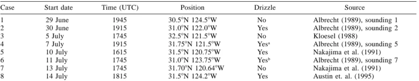
Table 1 summarizes the aircraft observations, taken from three published accounts of in situ aircraft mea-surements (Albrecht 1989; Nakajima et al. 1991; Austin
TABLE1. Trajectory parameters for the drizzle study.
Case Start date Time (UTC) Position Drizzle Source
1 2 3 4 5 6 7 8 29 June 30 June 5 July 7 July 10 July 11 July 13 July 14 July 1945 1915 1745 1915 1615 1745 1745 1815 30.58N 124.58W 31.08N 122.08W 32.58N 121.58W 31.758N 121.58W 31.58N 120.758W 31.08N 123.758W 31.708N 120.648W 31.58N 124.28W No Yes No Yesa Yes Yesb No Yes Albrecht (1989), sounding 1 Albrecht (1989), sounding 2 Kloesel (1988) Albrecht (1989), sounding 5 Nakajima et al. (1991) Albrecht (1989), sounding 7 Nakajima et al. (1991) Austin et. al. (1995)
aSignificant precipitation was observed 3 h later.
bSignificant precipitation was observed during this sounding.
FIG. 3. Parcel trajectories used in the drizzle study. The map grid shows latitude 308N and longitude 1208W; the California coastline runs diagonally across the upper-right corner of the map. With the exception of case 6, all trajectories run roughly parallel to the Cal-ifornia coast.
et al. 1995) and from the National Center for Atmo-spheric Research (NCAR) Electra observer notes (Kloe-sel et al. 1988), which we use as initial conditions. The annotations describing ‘‘significant’’ precipitation, which are based on the number concentration and mean radius of drizzle-sized drops, are from Albrecht (1989). We refer to the trajectories starting from the observa-tions in this table as the ‘‘drizzle trajectories,’’ and dis-tinguish between ‘‘precipitating’’ and ‘‘nonprecipitat-ing’’ trajectories on the basis of the in situ measurements summarized in the fifth column.
The geographic region in which satellite imagery is available limits the length of trajectories to about a day and a half, which is long enough for any consequence of drizzle to manifest itself on the evolution of cloud fraction. We use the Lagrangian technique to observe cloud evolution for 33 h, from sunrise on one day to sunset the next. In the presence of 2–4 m s21random
errors in analyzed winds, the uncertainty in parcel po-sition after 33 h is of order 250 km (Kahl and Samson 1986); we use this figure to determine the size of the mesoscale-sized regions extracted from the satellite im-agery, noting that turbulent velocity scales for horizontal mixing are typically of the same order of magnitude. The trajectories may be divided into three time periods: the day on which the initial conditions are obtained (day 1), the following day (day 2), and the intervening night-time hours.
As Table 1 shows, the aircraft observations charac-terizing precipitation in the cloud layers were made at a variety of times during the morning, ranging from 1615 to 1945 UTC (815 to 1145 PST). To account for the strong diurnal modulation of cloud properties, we compute each trajectory backwards in time from the time and place of the aircraft observation to a uniform time in the morning (815 PST, or 1615 UTC), then compute the parcel trajectory forward in time for 33 h, until late afternoon (1615 PST) the next day. Environ-mental information and cloud parameters are reported at half-hourly intervals along each trajectory.
Figure 3 shows the locations of the air parcel tra-jectories used in the drizzle study. With the exception of case 6, all trajectories run roughly parallel to the California coast. We neglect those portions of trajec-tories in which the trajectrajec-tories came within 125 km of the coastline (the last 6 h of case 4 and 9 h of case 7).
b. Characterizing environmental evolution
Figure 4 shows the temporal evolution of environ-mental conditions (sea surface temperature, 1000-mb wind speed, and lower tropospheric stability as de-scribed below) along each of the eight drizzle trajec-tories listed in Table 1. On the basis of wind speed and SST histories alone, the trajectories may be roughly segregated into two groups: cases 1, 5, and 6, which exhibit wind speeds less than 4 m s21and changes in
sea surface temperatures less than about 0.5 K over the 33-h period; and the other five cases, which exhibit higher wind speeds and larger sea surface temperature changes. (The total change in SST along trajectories 2
FIG. 4. (a) Wind speed, (b) sea surface temperature, and (c) lower tropospheric stabilityDu(defined in text) histories for the drizzle trajectories. SST is not reported for case 7 after the trajectory nears land. Cases 1, 5, and 6 are characterized by low wind speeds and smaller rates of change of sea surface temperature, whileDuincreases rather than decreases along trajectories 1 and 2.
and 4 is also small, but in both of these examples brief episodes of SST decrease offset the general increase of SST along the trajectory.) The fine spatial resolution of the SST grid and the small-scale variability in SST are responsible for the noisy evolution of SST along the trajectories, most visibly in case 8.
It has been known for almost a century that inver-sions in the lower troposphere promote the formation of stratocumulus and fog (Bristow 1952); Klein and Hartmann (1993) quantified this link by showing that the stratiform cloud fraction is related to stability of
the lower troposphere [defined asDu 5 u(700 mb)2
u(sea level pressure, T 5 SST)] on seasonal time-scales such that each 1-K increase in potential tem-perature differenceDu corresponds to a 6% increase in cloud fraction. The lowest panel of Fig. 4 shows the temporal evolution of Du along the drizzle tra-jectories, assuming that sea level pressure is constant at 1000 mb. The total range of stratification among the trajectories (about 6 K) is a significant portion of the global range on seasonal timescales, and the tem-poral change experienced along individual trajectories
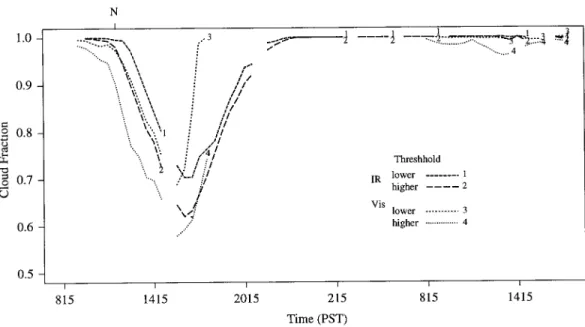
FIG. 5. Evolution of cloud fraction along case 1. Results from the VIS and IR techniques are shown using high and low threshold values. The letter N along the upper axis indicates the time of the aircraft sounding in which precipitation was not observed. This example is typical in that the VIS and IR measures of cloud fraction computed with similar threshold values agree reasonably well with one another and in that cloud fraction is near one at night.
(as much as 4 K) suggests that, if the mechanism linking cfandDuoperates on daily as well as monthly
timescales, average cloud fraction might be expected to change by as much as 25%. Note, however, that cases 1 and 2 experience increasing Du with time, while all other trajectories experience a decrease. c. Characterizing cloud evolution
The temporal evolution of cloud fraction for case 1 is presented in Fig. 5, where the ‘‘N’’ (for ‘‘no precip-itation’’) on the upper axis denotes the time of the in situ observation for this trajectory. Here we compute four measures of cloud fraction: using the IR technique with temperature thresholds of DT 5 3.25 and 4.5 K, and via the VIS technique with reflectance thresholds
DR50.03 and 0.10. As is typically true along this set of trajectories, estimates of cloud fraction made using the VIS and IR techniques are consistent. In this ex-ample, all measures show a large decrease in cloud frac-tion during the afternoon of the first day of evolufrac-tion, solid cloud cover during the nighttime hours, and a neg-ligible decrease on the afternoon of the second day. Differences between conservative (higher threshold) and more liberal estimates of cloud amount indicate the presence of optically thin clouds and/or partial cloudi-ness on scales smaller than the pixel size; this can be seen most clearly at 1615 PST on the first afternoon, when 10% of the total cloud cover falls into this cate-gory according the IR techniques and 30% according to the VIS methods. Gaps indicate data missing either due to failures in data collection or to the replacement of 11-mm imagery with 6.7-mm imagery.
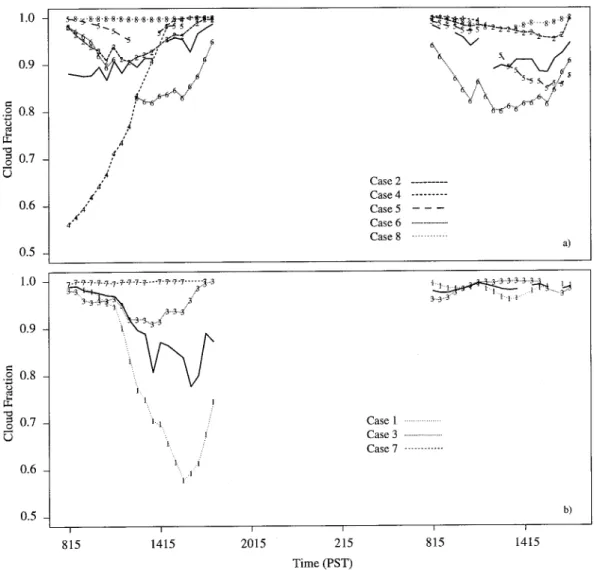
Figure 6 shows the evolution of cloud fraction during daytime hours for all eight drizzle trajectories as mea-sured by the VIS technique withDR50.10. (The more stringent threshold is used here to better detect marginal changes in cloudiness.) The upper panel shows the re-sults for those trajectories whose initial conditions in-dicated the presence of precipitation; the lower panel those in which the in situ observations indicated no precipitation. The thick solid lines in each panel indicate the average value of cloud fraction, which exhibits some noise because the number of cases at any given time varies. The low value of cloud fraction reported during the first day (7 July) of evolution of case 4 is deceptive. On this day, the aircraft flights were centered on a sharp transition between solid stratocumulus and entirely clear air (Betts and Boers 1990). The image series includes this edge, which gradually moves out of the field of view as the clear air fills with clouds. Note that, ex-cluding case 4, the only trajectory along which cloud fraction decreases below 80% during daylight hours is (nonprecipitating) case 1.
Nighttime cloud reformation can be seen in Fig. 7, which illustrates the evolution of cloud fraction for all trajectories obtained using the IR technique with
DT 5 4.5 K and the average cloud fraction at each hour. Along both precipitating and nonprecipitating trajectories cloud fraction is nearly unity during the nighttime hours, as is consistent with Eulerian ob-servations of the diurnal cycle of low cloud amount in this region (Minnis et al. 1992; Rozendaal et al. 1995). The IR cloud fraction estimate generally agrees well on a case-by-case basis with the VIS estimates, although some small reductions in cloud fraction
re-FIG. 6. Temporal evolution of cloud fraction obtained using the VIS technique along (a) the precipitating trajectories and (b) the nonprecipitating trajectories. The solid line in each panel indicates average cloud fraction, which is somewhat noisy due to variations in the number of images available at any one time. A high reflectance threshold value is used here to highlight marginal changes in cloudiness.
ported by the VIS technique are not detected by the IR technique (e.g., case 2 and 6 during the first af-ternoon of evolution). In contrast, the IR technique is sensitive to reductions in visible wavelength cloud optical depth, since clouds thinner than t ø 5 are semitransparent in the infrared. This is most evident on the first afternoon of evolution of case 7, when the IR technique reports cloud fraction dropping to almost 70%, while the VIS technique reports essentially solid clouds.
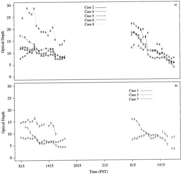
Figure 8 presents the temporal evolution of the me-dian value of cloud optical depth along the drizzle trajectories. Precipitation in stratocumulus clouds is generally observed to increase with cloud geometric thickness and cloud liquid water path (Nicholls and Leighton 1986) and average droplet size (Austin et al. 1995), while optical depth varies as the ratio of
liquid water path to drop size. In these eight examples,
tby itself is a poor indicator of the presence of pre-cipitation: although the two optically thickest clouds on the first morning (cases 8 and 5) are indeed pre-cipitating, the third and fourth thickest (cases 1 and 7) are not. Of note also are strong diurnal variations in optical depth evident for those clouds that have large optical depth in early morning hours; we return to this point in section 4.
Of particular note is (nonprecipitating) case 1, which is optically thick on the morning of the first day of evolution (optical depth about 13, ranked fourth of eight) but that thins dramatically and shows a marked decrease in cloud fraction by the middle of the first afternoon. The average boundary layer depth (not shown) is 1.4 km, about 200 m greater than the second deepest boundary layer and 300–400 m deeper than the
FIG. 7. Evolution of cloud fraction obtained using the IR technique along the (a) nonprecipitating and (b) precipitating drizzle trajectories. Although cloud fraction varies somewhat during daylight hours, cloud fraction is nearly one at night for all eight cases, regardless of the presence or absence of precipitation.
depth of the majority of layers in the drizzle study. As deeper boundary layers are generally less well coupled than shallower layers, it seems likely that the clearing on day 1 is due to solar absorption in a decoupled layer. Cloud fraction remains high during the second day of evolution for reasons that are not clear.
d. Discussion
Figures 6 and 7 show that cloud fraction exhibits relatively little variability along these eight trajectories. Cloud fraction is uniformly high at night and decreases only occasionally during daylight hours and then typi-cally only to around 80%. There is no systematic re-lationship in this very small set of examples between the presence or absence of precipitation as measured by the in situ aircraft and the downstream evolution of cloud fraction. In only one case does cloud fraction decrease below 0.8, and in situ observations on this day
showed no sign of drizzle. Some variability in cloud fraction is present along both precipitating and nonpre-cipitating trajectories, but neither the mean value nor the amount of variability is significantly larger in the precipitating than in the nonprecipitating trajectories, and the amount of variability between the two classes of trajectories is no greater than the differences typically seen between the various measurement techniques.
Cloud fraction decreases from unity on the first day of evolution in only two of our eight examples, one of which is precipitating. This implies that the water that is directly removed from the boundary layer by precip-itation is replenished by fluxes of vapor from the sur-face. Indeed, aircraft have observed this replacement in several case studies during FIRE (Paluch and Lenschow 1991; Austin et al. 1995). It is unclear whether models such as Albrecht’s (1989) treatment can adequately re-solve this approximate balance, given appropriate values of the relevant parameters.
FIG. 8. Temporal evolution of cloud optical depth along the drizzle trajectories. Precipitation and cloud optical depth both increase with cloud thickness, but cloud optical depth alone is a poor predictor of the presence or absence of precipitation in this dataset.
4. Assessing the importance of environmental state
In this section we identify typical patterns of diurnal evolution of cloud radiative properties and explore the links between those properties and the evolution of en-vironmental parameters in a Lagrangian frame of ref-erence. We do so by considering about 40 trajectories, establishing common patterns in the temporal evolution of the clouds along the trajectories, and assessing the degree to which the environmental evolution is asso-ciated with cloud evolution. The large number of tra-jectories we require means that supporting in situ ob-servations like those used in the drizzle study are not available, and so we must abandon the possibility of assessing the role of cloud microphysics.
We choose two starting positions in the FIRE region: 358N, 1258W and 358N, 127.58W, which are far enough apart that trajectories beginning at the two points are independent (in the sense that the images do not overlap)
but located such that most 33-h trajectories begun from these two points remain in the observation region. We compute parcel trajectories for 33 h forward in time beginning at 0815 PST from each of these positions for each of 23 days during FIRE. Eight of the 46 parcel trajectories are not acceptable either because large num-bers of consecutive satellite images are unavailable or because the trajectories run onshore during their evo-lution. As in section 3, we measure cloud fraction using two infrared and two visible thresholds.
a. Patterns of cloud evolution and their radiative consequences
Figure 9 documents the distribution of cloud prop-erties (median optical depth, boundary layer height, and cloud fraction averaged over all available measures) among the 38 trajectories as a function of local time.
FIG. 9. Evolution of cloud parameters (average cloud fraction, median optical depth, and boundary layer depth) among 38 trajectories. Solid lines show the mean value of each parameter at each hour; dashed lines show the first and third quartile values. These panels illustrate the amount of variability in the population, although no individual trajectory experiences the evolution shown here.
For each cloud property the figure shows the mean value (solid line) and the first and third quartile values at each hour. During nighttime hours, the mean cloud fraction is lower than the 75th percentile value (which is nearly unity), indicating that only a few trajectories experience nighttime cloud fraction less than 1. Further investi-gation reveals the nighttime behavior of cloud properties is quite consistent in this dataset, with 85% percent of all trajectories having cloud fractions greater than 95%. The temporal evolution described in Fig. 9 is not experienced by any single example, but represents the
hourly evolution of the entire population of trajectories. Therefore, we use principal component analysis (e.g., Dillon and Goldstein 1984) to identify common features in the temporal evolution of cloud parameters. Principal component analysis identifies those orthogonal patterns of variability that explain the greatest amount of vari-ance among all the variables at once by computing the eigenvectors of the covariance matrix. The eigenvectors (or component) are ranked in terms of their eigenvalues
li, which are normalized such that the sum of the ei-genvalues is equal to one; each component is then said
TABLE2. Quantities used to summarize daytime cloud evolution. These variables are used in the principal component analysis shown in Table 3.
Variable Definition Defined during
min(cf) Instantaneous minimum cloud fraction measured using either
VIS or IR technique with stringent thresholds
daylight hours range(cf) Range in cloud fraction averaged across two VIS and two IR
cloud detection methods
daytime hours cf Time mean of cloud fraction averaged across two VIS and two
IR cloud detection methods
daytime hours
range(t) Range in hourly median optical depth daytime hours
t Time average of hourly median optical depth of cloudy pixels 0800–1200 local time var(t) Variance of optical depth of cloud pixels normalized by median
optical depth
daytime hours zi Time average of hourly median boundary layer depth daytime hours
TABLE3. Principal components for cloud evolution during daytime hours. The loading indicates the projection of each variable onto the computed component. This pattern of evolution explains much of the variability in diurnal evolution in cloud radiative properties without reference to the environment to which the clouds are subject.
All variables Day 1 Day 2 Neglectingz ,i var(t) Day 1 Day 2 % of var 51.2 57.5 71.7 76.1 Loadings: min(cf) range(cf) cf range(t) t var(t) zi 0.483 20.438 0.470 0.430 0.410 ,0.100 ,0.100 0.476 20.461 0.431 0.421 0.365 20.227 0.139 0.482 20.439 0.468 0.431 0.412 0.488 20.476 0.440 0.444 0.380 to account for li 3 100% of the total variance in the dataset. We estimate the statistical significance of each component with a Monte Carlo test [Overland and Pre-isendorfer (1982); note also ‘‘Rule N’’ in PrePre-isendorfer and Mobley (1988)]. Given the unvarying nighttime be-havior along these trajectories, we focus on the daytime evolution of cloud properties, which we summarize us-ing the variables detailed in Table 2.
Of the principal components computed from these seven variables measured across our 38 cases, only the first is statistically significant. This component (com-puted separately for each day) is shown in Table 3, which indicates the amount of variance explained and the projection of each variable onto the component. The pattern is quite similar on both days: large values of morning optical depth are associated with a wide range in optical depth, high average cloud fraction, high min-imum cloud fraction, and small range in cloud fraction. On the second day this pattern is also loosely correlated with deeper boundary layers and smaller variability in optical depth. If we compute the principal components without including boundary layer depth or optical depth variability, the patterns for days 1 and 2 are nearly iden-tical. We focus below on this second set of principal components.
The physical interpretation of this pattern is clear and
unsurprising: clouds that are optically thick in the morn-ing hours are likely to show a large variation in optical depth but are likely to remain unbroken. Since the prin-cipal component is arbitrary with respect to sign, the converse is also true: clouds that are optically thin in the morning are likely to break up without showing a large variation in optical thickness.
The scalar product between the principal component and the variables measured for a given trajectory de-termine the score or projection along the principal com-ponent for that trajectory. Individual trajectories with high positive scores along the component we have iden-tified, therefore, will be optically thick in the morning and likely to remain solid during the day. This is illus-trated in Fig. 10, which shows the daytime evolution of cloud properties for the trajectories that have the lowest, highest, and quartile projections along the principal component on each day. (Note that near-zero scores along the principal component may indicate either that the clouds are of moderate optical depth and show a moderate amount of variability in cloud fraction, or that they exhibit a very different pattern in variability, such as optically thick clouds with a large diurnal range in cloud fraction.) We stress that this pattern of evolution alone accounts for more than 70% of the variability (excluding measures of boundary layer depth or optical depth variability) among all 76 diurnal cycles (38 cases spanning 2 days each) observed in the study without regard to environment in which the clouds are evolving. The relationship between cloud ‘‘breakup’’ [i.e., low values of min (cf) along with high values of range(cf)]
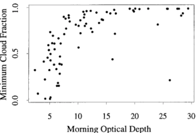
is amplified in Fig. 11, which shows the minimum day-time value of cloud fraction as a function of average (over morning hours) cloud optical depth. Clouds with small values of morning optical depth exhibit wide vari-ability in the minimum cloud fraction, but a threshold is also clear: clouds with median optical depth greater than about 10 are quite unlikely to break up.
HOW DOES DIURNAL VARIABILITY AFFECT CLOUD RADIATIVE FORCING?
Marine boundary layer clouds cause a substantial per-turbation to the surface and top-of-atmosphere (TOA)
FIG. 10. Evolution of cloud parameters along individual trajectories. Table 3 details the principal component that describes the variability in cloud evolution. Trajectories having high positive scores along the component exhibit large morning optical depths and little likelihood of breaking up during the day. Here the evolution along those trajectories with the lowest (line 1), highest (4), and first and third quartile scores (2 and 3) is shown.
radiation budgets. Our identification of typical patterns of the diurnal evolution of cloud radiative properties allows us to assess the degree to which computations that ignore this temporal variability may be in error. Table 4 shows the diurnally averaged cloud radiative forcing (e.g., Charlock and Ramanathan 1985) for three patterns of diurnal variability: a composite of the three trajectories with the lowest principal component score on day 1 (clouds that are optically thin in the morning and likely to break up during the day), a similar com-posite for clouds with the highest scores, and ‘‘average
clouds,’’ defined as the mean across all 38 trajectories. Hourly values of cloud fraction and cloud optical depth are determined for each cloud type, with missing values (including nighttime optical depth) filled by linear in-terpolation in time. The diurnal cycle of solar insolation is representative of 1 July at 308N, 1308W. Total (short-wave and long(short-wave) cloud radiative forcing at the top of the atmosphere and the surface is computed using a spectrally resolved radiative transfer model incorporat-ing scatterincorporat-ing by molecules and cloud droplets, extinc-tion by aerosols, and absorpextinc-tion by gasses (Key 1996).
FIG. 11. Minimum cloud fraction during daylight hours as a func-tion of average cloud optical depth during morning (0800–1200 PST) hours. Clouds with morning optical depth greater than about 10 are unlikely to reach cloud fractions less than 80%, regardless of envi-ronmental changes. Two data points showing high optical depth and low minimum cloud fraction are associated with optically thick clouds close enough (about 625 m) to the ocean surface to be considered as clear by the stringent infrared detection threshold.
TABLE4. Cloud radiative forcing under various approximations for typical patterns of the diurnal evolution of cloud optical depth and cloud fraction. Diurnally averaged cloud radiative forcing (W m22) is computed using the hour-by-hour values. The absolute difference
between this time-resolved calculation and results computed holding either or both of cloud fraction and cloud optical depth fixed at its diurnal average is also shown; relative differences (%) are indicated in parentheses. The degree to which an individual trajectory may be classified as ‘‘thick’’ or ‘‘thin’’ is much more important than efforts to resolve the diurnal cycle.
Thin clouds TOA Surface Average clouds TOA Surface Thick clouds TOA Surface Varyingt, cf 230.8 25.0 2117.5 286.2 2190.4 2168.8
Absolute and relative (%) differences from diurnally resolved calculation Fixedt Fixed cf Fixedt, cf 0.3 (21.1) 2.32 (9.5) 23.7 (10.6) 0.1 (22.2) 27.5 (60.2) 23.7 (62.0) 0.5 (20.4) 21.3 (1.1) 21.0 (0.8) 0.8 (20.9) 22.5 (2.8) 21.9 (2.2) 24.5 (2.3) 22.0 (1.0) 26.7 (3.4) 26.2 (3.6) 22.4 (1.4) 28.8 (4.9) Cloud radiative forcing computed using diurnally
varying cloud fraction and cloud optical depth is com-pared in Table 4 with the forcing calculated holding cloud optical depth and/or cloud fraction fixed at their diurnal average. Neglecting the diurnal cycle in cloud fraction has the largest impact for thin clouds, which show the largest amount of variability in cloud fraction: the 9.5% TOA error relative to the diurnally resolved calculation is similar to that reported by Rozendaal et al. (1995) at 308N, 1408W. The diurnal variation in cloud optical depth, on the other hand, has the greatest impact on thickest clouds, causing a 4.5 W m22 difference.
What is most striking, however, is that the differences between calculations of cloud radiative forcing that do and do not account for diurnal changes in cloud radiative properties are minuscule compared to the differences in the forcing caused by different types of clouds. b. Patterns of environmental evolution
Figure 12 shows the hour-by-hour evolution of en-vironmental properties averaged across the collection of
38 trajectories. Sea surface temperature increases and wind speed decreases slightly as the parcels are advected towards the southwest. Day-to-day variability in upper tropospheric temperature causes a large range in Du among the trajectories, although the mean and quartile values vary relatively little with time.
Principal component analysis (not shown) of the en-vironmental parameters reveals that trajectories that ex-perience higher average wind speeds are more likely to show higher average sea surface temperatures. This is consistent with the small initial range in SST and the tendency of parcels to advect towards warmer sea sur-face temperatures. Indeed, the best correlation between SST and wind speed occurs when SST in the last hours of the trajectory is correlated with wind speed during the initial hours. It also implies that individual histories with higher SSTs towards the end of their evolution have experienced a larger average rate of change of SST. Lower tropospheric stability, on the other hand, is driven primarily by 700-mb temperature along each trajectory and thus is largely uncorrelated with SST and wind speed.
c. Links between environmental parameters and cloud response
We assess the degree to which the diurnal evolution of cloud radiative properties is determined by the en-vironment in which the clouds evolve by looking for systematic relationships between cloud response (as measured by the score on the principal component we have identified) with various environmental parameters. Since boundary layer depth is thought to be important in determining the amount of decoupling in the bound-ary layer, it plays a dual role in this discussion: as both a measure of the state of the environment and as a sec-ond response (separate from the diurnal behavior in-dicated by the principal component analysis) the cloud system can have.
We begin by considering contemporaneous rela-tionships between cloud and environmental parame-ters. For both 10-h daylight periods, we compute the average wind speed, boundary layer depth, sea surface temperature, and lower tropospheric stability for each
FIG. 12. Environmental parameters averaged among trajectories. Trajectories that are subject to high wind speeds early in their evolution are likely to have higher than average sea surface temperatures later in their evolution. The variation of lower tropospheric stability is much larger between trajectories than along individual trajectories. trajectory. None of these variables are well correlated
with the principal component scores for the trajec-tories during the same period. The only statistically significant correlation (r5 0.46) is betweenDuand the principal component score, indicating that more stable boundary layers are likely to contain thick clouds. Although lower tropospheric stability is thought to act on cloud properties in part through its influence on boundary layer depth, the lack of cor-relation between cloud response and boundary layer depth is to be expected, since boundary layer depth
was included in the set of variables used to derive the principal component but was not picked out by the analysis. The low correlation coefficient obscures a relationship between boundary layer depth and cloud behavior, however. Figure 13 shows average morning optical depth as a function of average boundary layer depth. Although clouds shallower than 1.25 km (about 75% of the population) show a wide range in morning optical depth, none of the clouds in deeper boundary layers maintain a morning average optical depth greater than 15. Nonetheless, these deep boundary
FIG. 13. Average morning optical depth as a function of average boundary layer depth. Boundary layers deeper than 1.25 km do not exhibit cloud optical depths greater than 15.
layers exhibit both a range of both positive and neg-ative scores along the principal component.
As we have emphasized, time delays may exist be-tween the time an environmental parameter changes and the time the effect of that change is manifest in cloud properties. We assess the degree to which cloud response is correlated with environmental parameters at prior times by correlating instantaneous values of sea surface temperature, wind speed, stability, and boundary layer depth at each hour along the trajectory with the cloud response on day 2 (measured by the principal component score). These correlations are shown in Fig. 14, along with 95% and 99% confidence intervals (dark and light shaded horizontal boxes, re-spectively). Lower tropospheric stability is signifi-cantly correlated with the principal component score at all hours, indicating that broader variations in sta-bility exist within the group of trajectories than along individual examples. The correlation increases with time lag to a broad maximum during the first 8 h of the trajectory, 16–24 h prior to the cloud response; this increase is itself statistically significant at the 96% level. Sea surface temperature is correlated at about the 95% level during the cloud response period and the 12 h prior, while the correlation between cloud response on day 2 and wind speed during the early part of the trajectory reflects the role of wind speed in driving SST. Boundary layer depth is significantly negatively correlated with cloud response only with a 20–25 h lag.
Conceptual models of stratocumulus dynamics (e.g., Wyant et al. 1997) indicate that boundary layer depth plays an important role in controlling cloud fraction, and we saw in Fig. 13 that values of zi greater than
about 1.5 km are associated with limited average cloud optical depth. This prompts us to investigate to what extent boundary layer depth is determined by environ-mental conditions along a trajectory. Figure 15 shows the time-dependent correlation of sea surface tempera-ture,Du, and wind speed with average boundary layer
depth during day 2 (hours 25–34). As we might expect, boundary layer depth during day 2 is correlated with SST and anticorrelated withDuat previous times along the trajectory, while wind speed is uncorrelated with zi
at all times. The temporal behavior of the correlation with SST is somewhat puzzling, going through a sta-tistically significant minimum for about 8 h. The tem-poral changes in correlation withDuare not statistically significant.
d. Discussion
We have identified a robust pattern in the temporal evolution of cloud radiative properties (cloud fraction and optical depth) in the FIRE region. In this dataset, the morning value of cloud optical depth determines to a large extent whether or not a cloud deck will break up during the course of the day (where breakup is de-fined using several measures of the temporal evolution of cloud fraction). A threshold optical depth value of roughly 10 is significant: clouds with average optical depth greater than this value during morning hours are quite unlikely to exhibit cloud fraction less than 80% at any time during the day. This behavior is consistent with our understanding of the role of solar radiation in determining boundary layer cloud fraction. Clouds may be optically thick either because they contain small drops and so absorb little near-infrared radiation, or be-cause they contain large amounts of liquid water; in either case clouds will be unlikely to break up. Our radiative calculations indicate that day-to-day differ-ences in morning cloud optical depth and the resultant susceptibility to breakup play a key role in determining the magnitude of cloud radiative forcing at both the surface and the top of the atmosphere.
The link between morning optical thickness and the likelihood of cloud breakup in the FIRE region also implies that an exclusive focus on the diurnal variability of cloud fraction tells only part of the story. We propose that diurnal cycles of cloud fraction reflect an underlying variation in cloud liquid water such that solar heating and changes in boundary layer dynamics lead first to a reduction in cloud optical depth, then to a decrease in cloud fraction. Such a view is consistent with the ob-servation that the diurnal cycle in cloud fraction is larg-est downwind of regions in which cloud fraction is greatest (Rozendaal et al. 1995). Composite diurnal cy-cles showing large variation in both cloud fraction and optical depth (e.g., Minnis et al. 1992) may be under-stood as an average over days containing thick and thin clouds.
Our analysis suggests that several environmental fac-tors experienced along a trajectory play a role in con-trolling the optical thickness and susceptibility to di-urnal breakup of marine boundary layer clouds. Trajec-tories experiencing higher sea surface temperatures (and faster rates of change of SST) are likely to produce thicker, more robust clouds. This correlation is
signif-FIG. 14. Correlation between cloud response on day 2 (hours 25–34, shown as a shaded vertical rectangle) and instantaneous values of environmental parameters (sea surface temperature, lower tropospheric stability, boundary layer depth, and wind speed) as a function of time. The dark and light shaded horizontal boxes delimit 95% and 99% percent confidence limits, respectively. Cloud response is marginally well correlated with SST during the prior 12 h and withDuover longer timescales such that rapid changes in SST and high values of stability lead to thicker, more robust clouds.
FIG. 15. Correlation between average boundary layer depth on day 2 and instantaneous values of sea surface temperature, lower tropospheric stability, and wind speed as a function of time. The dark and light shaded horizontal boxes indicate 95% and 99% percent confidence limits, respectively.
icant at about the 95% level and applies during the period during which cloud response is measured and for as many as 12 h before. Higher rates of change of sea surface temperatures are likely to promote cloudiness by increasing air–sea mixing, including mixing asso-ciated with cumulus convection, which provides a source of cloud water that counteracts the drying effects of entrainment and absorption of solar radiation. Breth-erton and Wyant (1997) indicate that buoyancy fluxes associated with high sea surface temperatures eventually lead to decoupling, but we suspect that the boundary layers in our sample are shallow enough (mostly 1.25 km or less) that mixing and cumulus convection are quite effective in providing water to the stratiform cloud layer even in those boundary layers that are decoupled
from the surface. That the link between SST and cloud response is strongest during the day on which cloud properties are measured and the night before is consis-tent with our understanding of the equilibration time for water in the boundary layer.
A second link exists between lower tropospheric sta-bility and morning cloud optical thickness. The corre-lation is strongest given a 16–24 h or greater lag between the measurement ofDu and cloud response, but since
Duvaries relatively little along a given trajectory the correlation is robust at all times. Although decreases in
Duare likely to increase entrainment and hence bound-ary layer depth over time, we find in this dataset no direct relationship between zi on a given day and the
and robust. This too may be a consequence of robust ocean–atmosphere coupling in the generally shallow boundary layers in our dataset, since we find that bound-ary layers deeper than 1.25 km show a smaller variation in morning cloud optical thickness than the rest of our sample. Boundary layer depth is correlated with cloud response given an 18–24 h delay; we believe that this link is incidental. Because cloud response is correlated withDubut not with zi on daily timescales, it is clear
that the influence of stability on cloud properties is not limited to its role in controlling boundary layer depth. It appears that boundary layer depth is determined in part both by sea surface temperature and lower tropo-spheric stability at all times along the trajectory. This correlation is in accordance with our understanding of the manner in which these factors influence entrainment. The insensitivity of the correlations of SST andDuwith boundary layer depth to the time separating the mea-surements may reflect both the long timescales associ-ated with entrainment changing boundary layer depth as well as the consistence of upper tropospheric tem-perature along individual trajectories.
Klein et al. (1995) identified a 24–36 h timescale over which SST and lower tropospheric stability influence cloudiness in deeper marine boundary layers, and they associated this delay with the time necessary for the temperature and moisture content of the boundary layer to adjust to changes in environmental conditions. In our dataset the timescales are somewhat shorter (12 h for SST and 16–24 h forDu), which is consistent with the smaller boundary layer depths in our study. The dif-ferent timescale for the influences of SST andDumay reflect the relative ease with which fluxes from the ocean surface can modify the boundary layer as compared to entrainment: in a mixed layer model subject to boundary conditions typical of the eastern Pacific, for example, surface flux transfer velocities are roughly twice as large as entrainment velocities.
5. Conclusions
These studies have been based on data taken from the FIRE region off the coast of California, which is char-acterized by shallow boundary layers, high average cloud fraction, low diurnal variability in cloud fraction, large subsidence, and winds blowing steadily across SST gradients such that parcels experience about 1.5 K per day of warming. In a climatological sense, this is the region upstream of the maximum in diurnally av-eraged cloud fraction. Similar regimes occur in other parts of the eastern subtropical oceans, most notably off the coasts of Namibia, Chile, and to some extent near the Azores (Klein and Hartmann 1993). We expect that the insensitivity of cloud fraction to the presence of precipitation, as well as the relationships we have de-scribed between the rate of SST change, morning cloud optical depth, and the diurnal variability of cloud frac-tion apply more or less unchanged to these regions. Our
results may also illuminate the behavior of boundary layer clouds in other regimes, although insight into the processes driving the stratocumulus to cumulus transi-tion is necessarily indirect.
Our sparse set of Lagrangian observations do not sup-port the hypothesis that precipitation alone plays a lead-ing-order role in controlling boundary layer cloud frac-tion in regions of high average cloudiness. In our very small set of examples, the effects of precipitation on cloud fraction are masked by the much more important role of solar insolation. This study does not rule out the possibility that precipitation may be important in other regimes, however. In particular, we are unable to address the question of whether precipitation is important in modifying the stratocumulus to trade cumulus transition, where deeper boundary layers and more tenuous cloud– ocean coupling may allow precipitation to play a more central role.
We have shown that rapid increases in sea surface temperature are associated with thicker clouds that are less likely to break up over the course of the day. This contrasts with models (Krueger et al. 1995; Wyant et al. 1997) of the stratocumulus to cumulus transition in which higher SSTs are linked with deeper, more un-coupled clouds. We suggest, therefore, that sea surface temperature may play two distinct roles in helping to determine cloudiness in the marine boundary layer. Rap-id increases of sea surface temperature give rise to large fluxes of heat and moisture from the sea surface into the boundary layer and help to promote convection (ei-ther directly or through the generation of conditional instability) and cloudiness. On the other hand, larger sea surface temperatures are linked to deeper boundary layers and hence lower average values of cloud fraction through buoyancy fluxes and entrainment. The two mechanisms may generate two Lagrangian timescales for marine boundary layer cloudiness: a timescale of several days or more corresponding to the influence of SST on boundary layer depth, and the approximately 24 h timescale identified by Klein et al. (1995) and confirmed here, corresponding to the length of time nec-essary for environmental conditions to influence bound-ary layer energy and moisture content. We surmise that rapid changes in SST are likely to be associated with larger values of boundary layer cloudiness across the stratocumulus to cumulus transition on day-to-day time-scales and that this influence will be clear along indi-vidual Lagrangian trajectories.
Boundary layers nearer to the stratocumulus to cu-mulus transition are generally deeper and the cloud layer more loosely coupled to the ocean surface than in our examples. Under these conditions we expect that the morning value of cloud optical depth will continue to influence the diurnal variability in cloud properties but that cloud optical depths will decrease on average, lead-ing to more frequent breakup. We also suspect that the threshold value of optical depth necessary for clouds not to break up will increase with boundary layer depth