Vol. 58, No. 1, January 2012, pp. 78–93
ISSN 0025-1909 (print)ISSN 1526-5501 (online) http://dx.doi.org/10.1287/mnsc.1110.1348
© 2012 INFORMS
The Impact of Gender Composition on
Team Performance and Decision Making:
Evidence from the Field
Jose Apesteguia
ICREA, Universitat Pompeu Fabra and Barcelona Graduate School of Economics, 08005 Barcelona, Spain, jose.apesteguia@upf.edu
Ghazala Azmat, Nagore Iriberri
Universitat Pompeu Fabra and Barcelona Graduate School of Economics, 08005 Barcelona, Spain {ghazala.azmat@upf.edu, nagore.iriberri@upf.edu}
W
e investigate whether the gender composition of teams affects their economic performance. We study a large business game, played in groups of three, in which each group takes the role of a general manager. There are two parallel competitions, one involving undergraduates and the other involving MBA students. Our analysis shows that teams formed by three women are significantly outperformed by all other gender combinations, both at the undergraduate and MBA levels. Looking across the performance distribution, we find that for undergraduates, three-women teams are outperformed throughout, but by as much as 0.47 of a standard deviation of the mean at the bottom and by only 0.09 at the top. For MBA students, at the top, the best performing group is two men and one woman. The differences in performance are explained by differences in decision making. We observe that three-women teams are less aggressive in their pricing strategies, invest less in research and development, and invest more in social sustainability initiatives than does any other gender combination.Key words: gender; teams; performance; decision making
History: Received July 14, 2010; accepted February 11, 2011, by Brad Barber, Teck Ho, and Terrance Odean, special issue editors. Published online inArticles in AdvanceJune 20, 2011.
1.
Introduction
Gender differences and their impact on economic out-comes have attracted increasing attention, both in the media and in the economic literature. There is evidence for systematic differences in the origins of choice and behavior by gender, namely, in the prefer-ences of men and women. Croson and Gneezy (2009, p. 1), in a comprehensive and exhaustive review of the work on gender differences in economic experi-ments, summarize the findings as follows: “We find that women are indeed more risk averse than men. We find that the social preferences of women are more situationally specific than those of men; women are neither more nor less socially oriented, but their social preferences are more malleable. Finally, we find that women are more averse to competition than are men.”1
The gender difference in risk attitudes, social pref-erences, and preferences over competitive
environ-1See also Andreoni and Versterlund (2001), Byrnes et al. (1999),
Charness and Gneezy (2007), Croson and Buchan (1999), Gneezy et al. (2003), and Niederle and Vesterlund (2007).
ments has important implications for the understand-ing of differences in economic and social outcomes. Two prominent issues that have recently been con-nected to gender differences in preferences are the gender gap in labor markets (Bertrand and Hallock 2001, Bertrand et al. 2010, Manning and Swaffield 2008) and the influence of women in human develop-ment (Miller 2008).
The studies on gender differences are most com-monly done at the individual level, despite important decisions in modern economies often being made by groups or teams. Committees and boards, business-partners, and even industrial and academic research groups are only a few examples of group decision making in the real world. Interestingly, the recent financial crisis has brought media attention to the gen-der composition of boards and its influence on the firms’ performance.2 The extrapolation of the
find-ings at the individual level to the group level is not, however, immediately apparent. It is well known that groups have their own idiosyncrasy. For example, a
2See, for example, Walker (2008) and Kristof (2009).
widely documented phenomenon is group polariza-tion, whereby groups make more extreme decisions than the average of the individual views in the group (see Stoner 1968).3 Therefore, the influence of gender
on group performance and decision making deserves greater attention. This is the focus of this paper.
Dufwenberg and Muren (2006) are a prominent exception in the experimental economics literature because they study the influence of gender compo-sition on group decisions. In a dictator game set-ting, they find that groups are more generous and equalitarian when women are the majority. They also find that the most generous groups are those with two men and one woman. In the field, Bagues and Esteve-Volart (2010) show that the chances of suc-cess of female (male) candidates for positions in the Corps of the Spanish Judiciary are affected by the gender composition of their evaluation committees. They find that female candidates have better chances of success with more males on the committees (see also Zinovyeva and Bagues 2010). Delfgaauw et al. (2009) study the interaction between the managers’ gender and the gender composition of the workers. They find that sales competition is effective only in stores where the store’s manager and a large frac-tion of the employees have the same gender. Finally, there are also empirical papers in finance that docu-ment a positive relationship between gender diversity in boardrooms and company performance. However, reverse causality is a pervasive problem in these stud-ies, because companies that perform better are quite likely to be companies that also focus more on the gender diversity of their boards (see Carter et al. 2003, Farrell and Hersch 2005, Adams and Ferreira 2009).
In this paper, we explore the influence of the team gender composition on economic performance. We study a large online business game, the L’Oréal e-Strat Challenge, which is played by groups of three. Teams play the role of a general manager of a beauty-industry company, competing in a market composed of four other simulated companies. There are two identical competitions occurring in paral-lel, one involving undergraduate students and the other involving MBA students. The L’Oréal e-Strat Challenge was designed to simulate real business decisions; hence, teams must take decisions related to brand management, research and development (R&D), and corporate responsibility initiatives. The winning teams receive a 10,000 euros prize, plus a paid trip to Paris. Perhaps even more importantly, winning candidates have the possibility of being hired
3See also Sobel (2006) for a theoretical account and for references to
the empirical literature. For other established differences between individuals and teams, see, e.g., Charness and Jackson (2007) and Charness et al. (2007).
by L’Oréal. Our database consists of the last three edi-tions of the L’Oréal e-Strat Challenge, from the years 2007, 2008, and 2009, yielding a total of 37,914 partic-ipants, organized into more than 16,000 teams from 1,500 different universities that are located in around 90 different countries around the world.
The L’Oréal e-Strat Challenge offers a unique setting to study the influence of the gender com-position of teams on performance and on decision making. First, it is played worldwide, by a large num-ber of individuals, coming from a large numnum-ber of different institutions. Second, there are two separate competitions, involving two different subject pools, undergraduate and MBA students. Each subject pool constitutes relevant samples to study the influence of gender composition of teams. The former repre-sents a subject pool that is close to the one typically used in the experimental economics literature. This may facilitate comparisons of established results at the individual level with new findings that emerge here at the group level. MBA students are also rele-vant because they represent a unique and important sample. These are subjects that, with a high prob-ability, will play a key role in real-world business management. Hence, it is relevant to understand how these subjects interact in groups, conditioning on the gender composition in teams. Third, we can study the effect of the gender composition on performance and on other important aspects such as specific busi-ness decisions. Fourth, as mentioned, the game aims to simulate the business environment as close as pos-sible to the real world. Finally, this study also offers an important advantage over existing empirical stud-ies. In particular, reverse causality is less of a concern here. Teams are formed before their performance and, more importantly, remain fixed over the entire game. Our analysis shows that teams formed by three women are significantly outperformed by any other gender combination, in both the undergraduate and MBA competitions. The magnitudes are sizable, about 0.18 of a standard deviation from the mean for the undergraduate students and about 0.17 for the MBA students. We show that these findings are robust after controlling for a number of important variables, such as the quality of the institutions, fields of study, and geographical areas.
When we extend our analysis to consider the distributional effects, we find that the performance of three-women teams shows interesting variations along the distribution. In the undergraduate competi-tion, although the underperformance of three-women teams remains significant along the entire distribu-tion, there is a marked decrease as we move to the right on the performance distribution. Among the lowest 10%, three-women teams are outperformed by as much as 0.47 of a standard deviation from the
mean, whereas at the top 20%, three-women teams are outperformed by only 0.09. We also find evidence that the optimal gender composition along the whole dis-tribution is that of two men and one woman, although the differences are not statistically significant. In the MBA competition, the performance levels of all the gender combinations are higher than that of three-women teams along the entire distribution, although the differences are not always significant. Interest-ingly, at the top 10%, the team composed of two men and one woman shows to be the optimal gender combination.
After establishing the differences in performance, we seek to understand which decisions drive these differences. First, we find that three-women teams invest significantly less in R&D, both in the under-graduate and MBA competitions. A possible inter-pretation of these differences is that three-women teams are more conservative in their management vision. Second, teams differ in their decisions related to another crucial aspect for performance, namely, brand management. In both competitions, three-women teams show significantly lower profits. We identify an important difference in the pricing strat-egy that leads to these differences: three-women teams are pricing their products higher than any other gender combination. That is, these teams are signifi-cantly less aggressive in their pricing strategies, and this has consequences on sales, on profits, and ulti-mately on economic performance. Finally, we observe differences in decisions related to corporate responsi-bility. We find that in both competitions, three-women teams invest significantly more in social initiatives than does any other gender composition.
Although many of our results can be interpreted as being in line with established results in the literature on individual gender differences, we also find new results, which are idiosyncratic to the team level. First, although we do find that three-women teams perform worse than other teams, we do not find any evidence for a monotonic relationship between the number of men in the team and their performance, such that teams with one man and three men are not different. Moreover, we find evidence that the best gender com-position of a team is two men and one woman. In particular, for MBA students our distributional anal-ysis shows that for the top 10% of the distribution, the two men and one woman combination is highly significant.
In our setting, because teams are not exogenously formed, there are competing explanations for the find-ings we report. It is important to consider and iden-tify the main driving force because the policy, social, and scientific conclusions are very different depend-ing on the explanation. In the final section, we discuss at length the potential explanations.
The rest of this paper is organized as follows. In §2, we introduce the L’Oréal e-Strat Challenge. Section 3 is devoted to the presentation of the demographics in our data. Section 4 establishes the main result on the effect of gender composition on performance. Sec-tion 5 is devoted to the understanding of where the performance differences come from. In §6, we discuss alternative explanations for our findings.
2.
The Game: L’Oréal e-Strat
Challenge
2.1. Overview of the Game
The L’Oréal e-Strat Challenge is one of the biggest online business simulation games. It was designed by StratX for L’Oréal. The game was launched in 2000, and since then there have been more than 250,000 participants from more than 2,200 institutions spread all over the world. It is open to all students in their final or penultimate year of undergraduate study, or studying an MBA, registered at a university anywhere in the world. Undergraduate and MBA students par-ticipate in separate competitions of the same game. All team members must attend the same university and must provide the following information: name, official ID, age, gender, university, field of study, and country of origin. Teams that do not comply with these requirements are discarded.
The game is played by teams of three members. Each of the teams plays the role of a general man-ager of a beauty-industry company, competing in a market composed of four other simulated compa-nies. That is, the participating teams do not compete with one another in the same market. The game was designed to simulate real business decisions. In turn, teams make decisions that are related to R&D, brand management, and corporate responsibility initiatives. The rules of the game are clearly stated in the detailed instructions. A proper understanding of the instruc-tions requires a good deal of time and effort.4 The
game is comprised of six rounds, plus a final round that is in a different format. The main performance variable is the stock price index(SPI), which measures the market value of the company, as a consequence of team’s decisions, as well as the decisions taken by the competing (simulated) firms. As such, the SPI is not only determined by current profits alone but also by broader management decisions that may be exploited in the future, such as investment in R&D.
The initial conditions are identical for all partici-pating teams. Subsequently, after decisions are taken in round one, the SPI is computed and only the best 1,700 participating teams in terms of their SPI are
4The instructions from the 2008 edition are available from the
selected to pass to the second round, taking into account country and zone quotas. The winning teams in the final round, one undergraduate team and one MBA, are awarded with a 10,000 euros prize each. Perhaps more importantly, they have the opportu-nity to meet high profile professionals at L’Oréal, and some of them are offered employment opportunities. In this paper, for an evenhanded comparison across teams, we will use data from the first round only. The starting situation in round one is exactly the same for all teams; therefore, the decisions and associated performances in the first round are fully comparable across teams. This is not the case for other rounds because teams’ performance depends on their game history.
2.2. Management Decisions
We distinguish between three different types of deci-sions that teams must undertake. These decideci-sions gen-erate what we refer to as midway outcome variables that in turn affect the final, and most important, out-come variable, the SPI.
First, teams make decisions regarding the invest-ment in R&D. Teams have an R&D departinvest-ment, where researchers discover two new formulae. These formulae should be interpreted as innovations that, if developed, can be used to create new brands or improve the existing ones. Teams must then make two main decisions. First, teams must decide whether to invest in zero, one, or two formulae. Second, if they decide to invest in any formula, they must spec-ify the amount that they wish to spend. These deci-sions form the midway outcome variable, namely, total R&D investment.
Second, teams must manage their brands. All teams start with the same two brands. Brands differ in their characteristics to target a specific customer profile. Participants know whether the brand is targeting high earners; affluent families, medium income families, low-income singles, or low-income families. In each edition, there are different brand targets for each of the two brands. The two main decisions that teams must make are the price and the production level for each of the two brands. These, in turn, influence the main midway outcome variables regarding the brand management, which are composed of sales, revenues, production costs, and inventory costs. Finally, these variables determine profits.
Third, teams must decide how much to invest in social and environmental initiatives. The former includes initiatives such as having health programs or continuous learning plans for employees. The envi-ronmental initiatives include actions such as using renewable raw materials, reducing water consump-tion, or having safety and health compliant plants. Teams’ investment in these initiatives determine
the social sustainability and environmental sustainabil-ityindices, which are the main two midway outcome variables in this area.
Overall, the decisions made in all three of these areas affect the market value of the company, and this is incorporated in the main performance variable, the SPI.
2.3. Data and the Relation Between Managerial Decisions and Performance
Our database consists of the last three editions of the L’Oréal e-Strat Challenge from the years 2007, 2008, and 2009. This includes a total of 37,914 participants from 1,500 different universities, located in about 90 different countries around the world.5
Success in the L’Oréal E-Strat Challenge, repre-sented by high values in SPI, is determined by the midway outcome variables and ultimately by teams’ management decisions. In this section, we elaborate on the relationship between decision variables, mid-way outcome variables, and the final performance variable, the SPI. This will facilitate the understanding and interpretation of the team differences in perfor-mance. We look at the associations across variables in two ways.
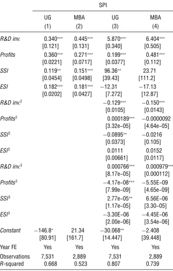
First, we show that there exists a relationship between the midway outcome variables and the SPI. We use a simple regression analysis, where we relate the final performance measure, the SPI, to the mid-way decision variables, separately for the two compe-titions, undergraduate and MBA students. The results are shown in columns (1) and (2) of Table 1. For both competitions, all the midway outcome variables are positively and significantly related to SPI. We also estimate these regressions for each of the edi-tions separately and we find qualitatively the same results; see Table A.3 in the online appendix, avail-able on the authors’ websites (http://www.econ.upf .edu/∼{apesteguia, azmat, iriberri}). When we run regressions separately for each of the midway out-come variables to SPI, shown in Table A.4 in the online appendix, we see that there are large differ-ences in the importance of each variable. The val-ues for the R-squared show that, not surprisingly, most of the variation in SPI is explained by the
5About 55% of the registered teams do not participate in the game,
such that there is attrition. More importantly, we find that there are no significant differences in attrition across different gender combi-nations. For the undergraduate competition, the attrition rates are 54%, 55%, 53%, and 55% for teams that are all women, one man and two women, two women and one man, and three men, respec-tively. For the MBA competition, the corresponding attrition rates are 59%, 57%, 56%, and 55%. In both cases, a chi-square test can-not reject the null hypothesis of independence between the gender composition and attrition rate variables. This suggests that reverse causality is less of a concern in our data set.
Table 1 Explaining the SPI SPI UG MBA UG MBA (1) (2) (3) (4) R&D inv. 00340∗∗∗ 00445∗∗∗ 50870∗∗∗ 60404∗∗∗ 6001217 6001317 6003407 6005057 Profits 00360∗∗∗ 00271∗∗∗ 00199∗∗∗ 00481∗∗∗ 60002217 60007177 60003777 6001127 SSI 00119∗∗ 00151∗∗∗ 96036∗∗ 23071 60004547 60004987 6390437 6111027 ESI 00182∗∗∗ 00181∗∗∗ −12031 −17013 60002027 60004277 6702727 6120877 R&D inv.2 −00129∗∗∗ −00150∗∗∗ 60001057 60001437 Profits2 00000189∗∗∗ −000000092 63032e−057 64064e−057 SSI2 −000895∗∗ −000216 60003737 6001057 ESI2 000111 000152 600006617 60001177 R&D inv.3 00000766∗∗∗ 00000979∗∗∗ 68017e−057 6000001127
Profits3 −4017e−08∗∗∗ −5055E−09
67099e−097 64065e−097 SSI3 2077e−05∗∗ 6056E−06
61017e−057 63030−057 ESI3 −3030E−06 −4045E−06
62000e−067 63054e−067 Constant −14608∗ 21034 −300068∗∗ −20408
6800917 6161077 61404477 63904487
Year FE Yes Yes Yes Yes
Observations 7,531 2,889 7,531 2,889
R-squared 00668 00523 00807 00739
Notes. The standard errors in all columns are clustered at the year and zone level.R&D investmentandProfitsare measured in units of 100,000.
∗, ∗∗, and ∗∗∗ denote significance at the 10%, 5%, and 1% levels,
respectively.
variation in profits and to a lesser extent by the variation in investment in R&D and the expenditure on social and environmental initiatives. Furthermore, when we extend this simple framework and allow for a nonlinear relationship, we see that the fit improves. Columns (3) and (4) in Table 1 include polynomi-als up to the third degree, where we see that the R-squared improves a great deal, explaining up to 80% of the variation in SPI.6 This implies that the
midway outcome variables are the key variables in determining the SPI.
Second, we examine the ex post decisions and per-formance of the top and bottom performing teams.
6We also try other nonlinear specification, such as using a
loga-rithm model and by including interactions between variables. How-ever, these specifications were dominated by the polynomial model. The results for these specifications can be found in Table A.5 in the online appendix.
Table 2 reports the mean for each of the decisions, midway outcomes, and the SPI, separately for the top and bottom 10% teams. Columns (3) and (6) show the p-values for the one-way ANOVA test of equality of means across the top and bottom performing teams’ decisions and outcome variables. We can clearly see that there are sizeable and highly significant differ-ences in the decisions and in the outcome variables of these two groups, both in the undergraduate and MBA competitions.
As for the midway outcome variables, top and bot-tom performing teams differ in all of them, with the exception of total costs and social sustainability index. The top 10% teams invest more in R&D; they have significantly higher sales, revenues, and profits, and they hold significantly fewer inventories. Finally, the top 10% teams have significantly higher environmen-tal sustainability index.
As for the specific decision variables, top and bottom performing teams again differ significantly. Top performing teams have on average more formu-lae, and their pricing and production strategies are also systematically different. For high- and medium-income brands, the top 10% set significantly lower prices, whereas for singles and low-income brands, the top 10% set significantly higher prices. Finally, for all brands, the top performing teams produce signifi-cantly more.
3.
Demographics
We now look at the main demographic variables, shown in Table 3. In the undergraduate competition there is a total of 12,759 women and 14,525 men, and in the MBA competition there are 3,934 women and 6,697 men. Participation, by gender, in the undergrad-uate competition is comparable (47% women and 53% men), whereas in the MBA competition, men are more prevalent (37% and 63%). These proportions are rep-resentative of the real-life gender ratios in undergrad-uate and MBA studies.7
The L’Oréal e-Strat Challenge is played by teams of three people. We classify teams into four categories: all women; one man and two women; two men and one woman; all men. We denote the team composition by Mx, where xis the number of men in a team and 43−x5is the number of females. In the undergraduate competition, the distribution of teams by gender com-position is 19%, 27%, 30%, and 24% for M0, M1, M2, and M3 teams, respectively; in the MBA competition, it is 11%, 23%, 33%, and 33%.
7For undergraduates, according to theWorld Development Indicators
database (World Bank 2008), the average worldwide ratio of female to male enrollments in tertiary education is 105.3. For MBA stu-dents, Bertrand et al. (2010) report that the U.S. average of MBA degrees earned by women in the last two decades is about 40%.
Table 2 Comparison of Top and Bottom Performing Teams’ Decision and Outcomes
Undergraduates MBA Students
Top 10% mean Bottom 10% mean p-value Top 10% mean Bottom 10% mean p-value
(1) (2) (3) (4) (5) (6)
SPI 11098055 763008 0000 11100006 792036 0000
No_formula 1056 1049 0000 1056 1041 0000
R&D investment 2,843,832 2,515,079 0000 2,891,775 2,451,551 0001
Price high-income brand 28093 30051 0000 28086 30015 0000
Price medium-income brand 16052 17074 0000 16047 17084 0000
Price singles brand 12055 12008 0000 12047 11098 0010
Price low-income brand 7041 6061 0000 7038 6065 0000
Production high-income brand 6,013,914 6,988,092 0000 6,945,655 6,060,997 0000
Production medium-income brand 8,133,023 9,975,688 0000 1.00E+07 8,371,768 0000
Production singles brand 9,467,281 1.01E+07 0000 1.00E+07 9,829,152 0028
Production low-income brand 1.47E+07 1.53E+07 0000 1.53E+07 1.46E+07 0000
Sales 2.26E+07 1.95E+07 0000 2.26E+07 2.00E+07 0000
Inventories 177,317.6 1,615,838 0000 160,306.1 1,307,136 0000
Revenues 2.80E+08 2.26E+08 0000 2.80E+08 2.34E+08 0000
Cost 4.75E+07 4.75E+07 1000 4.75E+07 4.81E+07 0009
Profits 2.32E+08 1.79E+08 0000 2.33E+08 1.86E+08 0000
SSI 11022013 11021016 0048 11017067 11019003 0051
ESI 11072084 11050003 0000 11079032 11049038 0000
Notes. In 2007, one brand is a low-income brand, and the other is a high-income brand. In 2008, one brand is a low-income brand, and the other is a brand directed to singles. In 2009, one brand is a brand directed to singles, and the other is a medium-income brand. For further description, see §5.2. Thep-values for the one-way ANOVA test of equality of means across the average decisions and outcomes between the top and bottom 10% teams are shown in columns (3) and (6).
With respect to the demographic variables, under-graduate and MBA students differ on a number of expected dimensions. MBA students are older, study more business-related subjects, and are more likely to study in foreign institutions. At both the undergradu-ate and MBA levels, the four different types of teams look very similar in terms of their characteristics. We do see that at the undergraduate level, M0 teams are formed by students with less science-oriented studies. Also, M0 teams are slightly younger than M3 teams both at the MBA and undergraduate levels. Finally, it is interesting to note that there is slightly more field diversity in mixed teams both in the MBA and in the undergrad teams. In the analysis that follows, we will control for all of these characteristics.
4.
Does the Gender Composition of
Teams Matter for Performance?
4.1. The Overall Effect
We start our analysis by looking at the main perfor-mance variable, namely, the SPI. In what follows, we will use standardized SPI.8 To understand whether
the gender composition of the team has any effect on
8SPI values are standardized to a distribution with zero mean and
a unit standard deviation by subtracting the mean SPI from the SPI and dividing this difference by the standard deviation of the SPI, for each competition in a given year. In the same way, we standardize the dependent variables we study in §5.
performance, we estimate the following equation by ordinary least squares, separately for the undergrad-uate and MBA competitions:
Yi=+1M1i+2M2i+3M3i+X 0
+j+t+ijt1 (1) where the dependent variable Yi denotes the stan-dardized SPI of teami. The gender composition of the teams is captured by the variables M1, M2, and M3, where Mi takes the value of 1 when the team has i man and 43−i5 women and 0 otherwise. The omit-ted category, to which these variables are compared, refers to M0 teams. A vector of variables that con-trol for the mean age, field of study, field diversity, country diversity, and institution diversity is denoted byX.9 In addition, we control for geographical areas
(i.e., zones), j, and year fixed effects, t. Finally, we cluster the standard errors at the zone and year level. Table 4 reports the results from estimating Equa-tion (1). Columns (1) and (2) show the effect of gender composition of teams on SPI for the under-graduate and MBA competitions, respectively, with-out any controls. We find that the three-women teams are significantly outperformed by any other gender composition, both at the undergraduate and MBA lev-els. In the undergraduate competition, we see that the teams with one man, two men, and three men significantly outperform three-women teams by 0.15,
Table 3 Demographics by Gender Composition of Teams
Undergraduates MBA Students
3 women 2 women–1 man 1 woman–2 men 3 men 3 women 2 women–1 man 1 woman–2 men 3 men
SPI 960085 977060 981020 973088 963068 977019 986046 984002 41200965 4990895 4990405 41080235 41070565 41040295 4950245 4980155 Mean age 220348 220690 220922 220992 260094 260916 270651 270385 4107875 4201785 4200595 4201445 4209055 4301155 4306355 4307535 Business(team) 00650 00689 00670 00614 00877 00897 00901 00906 4004775 4004635 4004705 4004865 4003285 4003035 4002985 4002915 Economics(team) 00422 00442 00407 00419 00279 00270 00299 00292 4004945 4004965 4004915 4004935 4004495 4004445 4004585 4004555 Sciences(team) 00138 00224 00291 00285 00062 00091 00096 00089 4003455 4004175 4004545 4004515 4002425 4002885 4002955 4002855
Other fields(team) 00046 00027 00013 00015 00028 00009 00009 00000
4002105 4001645 4001145 4001225 4001675 4000995 4000965 4000295 Central Europe 00073 00072 00091 00124 00127 00139 00136 00143 (institution) 4002605 4002585 4002885 4003295 4003345 4003465 4003435 4003505 South Europe 00052 00060 00077 00101 00091 00087 00094 00091 (institution) 4002235 4002385 4002665 4003025 4002885 4002835 4002925 4002875 Eastern Europe 00110 00105 00103 00122 00073 00058 00048 00040 (institution) 4003135 4003075 4003055 4003285 4002605 4002345 4002155 4001975 Africa 00063 00067 00093 00121 00062 00049 00065 00059 (institution) 4002445 4002515 4002915 4003275 4002425 4002165 4002485 4002355 South America 00039 00052 00062 00088 00041 00051 00054 00067 (institution) 4001945 4002225 4002425 4002835 4002005 4002215 4002275 4002515 North America 00038 00037 00044 00033 00258 00163 00126 00101 (institution) 4001915 4001895 4002055 4001795 4004385 4003695 4003325 4003015 East Asia 00453 00447 00354 00201 00187 00242 00215 00068 (institution) 4004975 4004975 4004785 4004015 4003915 4004285 4004115 4002525 South Asia 00165 00154 00168 00203 00154 00201 00252 00425 (institution) 4003715 4003615 4003745 4004025 4003615 4004015 4004345 4004945 Area others 00002 00003 00002 00002 00002 00006 00004 00003 (institution) 4000545 4000565 4000545 4000475 4000515 4000785 4000655 4000585 Field diversity 00545 00735 00741 00595 00454 00566 00582 00490 4007065 4007565 4007815 4007285 4006405 4007005 4007205 4006855 Country diversity 00120 00144 00171 00142 00507 00491 00470 00376 4003845 4004175 4004495 4004105 4007515 4007455 4007285 4006845 Institution diversity 00284 00322 00358 00341 00762 00803 00775 00732 4007925 4008245 4008545 4008455 4101305 4101745 4101595 4101585 Number teams 2007 623 913 1,032 893 167 335 501 444 Number teams 2008 600 867 923 787 119 277 377 442 Number teams 2009 484 692 739 543 97 197 289 299
Total number of teams 1,707 2,472 2,694 2,223 383 809 1,167 1,185
Notes.Mean ageis the average age of the team members. Fields of study:Business(team),Economics(team),Sciences(team), andOther fields(team) are dummy variables representing categories for the fields of study of the individuals in the team. A given category takes a value of 1 if the field of study of any of the three individuals of the team belongs to that category and 0 otherwise. Table A.1 in the online appendix reports the classification of fields of study in the four categories. Geographical areas are dummy variables taking a value of 1 if the country where the institution is located belongs to the respective geographical area and 0 otherwise. Institutions that are unclassified geographically are collected inArea others(institution). Table A.2 in the online appendix reports the assignment of countries to the geographical areas.Field diversitytakes a value of 0, of 1, or of 2 if the maximum number of team members with fields of study belonging to the same category is 3, 2, or 1, respectively.Country diversitytakes a value of 0, of 1, or of 2 if the maximum number of team members with the same country of origin is 3, 2, or 1, respectively.Institution diversitytakes a value of 0, of 1, of 2, or of 3, if the number of team members originally from a country different to the country of the institution is 0, 1, 2, or 3, respectively. Standard errors are reported in parentheses.
0.19, and 0.15 of a standard deviation from the mean, respectively. The corresponding values at the MBA level are 0.15, 0.24, and 0.23, respectively.
Columns (3) and (4) in Table 4 include the con-trol variables X as well as the year and zone fixed
effects. The differences persist. We find that teams with one man, two men, and three men outper-form three-women teams by approximately 0.15, 0.21, and 0.18 of a standard deviation from the mean, respectively, in the undergraduate competition. The
Table 4 Gender Composition of Teams on SPI
Standardized SPI
UG MBA UG MBA UG MBA UG MBA
(1) (2) (3) (4) (5) (6) (7) (8) M1 00153∗∗∗ 00152∗ 00153∗∗ 0012 00138∗∗ 00151∗ 00146∗∗∗ 00110∗ 60005467 60007807 60005567 60007237 60005307 60008367 60003137 60006167 M2 00192∗∗∗ 00243∗∗∗ 00207∗∗∗ 00197∗∗∗ 00211∗∗∗ 00199∗∗∗ 00196∗∗∗ 00168∗∗∗ 60004597 60006437 60004977 60006477 60004917 60006917 60003147 60006007 M3 00146∗∗∗ 00231∗∗∗ 00176∗∗∗ 00173∗∗∗ 00162∗∗∗ 00163∗∗ 00182∗∗∗ 00162∗∗∗ 60002737 60006787 60003167 60006027 60003497 60007077 60003317 60006157 Constant −00134∗∗∗ −00192∗∗∗ −0026 −00584∗∗∗ −001 −00746∗∗∗ −00152 −00425 60003857 60005627 6002737 6001677 6002527 6001797 6002117 6002667
Controls No No Yes Yes Yes Yes Yes Yes
Year FE No No Yes Yes Yes Yes Yes Yes
Zone FE No No Yes Yes Yes Yes Yes Yes
School rank No No No No Yes Yes Yes Yes
School FE No No No No No No Yes Yes
Cluster Yes Yes Yes Yes Yes Yes No No
Observations 9,099 3,545 8,998 3,482 7,535 2,435 8,998 3,482
Notes. The standard errors in all columns, except in columns (7) and (8), are clustered at the year and zone level. The dependent variable, SPI, is standardized to a distribution with zero mean and a unit standard deviation. The excluded team gender category is M0 (i.e., all-women teams).
∗,∗∗, and∗∗∗denote significance at the 10%, 5%, and 1% levels, respectively.
corresponding values at the MBA level are 0.12, 0.20, and 0.17. These differences are significant at conven-tional levels, except in the MBA case for the rela-tionship between M1 teams and M0 teams, which is significant only at the 11% level. Furthermore, there are no significant differences among teams of one man, two men, and three men, suggesting that there is not a monotonic relationship between the number of men and team performance. Therefore, it is the case that the main difference is between three-women teams and all other gender combinations. However, it is worth mentioning that from the magnitudes, we see that there is some suggestive evidence that teams with one woman and two men are the best perform-ing teams; however, we do not find statistical signif-icance for this. When we estimate these regressions for each of the editions separately, and we find qual-itatively similar results (see Table A.6 in the online appendix).
With respect to the control variables, it is important to control for year fixed effects because the different editions have some variations. Other variables, such as age at the MBA level, are also important in explain-ing the differences in SPI. Given that the impact of experience on performance may differ for women and men, we interact age with team’s gender composi-tion, shown in Table A.7 in the online appendix.10We
see that for both MBA and undergraduate students,
10First, we interact the gender composition variables with the
devi-ation of the average age in the team from the average age in the corresponding sample. Second, we interact the gender composition variables with the deviation of the maximum age of the team from the average age in the corresponding sample.
the coefficients on the gender composition variables remain significant and positive, showing that age is not driving the results on the underperformance of three-women teams.
We next check for the robustness of the over-all effect. In particular, we study the influence of the quality of the institution attended by the team members. One potential explanation for three-women teams being outperformed is that all-women teams, when compared with the other team compositions, are attending a university or business school that is of a poorer quality, thus reflecting a low ability level of the team members. We address this point in two ways. First, we use measures of institutional qual-ity that are external to the L’Oréal e-Strat Challenge. Namely, we use the 2009 Ranking Web of World Uni-versities as a measure of the quality of the school for the undergraduate competition and the 2009Financial Times Ranking of MBAs for the MBA competition.11
These rankings contain around 85% of the universi-ties and 70% of the business schools in our database. Columns (5) and (6) in Table 4 report the results when we include the ranking of the schools. The results are robust to the inclusion of this additional control, and the coefficients and significance levels are very similar. Second, we control for the institutional qual-ity by including institution fixed effects. Because we observe many of the same institutions over the years, by adding the fixed effect, we can control for the
11http://www.webometrics.info/top6000.asp (accessed 2009) and
http://rankings.ft.com/businessschoolrankings/global-mba-rankings (accessed 2009).
quality of each institution as well as for any other school-specific characteristic. Columns (7) and (8) in Table 4 report the results. Once more, we find that three-women teams are outperformed by teams of any other gender composition. Furthermore, the mag-nitude and the significant levels remain the same.12
Therefore, we conclude that the underperformance of three-women teams is present at both the under-graduate and MBA competitions. Also, interestingly, looking at the point estimates, there is some sugges-tive evidence that the best performing gender com-bination is the mixed team with two men and one woman, both at the undergraduate and MBA levels, although it is not statistically significant at conven-tional levels.
4.2. Distributional Analysis
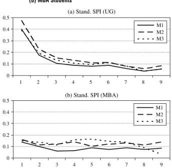
Our estimation analysis so far has focused on the mean effect of the influence of teams’ gender composition on SPI. However, it is also important to understand how the effect of the team’s gender com-position on SPI varies at different points of the per-formance distribution. In order to do so, we estimate quantile regressions using Equation (1). The results are shown in Figures 1(a) and 1(b), where we plot the coefficients for the different gender compositions, M1, M2, and M3, relative to the omitted category, M0, for each quantile, for undergraduates and MBA students, respectively. Thus the distance between the coefficients, with respect to the horizontal axis, reflects the distance with respect to M0 teams. Table 5 reports the point estimates for the 10th, 20th, 50th, 80th, and 90th quantiles.
We start by analyzing the undergraduate case. Fig-ure 1(a) and panel A of Table 5 show that M0 teams are significantly dominated by teams with any other gender combination throughout the entire perfor-mance distribution. Interestingly, we see large dispar-ities in the magnitudes of these effects. Most notably, the largest differences come from the bottom of the performance distribution, and they decrease mono-tonically along the distribution. Whereas for teams whose performance is at the bottom 10% of the distri-bution, the M0 teams are outperformed by 0.40, 0.47, and 0.39 of a standard deviation of the mean by M1, M2, and M3 teams, respectively, for teams whose per-formance is at the top 10% of the distribution, the M0 teams are outperformed by less than 0.09 of a stan-dard deviation.
12We also consider a different way of controlling for the team’s
field of study. We construct dummy variables that identify every possible combination of different fields of study; e.g., EBS is a dummy variable that takes the value of 1 when the team is com-posed of an economics student, a business student, and a science student and 0 otherwise. The results are both qualitatively and quantitatively the same.
Figure 1 Distributional Analysis for (a) Undergraduates and (b) MBA Students
(a) Stand. SPI (UG)
0 0.1 0.2 0.3 0.4 0.5 1 2 3 4 5 6 7 8 9 M1 M2 M3
(b) Stand. SPI (MBA)
0 0.1 0.2 0.3 0.4 0.5 1 2 3 4 5 6 7 8 9 M1 M2 M3
Notes. 10% to 90% quantile. Table 5 reports the coefficients for the 10%, 20%, 50%, 80%, and 90% levels, and includes the significance levels. All quantiles control for observable characteristics (as listed in Table 4) as well as control for year and zone fixed effects. The standard errors in all columns are clustered at the year and zone level. The dependent variable, SPI, is stan-dardized to a distribution with zero mean and a unit standard deviation for all quantiles. The team gender categories, M1, M2, and M3, are all compared with the excluded category, M0.
These results are informative for three reasons. First, we see that the underperformance of three-women teams is persistent throughout the entire distribution. Second, there is a great deal of hetero-geneity in the disparity. In particular, it is important to stress that the high performing three-women teams are much more similar to teams of any other gen-der combination. Third, the point estimates suggest that the mixed team, composed of two men and one woman, has the highest performance levels all over the distribution. This is in line with our findings in §4.1, when studying the overall effect. However, these differences are not significant at conventional levels, so they provide only suggestive evidence.
Figure 1(b) and panel B in Table 5 report the results for the MBA students. The coefficients for all the gender combinations, with respect to M0, are positive along the entire distribution, suggesting that three-women teams are underperforming. Inter-estingly, unlike the undergraduates, the differences are less robust across the distribution and are often insignificant, especially in the bottom half of the dis-tribution. Furthermore, at the top 10 percentile, we see that the only gender composition performing sig-nificantly better than M0 teams is the team composed of two men and one woman. This again provides evi-dence in favor of gender diversity at the top of the performance distribution.
Table 5 Gender Composition of Teams on SPI: Distributional Analysis
Panel A: Undergraduates Panel B: MBA students
Stand. SPI Stand. SPI Stand. SPI Stand. SPI Stand. SPI Stand. SPI Stand. SPI Stand. SPI Stand. SPI Stand. SPI
10% 20% 50% 80% 90% 10% 20% 50% 80% 90% Quantiles (1) (2) (3) (4) (5) (1) (2) (3) (4) (5) M1 00400∗∗∗ 00175∗∗∗ 000797∗∗∗ 000375∗ 000580∗∗∗ 00138 00065 000889∗∗ 000727 000441 60008857 60004317 60002937 60002237 60002137 6001197 60006137 60004207 60004817 60007117 M2 00476∗∗∗ 00224∗∗∗ 00108∗∗∗ 000614∗∗∗ 000859∗∗∗ 0016 00141∗∗ 00103∗∗ 00113∗∗ 00138∗∗ 60008877 60004297 60002917 60002217 60002127 6001157 60005917 60004057 60004657 60006817 M3 00392∗∗∗ 00189∗∗∗ 000938∗∗∗ 000383 000555∗∗ 00149 00159∗∗∗ 00164∗∗∗ 000871∗ 000314 60009207 60004477 60003067 60002337 60002197 6001187 60006017 60004117 60004687 60006817 Constant −20114∗∗∗ −00728∗∗∗ −0024 00420∗∗∗ 00963∗∗∗ −20207∗∗∗ −00681∗∗∗ −00231 00528∗∗∗ 00924∗∗∗ 6005947 6002797 6001837 6001357 6001297 6004767 6002467 6001707 6001917 6002627
Controls Yes Yes Yes Yes Yes Yes Yes Yes Yes Yes
Year FE Yes Yes Yes Yes Yes Yes Yes Yes Yes Yes
Zone FE Yes Yes Yes Yes Yes Yes Yes Yes Yes Yes
Cluster Yes Yes Yes Yes Yes Yes Yes Yes Yes Yes
Observations 8,997 8,997 8,997 8,997 8,997 3,481 3,481 3,481 3,481 3,481
Notes. The standard errors in all columns are clustered at the year and zone level. The dependent variable, SPI, is standardized to a distribution with zero mean and a unit standard deviation. The excluded team gender category is M0 (i.e., all-women teams). This table corresponds to Figures 1(a) and 1(b).
∗,∗∗, and∗∗∗denote significance at the 10%, 5%, and 1% levels, respectively.
5.
Understanding the Differences in
Performance: The Decision
Analysis
We have shown that all-women teams are signifi-cantly outperformed by teams with any other gender composition. In this section, we proceed to under-stand these differences in performance by analyzing the managerial decisions that teams undertake. In particular, we study team decision making on R&D, brand management, and social and environmental responsibility initiatives. In the analysis that follows, we estimate Equation (1) for each of the three decision variables, including all the controls as in columns (3) and (4) in Table 4.
5.1. Investments in R&D
We analyze whether teams with different gender compositions make significantly different decisions regarding the number of formulae to develop and the investment in R&D. The results are shown in Table 6. Columns (1) and (2) in Table 6 show the estimates for the number of formulae. Both at the undergraduate and MBA levels, all gender combinations have signif-icantly more formulae than do M0 teams. Columns (3) and (4) in Table 6 show the estimates for the stan-dardized R&D investment. Because there are signifi-cant differences in the developed number of formulae, we look at the R&D investment controlling for the number of formulae. The results in the table show that all teams invest more in R&D than do the three-women teams, even after controlling for the number of formulae.
Given these results, we conclude that the underper-formance of three-women teams is, in part, explained by their behavior related to R&D; that is, women teams invest too little in R&D (see Tables 1 and 2). A possible interpretation of these differences is that all-women teams are more risk averse in their man-agement vision. That is, all-women teams seem to Table 6 Gender Composition of Teams on R&D Decisions
Number of formulae Stand. R&D investment UG MBA students UG MBA students
(1) (2) (3) (4) M1 000350∗∗ 000669∗ 000738∗∗∗ 00142∗∗ 60001567 60003317 60002367 60005317 M2 000510∗∗ 000600∗∗ 00118∗∗∗ 00196∗∗∗ 60001997 60002367 60002637 60005857 M3 000533∗∗∗ 000651∗∗ 000809∗∗ 00199∗∗∗ 60001877 60002757 60003887 60004897 Number of 00902∗∗∗ 00863∗∗∗ formulae 60003447 60004367 Constant 10212∗∗∗ 10139∗∗∗ −10702∗∗∗ −10949∗∗∗ 60009337 60010007 6001597 6002347
Controls Yes Yes Yes Yes
Year FE Yes Yes Yes Yes
Zone FE Yes Yes Yes Yes
Cluster Yes Yes Yes Yes
Observations 7,561 2,910 7,561 2,910
Notes. The standard errors in all columns are clustered at the year and zone level. The dependent variable,R&D investment, in columns (3) and (4), is standardized to a distribution with zero mean and a unit standard deviation. The excluded team gender category is M0 (i.e., all-women teams).
∗, ∗∗, and ∗∗∗ denote significance at the 10%, 5%, and 1% levels,
Figure 2 Variation in SPI Conditional on R&D Investment 1 80 85 90 95 100 105 SPI 110 2 3 4 R&D investment
Notes. The first bin of the bar chart corresponds to R&D investment less than 1,000,000; the second bin corresponds to R&D investment between 1,000,000 and 2,500,000; the third bin corresponds to R&D investment between 2,500,000 and 5,000,000; and the fourth bin corresponds to R&D investment more than 5,000,000.
overweight the cost associated to R&D decisions with respect to the potential improvement in the ultimate value of the firm. Indeed, R&D decisions can be inter-preted as risky decisions. Looking at the variance of performance conditional in R&D investment, we see that as investment in R&D increases, the variance produced in performance increases significantly, sug-gesting riskier choice (see Figure 2).13
The literature on gender differences at the indi-vidual level has consistently documented differences in risk preferences, that women tend to be more risk-averse than men (see Eckel and Grossman 2003, Croson and Gneezy 2009). In this sense, all-women teams being more risk averse is in line with the find-ings at the individual level. Interestingly, we also see that mixed teams are not significantly different from all-men teams, such that having one man or three men does not show significant differences in the team’s R&D investment.
5.2. Brand Management
We now analyze the impact of teams’ gender com-position on the midway outcome variables that are directly determined by brand management. We start with an analysis at the aggregate level, looking at (standardized) variables such as profits, revenues, costs, sales, and inventories. We then break down the aggregate analysis to study each of the brands separately.
The main outcome variable related to brands is profits. Accordingly, we first analyze whether the level of total profits earned by teams varies across the different gender compositions. In columns (1) and (2) of Table 7, we report the profits at the aggre-gate level separately for undergraduates and MBA
13Looking at the mean investment by team gender composition,
the mean investment by M0 teams is in the second bin of Figure 2, whereas all other teams’ investments are in the third bin.
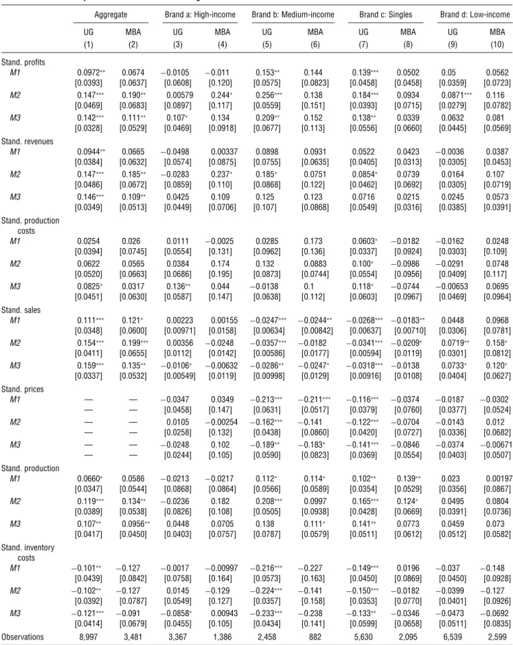
students. Both at the undergraduate and MBA lev-els, we find that every gender composition achieves significantly higher profits than do M0 teams. When we separate the profits into revenues and production costs, we see that the difference is largely related to differences in revenues but not in production costs. The M1, M2, and M3 teams attain significantly higher revenues than do M0 teams, but there are no signif-icant differences in production costs. Consistent with these results, Table 7 also shows that all teams pro-duce more than the M0 teams, but they also sell more, resulting in lower inventory costs. These differences highlight that the underperformance of M0 teams is also related to their brand management. We see that M0 teams are choosing worse selling strategies than are the rest of teams.
To understand the differences in their selling strat-egy, we now turn our attention to the analysis of brand management at the brand-type level. Con-sumers are divided into five different segments, which differ in size, price sensitivity, and prefer-ences. Teams are provided with this information in their instruction manuals. The five segments, ordered by their income (highest to lowest) and price sen-sitivity (lowest to highest), are (i) high earners, (ii) affluent families, (iii) medium-income families, (iv) singles, and (v) low-income families. Accordingly, brands differ in terms of the type of consumers to which they are targeted. In the three editions of the game in our database, there were four different brand types: (a) high income (edition 2007), (b) medium-income families (2009), (c) singles (2008 and 2009), and (d) low income (2007 and 2008).
Columns (3)–(10) in Table 7 report the analysis at the brand-type level. We see that for undergraduates, the differences identified at the aggregate level, in terms of profits, revenues, sales, and inventory costs, are concurrent only for brand types (b) and (c); the intermediate brand types. When we analyze the other brands, the high-income and low-income brand types, there is almost no difference across teams. We next consider the differences in teams’ pricing strategies. We see that with brand types (b) and (c) that M0 teams choose significantly higher prices than do all other gender composition teams. This pricing strat-egy results in significantly lower revenues (and prof-its) for the M0 teams; in turn, this also explains why M0 teams have significantly higher inventory costs. We can interpret such a pricing strategy by M0 teams as being less aggressive than the rest of the teams’. Again, the literature on gender differences at the indi-vidual level offers a plausible explanation for these findings. In particular, it has been shown that women and men have different attitudes toward competi-tion. Not only do women seem to dislike competition
Table 7 Gender Composition of Teams on Brand Management
Aggregate Brand a: High-income Brand b: Medium-income Brand c: Singles Brand d: Low-income
UG MBA UG MBA UG MBA UG MBA UG MBA
(1) (2) (3) (4) (5) (6) (7) (8) (9) (10) Stand. profits M1 000972∗∗ 000674 −000105 −00011 00153∗∗ 00144 00139∗∗∗ 000502 0005 000562 60003937 60006377 60006087 6001207 60005757 60008237 60004587 60004587 60003597 60007237 M2 00147∗∗∗ 00190∗∗ 0000579 00244∗ 00256∗∗∗ 00138 00184∗∗∗ 000934 000871∗∗∗ 00116 60004697 60006837 60008977 6001177 60005597 6001517 60003937 60007157 60002797 60007827 M3 00142∗∗∗ 00111∗∗ 00107∗ 00134 00209∗∗ 00152 00138∗∗ 000339 000632 00081 60003287 60005297 60004697 60009187 60006777 6001137 60005567 60006607 60004457 60005697 Stand. revenues M1 000944∗∗ 000665 −000498 0000337 000898 000931 000522 000423 −000036 000387 60003847 60006327 60005747 60008757 60007557 60006357 60004057 60003137 60003057 60004537 M2 00147∗∗∗ 00185∗∗ −000283 00237∗ 00185∗ 000751 000854∗ 000739 000164 00107 60004867 60006727 60008597 6001107 60008687 6001227 60004627 60006927 60003057 60007197 M3 00146∗∗∗ 00109∗∗ 000425 00109 00125 00123 000716 000215 000245 000573 60003497 60005137 60004497 60007067 6001077 60008687 60005497 60003167 60003857 60003917 Stand. production costs M1 000254 00026 000111 −000025 000285 00173 000603∗ −000182 −000162 000248 60003947 60007457 60005547 6001317 60009627 6001367 60003377 60009247 60003037 6001097 M2 000622 000565 000384 00174 00132 000883 00100∗ −000986 −000291 000748 60005207 60006637 60006867 6001957 60008737 60007447 60005547 60009567 60004097 6001177 M3 000825∗ 000317 00136∗∗ 00044 −000138 001 00118∗ −000744 −0000653 000695 60004517 60006307 60005877 6001477 60006387 6001127 60006037 60009677 60004697 60009647 Stand. sales M1 00111∗∗∗ 00121∗ 0000223 0000155 −000247∗∗∗ −000244∗∗ −000268∗∗∗ −000183∗∗ 000448 000968 60003487 60006007 600009717 60001587 600006347 600008427 600006377 600007107 60003067 60007817 M2 00154∗∗∗ 00199∗∗∗ 0000356 −000248 −000357∗∗∗ −000182 −000341∗∗∗ −000209∗ 000719∗∗ 00158∗ 60004117 60006557 60001127 60001427 600005867 60001777 600005947 60001197 60003017 60008127 M3 00159∗∗∗ 00135∗∗ −000106∗ −0000632 −000286∗∗ −000247∗ −000318∗∗∗ −000138 000733∗ 00120∗ 60003377 60005327 600005497 60001197 600009987 60001297 600009167 60001087 60004047 60006277 Stand. prices M1 — — −000347 000349 −00213∗∗∗ −00211∗∗∗ −00116∗∗∗ −000374 −000187 −000302 — — 60004587 6001477 60006317 60005177 60003797 60007607 60003777 60005247 M2 — — 000105 −0000254 −00162∗∗∗ −00141 −00122∗∗∗ −000704 −000143 00012 — — 60002587 6001327 60004387 60008607 60004207 60007277 60003367 60006827 M3 — — −000248 00102 −00189∗∗ −00183∗ −00141∗∗∗ −000846 −000374 −0000671 — — 60002447 6001057 60005907 60008237 60003697 60005547 60004037 60005077 Stand. production M1 000660∗ 000586 −000213 −000217 00112∗ 00114∗ 00102∗∗ 00139∗∗ 00023 0000197 60003477 60005447 60008687 60008647 60005667 60005897 60003547 60005297 60003567 60008677 M2 00119∗∗∗ 00134∗∗ −000236 00182 00208∗∗∗ 000997 00165∗∗∗ 00124∗ 000495 000804 60003897 60005387 60008267 6001087 60005057 60009387 60004287 60006697 60003917 60007367 M3 00107∗∗ 000956∗∗ 000448 000705 00138 00111∗ 00141∗∗ 000773 000459 00073 60004177 60004507 60004037 60007577 60007877 60005797 60005117 60006127 60005127 60005827 Stand. inventory costs M1 −00101∗∗ −00127 −000017 −0000997 −00216∗∗∗ −00227 −00149∗∗∗ 000196 −00037 −00148 60004397 60008427 60007587 6001647 60005737 6001637 60004507 60008697 60004507 60009287 M2 −00102∗∗ −00127 000145 −00129 −00224∗∗∗ −00141 −00150∗∗∗ −000182 −000399 −00127 60003927 60007877 60005497 6001277 60003577 6001587 60003537 60007707 60004017 60009267 M3 −00121∗∗∗ −00091 −000858∗ 0000943 −00233∗∗∗ −00238 −00133∗∗ −000346 −000473 −000692 60004147 60006797 60004557 6001057 60004347 6001417 60005997 60006587 60005117 60008357 Observations 8,997 3,481 3,367 1,386 2,458 882 5,630 2,095 6,539 2,599
Notes. All columns control for observable characteristics as in columns (3) and (4) in Table 4, as well as controls for year and zone fixed effects. The standard errors in all columns are clustered at the year and zone level. The dependent variables in all columns are standardized to a distribution with zero mean and a unit standard deviation. The excluded team gender category is M0 (i.e., all-women teams).
Table 8 Gender Composition of Teams on Corporate Responsibility Stand. SSI Stand. ESI
UG MBA UG MBA (1) (2) (3) (4) M1 −000708∗∗ −000900∗ 000202 −000181 60003297 60004507 60002597 60009537 M2 −00126∗∗∗ −000701 000261 000135 60003457 60005337 60003157 60006807 M3 −000888∗∗ −00160∗∗∗ −000216 −000306 60003817 60004877 60003357 60007367 Constant 0033 00696∗∗∗ −000649 −00207 6002047 6002187 6002117 6002717
Controls Yes Yes Yes Yes
Year FE Yes Yes Yes Yes
Zone FE Yes Yes Yes Yes
Cluster Yes Yes Yes Yes
Observations 8,855 3,405 8,855 3,405
Notes. The standard errors in all columns are clustered at the year and zone level. The dependent variables in all columns are standardized to a distribu-tion with zero mean and a unit standard deviadistribu-tion. The excluded team gender category is M0 (i.e., all-women teams).
∗, ∗∗, and ∗∗∗ denote significance at the 10%, 5%, and 1% levels,
respectively.
more than men do, but under competition the perfor-mance of men is improved relative to that of women (see Gneezy et al. 2003, Gneezy and Rustichini 2004, Niederle and Vesterlund 2007).14Arguably, setting the
price is a form of competition, and hence that M0 teams are not competitive enough can be related to the findings above.
The analysis at the MBA level, when disaggregated by brand types, does not show consistent and clear significant differences. This is likely to be the result of a reduction in the number of observations, and hence the significance levels are lower. However, the magni-tudes and signs are comparable to those found at the aggregate level.
5.3. Corporate Responsibility
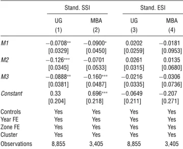
We now study whether the gender composition of the team has any effect on the social and environ-mental responsibility decisions, as measured by the standardized SSI and ESI indices. Table 8 reports the results. With regard to social initiatives, we find that three-women teams invest significantly more in social initiatives than does any other gender composition, both at the undergraduate and MBA level. These dif-ferences are as large as 0.12 and 0.16 of a standard deviation from the mean in undergraduate and MBA competitions, respectively. All comparisons are signif-icant, except in the M2 case for MBA students where
14When team performance is defined as the sum of two
individ-uals’ independent performance, it has been shown that gender differences under competition are reduced (see Dargnies 2010, Healy and Pate 2011).
the coefficient goes in the same direction than all oth-ers, but it is not significant at conventional levels. In columns (3) and (4), on the other hand, the gender composition of the teams does not appear to influence decisions related to environmental initiatives.
Hence, gender composition seems to matter for the type of decisions taken regarding social initiatives. In §2.3 we observed that SSI is positively related to SPI. However, we also observed that the influence on SPI of the social sustainability initiatives is of an order of magnitude lower than is profits. This shows that although M0 teams invest significantly more in SSI, it has little impact on the final and main outcome vari-able, on SPI. From Table 1, the polynomial regressions show that there are diminishing returns to spending on SSI, which suggests that M0 may be overinvesting in SSI.
The literature on gender differences at the individ-ual level provides mixed evidence on differences with regard to altruism, values, and social preferences (see Croson and Gneezy 2009). Although there are papers reporting that women are significantly more altruistic than men are (see Eckel and Grossman 1998, Bolton and Katok 1995, Andreoni and Vesterlund 2001) and that women have more social oriented values than men have (see Adams and Funk 2011), other papers also show that the behavior of women in social con-texts is highly sensitive to the details of the context (see Ben-Ner et al. 2004, Houser and Schunk 2009). Our findings related to corporate responsibility deci-sions of teams seem to be mixed, in line with the literature. In particular, whereas in the case of social initiatives all-women teams invest significantly more than do all other teams, in the case of environmental initiatives there are no significant differences.
6.
Discussion
We have shown that three-women teams are out-performed by teams of any other gender combina-tion and that there is not a monotonic relacombina-tionship between the number of men and team performance. Because teams are formed endogenously, there are competing explanations for our findings. It is impor-tant to discuss these explanations because the policy, social, and scientific conclusions one could draw from our results are clearly very different depending on what drives them.
We distinguish between two broad competing explanations. First, participating women and men may be different in terms of their unobservable char-acteristics, such as ability, expectations about the reward structure implicit in the game, or the way in which they sort into teams. Second, three-women teams may have worse team dynamics than do teams of any other gender composition, such that, despite