WO R K I N G PA P E R S E R I E S
N O. 5 2 9 / S E P T E M B E R 2 0 0 5
EXPLAINING EXCHANGE
RATE DYNAMICS
THE UNCOVERED
EQUITY RETURN PARITY
CONDITION
by Lorenzo Cappiello
and Roberto A. De Santis
In 2005 all ECB publications will feature a motif taken from the €50 banknote.
W O R K I N G PA P E R S E R I E S
N O. 5 2 9 / S E P T E M B E R 2 0 0 5
This paper can be downloaded without charge from http://www.ecb.int or from the Social Science Research Network electronic library at http://ssrn.com/abstract_id=804924.
EXPLAINING EXCHANGE
RATE DYNAMICS
THE UNCOVERED
EQUITY RETURN PARITY
CONDITION
1by Lorenzo Cappiello
2and Roberto A. De Santis
31 We are indebted to Olivier Blanchard, Giancarlo Corsetti, Luca Dedola, Kenneth Froot, Bruno Gerard, Philipp Hartmann, Robert Lucas, Simone Manganelli, Andrew Rose, Chiara Osbat, Bernd Schnatz and seminar participants at the 2005 Econometric Society World Congress (London) for their valuable comments
© European Central Bank, 2005
Address Kaiserstrasse 29
60311 Frankfurt am Main, Germany
Postal address Postfach 16 03 19
60066 Frankfurt am Main, Germany
Telephone +49 69 1344 0 Internet http://www.ecb.int Fax +49 69 1344 6000 Telex 411 144 ecb d
All rights reserved.
Any reproduction, publication and reprint in the form of a different publication, whether printed or produced electronically, in whole or in part, is permitted only with the explicit written authorisation of the ECB or the author(s).
The views expressed in this paper do not necessarily reflect those of the European Central Bank.
The statement of purpose for the ECB Working Paper Series is available from the ECB website, http://www.ecb.int.
ISSN 1561-0810 (print) ISSN 1725-2806 (online)
C O N T E N T S
Abstract 4
Non-technical summary 5
1 Introduction 7
2 The uncovered equity return parity condition 9
3 Testing the uncovered equity return parity
condition 10
4 Data 13
5 Empirical results 15
6 Can we beat the random walk? 17
7 Summary of results and conclusions 20
References 22
Appendix 24
Figures and tables 28
Abstract
By employing Lucas’ (1982) model, this study proposes an arbitrage relationship – the Uncovered Equity Return Parity (URP) condition – to explain the dynamics of exchange rates. When expected equity returns in a country/region are lower than expected equity returns in another country/region, the currency associated with the market offering lower returns is expected to appreciate. First, we test the URP assuming that investors are risk neutral and next we relax this hypothesis. The resulting risk premia are proxied by economic variables, which are related to the business cycle. We employ differentials in corporate earnings’ growth rates, short-term interest rate changes, annual inflation rates, and net equity flows. The URP explains a large fraction of the variability of some European currencies vis-à-vis the US dollar. When confronted with the naïve random walk model, the URP for the EUR/USD performs better in terms of forecasts for a set of alternative statistics.
JEL Classification: F31, G15, C22, C53
Keywords: foreign exchange markets; asset pricing; random walk; UIP; GMM
Non-technical summary
The need to understand the mechanics of exchange rates and their developments has generated a vast theoretical and empirical literature. The flexible price monetary model, which subsequently gave way to the overshooting or sticky-price model, the equilibrium and liquidity models as well as the portfolio balance approach have characterised three decades of research, from the 1960s to the 1980s. More recently, since the publication of Obstfeld and Rogoff’s (1995) seminal “redux” paper, the new open-economy macroeconomics has attempted to explain exchange rate developments in the context of dynamic general equilibrium models that incorporate imperfect competition and nominal rigidities. Empirically, these theoretical developments have fared poorly at explaining exchange rate dynamics, at least over relatively short horizons, and several exchange rate puzzles have been highlighted.
The increasing role played by international financial markets in developed economies constitutes a persuasive argument to explore possible relationships between returns on risky assets and exchange rates dynamics. Recently, a new strand of research has investigated the interconnections between equity and bond returns, on one side, and exchange rate dynamics, on the other side, with promising results (see Brandt et al., 2001; Pavlova and Rigobon, 2003; Hau and Rey, 2004 and 2005).
In this paper, by employing the Lucas’ (1982) consumption economy model, we introduce a new framework explaining exchange rate dynamics. We propose an arbitrage relationship between expected exchange rate changes and differentials in expected equity returns of two economies. Specifically, if expected returns on a certain equity market are higher than those obtainable from another market, the currency associated with the market that offers higher returns is expected to depreciate. A resident in the market which offers higher expected returns suffers a loss when investing abroad, and therefore she has to be compensated by the expected capital gain that occurs when the foreign currency appreciates. This ensures that no sure opportunities for unbounded profits exist and, therefore, the equilibrium is re-established. Due to the similarity with the Uncovered Interest Parity (UIP) condition, the equilibrium hypothesis proposed and tested here is baptised Uncovered Equity Return Parity condition (URP). There is, however, a key difference between the two arbitrage relations. In the UIP return differentials are known ex ante, since they are computed on risk-free assets, while in the URP are not.
Risk-averse agents investing in risky assets denominated in a foreign currency usually require a market and a foreign exchange risk premium, which can be time varying. We begin our study assuming that investors are risk-neutral, which implies that the URP does not include risk
premia. Next, we relax the risk-neutrality assumption and we enrich the URP by employing additional financial variables, which are related to the business cycle. We use differentials in corporate earnings’ growth rates, short-term interest rate changes, and annual inflation rates, as well as net equity flows. In line with previous studies (see, for instance, Fama and French, 1989; Chen, 1991; and Ferson and Harvey, 1991b), these variables can be thought of as proxies for the risk premia. The URP with risk premia turns out to explain a large fraction of the variability of the European currencies, particularly of the euro, the British pound and the Swiss franc.
We also test the forecasting ability of the URP with time-varying risk premia and find that it beats the naïve random walk model with drift at two- and three-month ahead forecasts and always predicts about two thirds of directional changes for the EUR/USD exchange rate. The forecasting performances for the Swiss Franc are better in terms of mean square errors, but not in terms of the sign tests. The specification for the British pound does not beat the naïve random walk model, despite it predicts correctly more than 60% of its directional changes.
Similar specifications fail in explaining the evolution of the Japanese Yen and the Canadian dollar against the US dollar, possibly due to the systematic intervention policy of these countries in the foreign exchange market.
"My experience is that exchange markets have become so efficient that virtually all relevant information is embedded almost instantaneously in exchange rates to the point that anticipating movements in major currencies is rarely possible….. To my knowledge, no model projecting directional movements in exchange rates is significantly superior to tossing a coin."
FED Chairman Alan Greenspan, at the 21st Annual Monetary Conference, Washington, D.C., November 20, 2003.
1.
Introduction
The need to understand the mechanics of exchange rates and their developments has generated a vast theoretical and empirical literature.1 The flexible price monetary model, which subsequently gave way to the overshooting or sticky-price model, the equilibrium and liquidity models as well as the portfolio balance approach have characterised three decades of research, from the 1960s to the 1980s. More recently, since the publication of Obstfeld and Rogoff’s (1995) seminal “redux” paper, the new open-economy macroeconomics has attempted to explain exchange rate developments in the context of dynamic general equilibrium models that incorporate imperfect competition and nominal rigidities. Empirically, these theoretical developments have fared poorly at explaining exchange rate dynamics, at least over relatively short horizons, and several exchange rate puzzles have been highlighted.23
In this paper, by employing the Lucas’ (1982) consumption economy model, we introduce a new framework explaining exchange rate dynamics. We propose an arbitrage relationship between expected exchange rate changes and differentials in expected equity returns of two economies. Specifically, we show that when expected returns on a certain equity market are lower than the returns that could be gained from another market, the currency associated with the market that offers lower average returns is expected to appreciate. This ensures that no sure opportunities for unbounded profits exist and, therefore, the equilibrium is re-established. Due to the similarity with
1
Surveys can be found for instance in Hodrick (1987), Frankel and Rose (1995), Taylor (1995), Engel (1996) and Lyons (2001).
2
Progress has been recently made in the microstructure literature. Evans and Lyons (2002), for instance, explain above 60% of daily changes in log exchange rates, demonstrating that there is high correlation between net order flows from electronic brokerage systems and contemporaneous exchange rate changes. The downside of this research is that, ultimately, order flows do not reveal why investors approach a market-maker to execute their buy or sell orders, leaving exchange rate determinants quite obscure.
3
The two most well-known puzzles are: (i) the determination puzzle, which points out that exchange rate movements cannot be explained by macroeconomic fundamentals; and (ii) the forward rate puzzle (or Uncovered Interest Parity condition – UIP – puzzle), which highlights that the forward exchange rate is a biased predictor of the future spot rate, or, put it differently, that short-term interest rate differentials fail to explain changes in spot exchange rates.
the UIP, the equilibrium hypothesis proposed and tested here is baptised Uncovered Equity Return Parity condition (URP).
Several studies have recently analysed the interaction between risky asset returns and exchange rates. Brandt et al. (2001) argue that exchange rates fluctuate less than the implied marginal rate of intertemporal substitution obtained from equity market premia. Pavlova and Rigobon (2003) describe a two-country two-good asset pricing model, where the same factors drive real exchange rates, equity and bond markets. Estimates suggest that demand shocks are twice as important as output innovations in explaining the dynamics of exchange rates and asset prices. Hau and Rey (2004, 2005) put emphasis to the inter-connections between dynamic asset allocation and exchange rate evolution, developing a theoretical model where exchange rates, equity market returns and equity flows are jointly and endogenously determined. Imbalances between the domestic and foreign dividend income, which are generated by differences in stock market performances, determine dynamic re-balancing of equity portfolios, which, in turn, initiate foreign exchange order flows and therefore exchange rate movements.4
Similarly to our findings, one of the implications of the model developed by Hau and Rey (2005) is that “higher returns in the home equity market (in local currency) relative to the foreign equity market are associated with a home currency depreciation”. The relationship between equity and foreign exchange markets allows them to talk about “uncovered equity parity”. The key difference with Hau and Rey is that, in our framework, the imbalances between dividend incomes are not the driving forces of exchange rate developments. The model that we propose tests a simple arbitrage condition. The analysis is carried out on the euro, the Japanese yen, the Pound sterling, the Swiss franc, the Canadian dollar, the French franc and the Deutsche Marc vis-à-vis the US dollar.5 The results suggest that differentials in returns on equity prices exhibit explanatory power for the dynamics of all European currencies against the US dollar.
Risk-averse agents investing in risky assets denominated in a foreign currency usually require a market and a foreign exchange risk premium. As pointed out already by Fama (1984), risk premia can be time varying and linked to the business cycle. We begin our study assuming that investors
4
Additional studies linking risky assets to exchange rates have been developed by the international asset pricing literature. An example is the International Capital Asset Pricing Model (Solnik, 1974; Adler and Dumas, 1983), where risk averse international investors require a market premium to hedge against uncertain security returns, and an exchange rate risk premium to hedge against currency risks stemming from those assets denominated in foreign currency.
5
Although French franc and Deutsche mark ceased to exist with the advent of the euro in January 1999, results on these two currencies are reported for robustness check with the sample period ending in December 1998.
are neutral, which implies that the URP does not include risk premia. Next, we relax the risk-neutrality assumption and we enrich the URP by employing additional financial variables, which are related to the business cycle. We use differentials in corporate earnings’ growth rates, short-term interest rate changes, and annual inflation rates, as well as net equity flows. In line with previous studies (see, for instance, Fama and French, 1989; Chen, 1991; and Ferson and Harvey, 1991b), these variables can be thought of as proxies for the risk premia. The URP with risk premia turns out to explain a large fraction of the variability of the European currencies, particularly of the euro, the British pound and the Swiss franc.
A financial variable usually monitored by private and institutional investors is the equities’ earnings yield or the inverse of the price-earnings ratio, which indicates how much investors are willing to pay a stock per unit of earnings. As a complementary analysis to the URP, we investigate a relationship between exchange rates developments and growth rates of earnings yields across regions/countries. Indeed, the differentials in growth rates of earning yields, on the one hand, and the differentials in equity returns and growth rates of total earnings, on the other hand, are, under some mild assumptions, the two sides of the same coin. We find that the differential of earning yields’ growth rates is a key variable to explain movements in the exchange rate of the euro, the Pound sterling and the French franc vis-à-vis the US dollar, and that the results are consistent with the URP condition.
The remainder of the paper is organised as follows: Sections 2 and 3 present the URP hypothesis and the empirical models, respectively. Section 4 describes the data utilised in the analysis. Section 5 discusses the empirical results. Section 6 tests the robustness of the model through predictive accuracy as well as directional change tests. Section 7 concludes the paper. Finally, Appendix A formally derives the URP.
2.
The uncovered equity return parity condition
The equilibrium condition proposed in this paper relates the expected changes in exchange rates with differentials in the expected returns on equity securities. Exchange rates and equity returns would move simultaneously in order to guarantee equilibrium in international financial markets. The theoretical foundations of this arbitrage condition can be found in Lucas’ (1982) consumption economy. Lucas develops a dynamic, two country, general equilibrium model, thanks to which we derive the URP enriched with risk premia. In Lucas’ model the only risky assets traded are claims to countries’ uncertain outputs, or, put it differently, shares of stocks in national economies. While the asset pricing literature has utilised Lucas’ framework because it provides useful insights into the
nature of risk premia in asset markets, we extend Lucas’ model putting emphasis on the exchange rate dynamic as a function of differentials in expected returns on two regional equity markets.
Lucas’ model is sketched in Appendix A, where the URP is also formally derived. Specifically, we show that the dynamics between returns on risky assets and exchange rate among two countries are linked by the following expression:
(1)
{
(
)
}
{
(
)
}
1 , 1 , 1 , 1 , 1 1 + + + + + ⎪⎭ ⎪ ⎬ ⎫ ⎪⎩ ⎪ ⎨ ⎧ ℑ ℑ + = ℑ + t t t ij t ij t t y t t x riskpremium S S E R E R Ewhere E
{
(
1+Rx,t+1)
ℑt}
and E{
(
1+Ry,t+1)
ℑt}
are expected gross total returns resulting from producing goods x in country i and goods y in country j, given the information set ℑt; Sijt, is the nominal spot exchange rate of currency i with respect to currency j, that is the number of units of currency i exchanged for one unit of currency j (for instance euro per US dollars). Finally, the variableriskpremiumt+1 includes equity as well as foreign exchange risk premia.For a given value of the risk premium term, the URP states that discrepancies in expected equity returns are re-equilibrated through contemporaneous adjustments in expected exchange rates. Specifically, if expected returns on a certain equity market are higher than those obtainable from another market, the currency associated with the market that offers higher returns is expected to depreciate. A resident in the market which offers higher expected returns suffers a loss when investing abroad, and therefore she has to be compensated by the expected capital gain that occurs when the foreign currency appreciates. The arbitrage mechanism characterising the URP is therefore similar to the one driving the UIP. There is, however, a key difference between the two arbitrage relations. In the UIP return differentials are known ex ante, since they are computed on risk-free assets, while in the URP are not.
3.
Testing the uncovered equity return parity condition
To render the model described by (1) empirically tractable, we assume - for the time being - that agents are risk neutral. Taking logarithms of both sides of (1) yields: 6
(2) E
{
sij,t+1ℑt}
−sij,t =−E{
rj,t+1 −ri,t+1ℑt}
,
6
Notice that equation (2) is only an approximation because of Jensen’s inequality, which implies that
{
ht t}
E{
ln( )
ht t}
E
ln +1ℑ > +1 ℑ .
where sij,t+1 ≡ln
(
Sij,t+1)
, rit,+1≡ ln(
1+Rx,t+1)
and rj,t+1≡ ln(
1+Ry,t+1)
. Specifically, E{
ri,t+1ℑt}
and{
rjt t}
E ,+1ℑ are, respectively, the expected equity returns in country i and j given the information set
t
ℑ .7
Assume also that the vector process
{ }
yt Tt=1, yt ≡(
sij,t,rj,t,ri,t)
′ is stationary and Gaussian, which implies that the conditional expectations in (2) have linear, time invariant representations and that the conditional variances are constant. Thanks to this assumption, once the projection{
rj,t ri,t t}
E +1− +1ℑ is parameterized as a linear function of some predetermined variables, the parameters of (2) can be estimated by the Generalized Method of Moments (GMM) of Hansen (1982). Although developments in exchange rate changes might be determined by equity return differentials, investors may well exploit profit possibilities arising from the foreign exchange markets. For example, if euro area investors expected a decline in the US dollar, they would demand higher returns on US assets to compensate for the expected loss. This would induce a portfolio re-balance, which in turn would impact stock returns. This simultaneity problem justifies the use of GMM.
The econometric relationship for the conditional expectation of equity return differential reads as follows:
(3) rj,t+1−ri,t+1 =δ′
(
Zj,t −Zi,t)
+ut+1,where Zj,t and Zit, are
(
f ×1)
vectors of instrumental variables, δ is a(
f ×1)
vector of coefficients and ut+1 represents the forecast error which is orthogonal to the information variables.The GMM procedure permits to estimate the following model: (4) ∆sijt,+1=γ+α
(
rjt,+1−rit,+1)
+εt+1,where the f orthogonality conditions are given by E
{
(
Zj,t −Zi,t)
εt+1}
=0. The Newey-West covariance estimator is employed and is consistent in the presence of heteroskedasticity and autocorrelation of unknown form (Newey and West, 1987).Under the hypothesis of market efficiency and risk neutrality, γ should not be statistically different from zero, while α should be equal to minus one. This would be in line with what the URP predicts to arbitrage away any profit possibilities. However, in the spirit of Fama’s (1984) argument about the forward rate puzzle, if investors are risk averse, α could be negative but
7
Since in Lucas (1982) Rx,t+1 and Ry,t+1 are the returns resulting from producing gods x and y, respectively, for
smaller than one in absolute value. The resulting risk premium could be time varying and affected by the business cycle. In line with earlier studies (Fama and French, 1989; Chen, 1991; Ferson and Harvey, 1991b), we assume that the risk premium is a function of a set of macroeconomic variables, such as the corporate earnings’ growth rates, international equity flows, the annual inflation rates, and the changes in the short-term interest rates. In a two country/region context, we consider differentials in the two regional risk premia, which, in turn, are associated with differentials of country-specific economic variables. Since these variables are related to regional business cycles, their associated coefficients also possess economic content. Therefore, the model described by equation (4) can be extended and take the following specification:
(5)
(
(
)
)
(
(
)
)
(
)
. 1 7 1 1 6 1 1 5 1 4 1 1 2 3 1 1 2 1 1 1 0 1 + + + + + + + + + + + + + ζ + ∆ α + − ∆ α + π − π ∆ α + α + − ∆ α + − ∆ α + − α + α = ∆ t t, ij t, i t, j t, i t, j t, ij t, i t, j t, i t, j t, i t, j t, ij s i i Q e e e e r r s 1 +∆ei,t
(
∆ej,t+1)
denotes the change in the log current corporate earnings associated with theequity price index i (j), which can approximate business cycle developments due to the pro-cyclical nature of corporate profits. When the growth rate of corporate earnings is relatively higher in one country/region, then its associated currency should appreciate vis-à-vis the other. Therefore, α2 is
expected to be positive. The change in the earnings growth differential, ∆2
(
ej,t+1−ei,t+1)
, determines whether that differential is itself increasing or decreasing. If, for example, a positive widening in the differential induced a further appreciation of currency j vis-à-vis currency i, the pattern of the exchange rate sij,t+1 would be unsustainable. Therefore the coefficient α3 is expected to be negative.1 ,t+ ij
Q represents the net equity flows from country/region i to j, which can also approximate business cycle developments. Since a positive (negative) change in net equity flows from country/region i to j could generate appreciation (depreciation) of the currency j vis-à-vis the currency i, α4 is expected to be positive. The inclusion of such variables could be criticized on the
ground of an indeterminacy issue: if equity flows may have an impact on exchange rate developments, it is also true that exchange rate movements, in turn, may affect capital flow directions. However, this is the case only if there is a temporal lag between the two variables. If
1
+
∆sij,t were regressed on ∆Qt, when investors decide in which market to allocate their funds, they would form expectations on possible evolutions of exchange rates. However, in equation (5), only a contemporaneous relationship between these two variables is explored.
(
,+1− ,+1)
∆ijt iit and ∆
(
πj,t+1−πi,t+1)
are the changes in differentials of the three-month interestrates and annual inflation rates, respectively. Both variables are key components of the business
cycle literature. The differential in the changes of short-term interest rates is a variable which is borrowed from the microstructure literature (see, for instance, Evans and Lyons, 2001), which adopts it in the spirit of the Dornbush’s (1976) model. More specifically, an increase in ∆ij,t+1 relative to ∆ii,t+1 should determine an appreciation of sij,t+1 (i.e. α6 >0). Investors monitor the
monthly changes in annual inflation rates, as inflation can undermine the purchasing power of their investments. If changes in inflation rates are higher in country j relative to country i, sij,t+1 is
expected to depreciate (i.e. α5 <0).
Finally, the term ∆sij,t captures a possible autoregressive component in the dependent variable.
We will also carry out a test to check whether the coefficients α1 and α2 are statistically the same, but of opposite sign, i.e. if α1 =−α2 =α. If this were the case and if the rate of growth of the
number of shares in each equity price index were relatively small or highly correlated, the term
(
1 1)
2(
1 1)
1 + − + +α ∆ + − +
α rjt, rit, ejt, eit, would be approximately equal to the change in the price-earnings ratio, i.e. α
{
∆ln(
Pj,t+1 Ej,t+1)
−∆ln(
Pi,t+1 Ei,t+1)
}
, where Ei,t+1(
Ej,t+1)
is the level of earnings per share for the equity price index Pi,t+1( )
Pj,t+1 . International investors usually shift their funds to purchase securities characterized by relatively better yields’ perspectives. In the equity markets, the price-earnings ratio is often used as a barometer of stocks’ evaluation, which helps recognize profitable investment opportunities. A stock’s price-earnings ratio indicates investors how much they are willing to pay per unit of earnings per share. Its inverse, the earnings yield, gives investors a reliable picture of a company management’s ability to make profits out of the amount invested in equities. Consequently, when making their portfolio choices, international investors could take into consideration relative growth in the earnings yield. Funds would be shifted where perspectives on earnings yields are relatively more attractive. Equivalently, given a certain amount of earnings in two different countries/regions, investors move capital where prices are lower. In this case, an increase (decrease) in earnings yields in country j, eyjt,+1, relative to country i, eyi,t+1, would bematched with an appreciation (depreciation) of currency j relative to i.
4.
Data
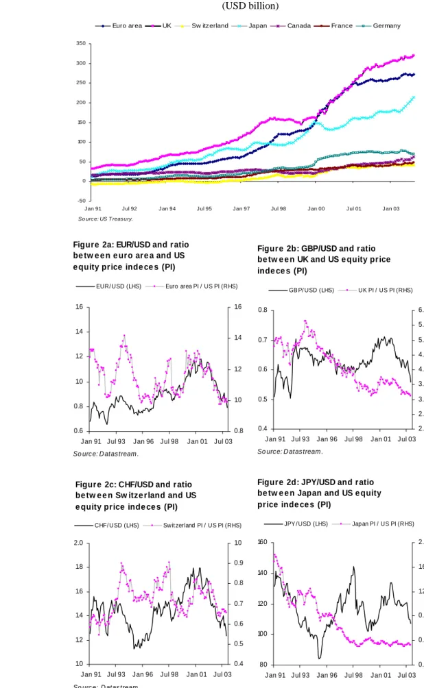
The empirical study is carried out using data from January 1991 to December 2003. The choice of this sample period is motivated by the large increase in cross-border equity flows due to financial liberalization of equity markets across the world. International equity flows on both the asset and
liability sides of the United States vis-à-vis all countries/regions investigated in this study skyrocketed over the 1990’s (see Figure 1).
All time series are observed at monthly frequency and obtained from Thomson Datastream. When financial variables are used, we employ the last trading day of the month.
Spot exchange rates include the synthetic euro until December 1998 and thereafter the actual euro (EUR), the Japanese Yen (JPY), the pound sterling (GBP), the Swiss franc (CHF), the Canadian dollar (CAD), the French franc (FF) and the Deutsche mark (DM), all against the US dollar (USD).8
Returns on equity securities are continuously compounded and computed with Thomson Datastream price indices for the United States, the euro area, Japan, the United Kingdom, Switzerland, Canada, France and Germany. Returns do not include dividends, since dividend yields will be employed as instruments and growth rates of earnings will enter the analysis as a separate regression variable. Datastream computes the equity price index for the euro area by using equity market value weights of each member state. Each equity price index has an associated market value and price/earning ratio. The ratio between the market value and the price/earning ratio allows computing corporate total earnings.
Net equity flows are from the US Treasury. Short-term interest rates are provided by the OECD. Finally, annual changes in inflation rates are computed with Consumer Price Indices (CPI) observed at a monthly frequency and published by the OECD.
A number of instruments have been used to implement the GMM estimation technique. Fama and French (1989), Ferson and Harvey (1991a), Kirby (1997) and Barr and Priestley (2004), among others, suggest that dividend yields, term spreads and default risk spreads possess information content for stock and bond market returns. Dividend yields are provided by Thomson Datastream. The term spread is calculated by subtracting the annualized yield on a three-month Treasury bill from the annualized ten-year Treasury yield obtained from Thomson Datastream. The default risk spread is calculated by subtracting the annualized dividend yield from the annualized ten-year Treasury yield. Term and default spreads for the euro area are proxied by the correspondent German variables. We employ differentials in dividend yields, term spreads, and default risk spreads as
8
Within the European Monetary Union the euro replaced national currencies on 1 January 1999, when bilateral exchange rates became irrevocably fixed. Before January 1999, Thomson Datastream computes the synthetic euro starting from December 1979. This series is employed to carry out the analysis on the EUR/USD exchange rate. A sensitivity analysis is performed using the synthetic euro constructed by the BIS as well as by the ECB, and the results do not vary.
instruments of differentials in stock market returns.9 Since these instruments are integrated processes of order one, we use first differences.
Descriptive statistics for the equity returns as well as explanatory variables are reported in Tables 1 and 2. Not surprisingly, all return distributions exhibit skewness and leptokurtosis, a clear sign of non-normality. Descriptive statistics about the information variables are provided in Tables 3 and 4. The size of the correlation coefficients is quite small, indicating that instruments are sufficiently non-redundant.
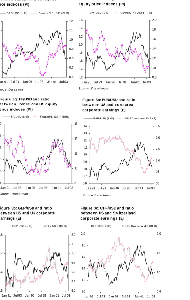
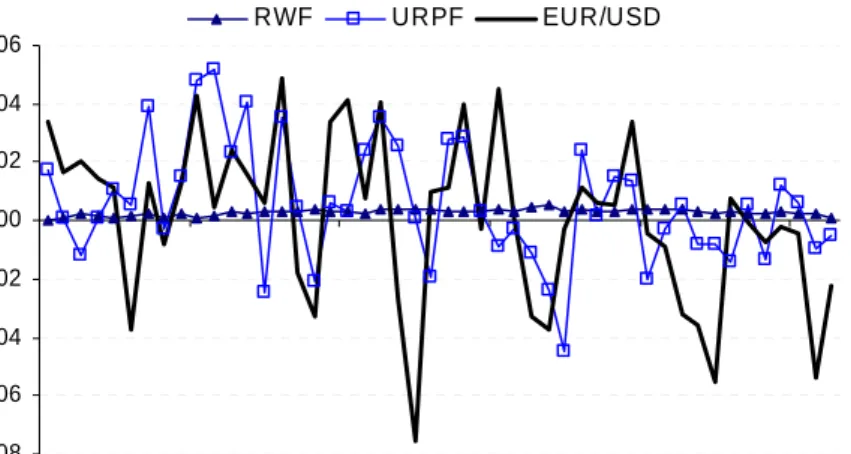
Figures 2a-2g show developments in levels in equity price indices and in the exchange rates of EUR, GBP, CHF, JPY, CAD, DM and FF vis-à-vis the US dollar. Visual inspection suggests that when the euro area equity market exhibits a relatively better performance than the US equity market, the euro tends to depreciate vis-à-vis the US dollar. Similar trends apply to the DM and FF currency pairs against the US dollar. Analogous relationships may be identified when comparing the UK-US equity price ratio and the GBP/USD exchange rate, on the one hand, and the Swiss-US equity price ratio and the CHF/USD exchange rate, on the other hand. Conversely, this relationship becomes quite loose when comparing Japan and Canada with the United States.
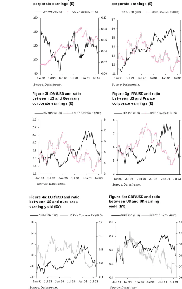
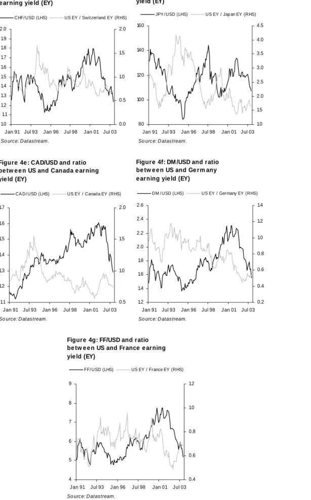
The visual inspection of the relationship between relative cross-country corporate earnings and exchange rates is less informative (see Figures 3a-3g). However, analogous regularities emerge when plotting ratios between country/region earning yields and exchange rates. It seems that, at least over some periods, the exchange rates of the European currencies vis-à-vis the US dollar move in unison with the respective earning yield ratios (see Figures 4a-4g).
5.
Empirical results
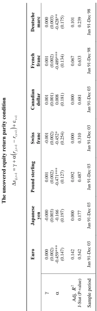
We first test the URP for EUR, GBP, CHF, JPY, CAD, DM and FF, all against the US dollar, assuming that investors are risk neutral. We employ the GMM estimator with a Heteroskedasticity and Autocorrelation Consistent (HAC) covariance matrix.10 Results of equations (3) and (4) are reported in Table 5. In line with the URP, the α coefficients, except for the JPY and CAD, are significantly different from zero and negative, while the γ parameters are not significant. The
9
We also employ other information variables, such as returns lagged up to four periods and a dummy variable which takes on value one each January. For each return differential we select instruments adopting a general-to-specific approach where standard errors are heteroskedasticity and autocorrelation consistent (Newey and West, 1987).
10
We use the standard Bartlett kernel to weigh the autocovariances when computing the weighting matrix. As for the bandwidth selection, we use the fixed Newey-West method for all currency pairs, except for the Swiss franc for which we use the Andrew parameter approach (Andrew, 1991). This methodology assumes that the sample moments follow an AR(1) process.
slopes for the European currencies are less than one in absolute value, suggesting the existence of risk premia, and of about the same magnitude.11 Since the number of moment conditions implied by equation (3) is larger than the number of parameters to estimate, we report a test for the over-identifying restrictions (Hansen, 1982). The p-value of the J-statistic suggests that the null hypothesis that the sample moments in the orthogonality conditions are as close to zero as would be expected if the corresponding population moments were truly zero cannot be rejected at 1% confidence level.
Next we relax the risk neutrality assumption and we proxy the resulting risk premia with economic variables linked to the business cycle: the differential of corporate earnings’ growth rates, net equity flows, the annual inflation rate differentials, and the changes in the short-term interest rate differentials. The econometric specification represented by equations (3) and (5) is tested and results are shown in Table 6.12 Consistently with our previous results, still there exists a significant negative relationship between exchange rate dynamics and equity return differentials, except for the JPY/USD and CAD/USD currency pairs. The estimated risk premia differentials for corporate earnings’ growth rates and net equity flows are positive. As for inflation and interest rate risk premia differentials, the sign is not the same for all currency pairs.
Differentials of growth rates of earnings are one of the driving forces of developments in the European exchange rates. If one country/region grows faster than another, it becomes more attractive to global investors since its assets deliver relatively higher earnings, which, in turn, could result in an appreciation of its currency. We find that currency pair evolution is positively related to corporate earnings growth differentials
(
α2 >0)
in five out of seven cases. The coefficient associated with the change in the corporate earnings growth differential is negative, suggesting a concave relationship vis-à-vis the above mentioned currency pairs.The coefficient associated with net equity flows is positive, but statistically significant only for the EUR/USD and CHF/USD currency pairs.13 The change in inflation differential plays a role only for the EUR/USD exchange rate and the coefficient shows the expected negative sign. The differential in the change of short-term interest rates is important for the evolution of the GBP/USD
11
The URP hypothesis is also tested over the 1980’s. The coefficients of all currency pairs are not significantly different from zero and the regressions do not posses explanatory power. These results are not surprising given the restrictions and the large transaction costs on international capital flows during this period.
12
The British pound depreciated dramatically against the US dollar in September and October 1992, as a result of the European Exchange Rate Mechanism (ERM) crisis (see, for example, Soderlind, 2000). A dummy variable, which is equal to one in September and October 1992, is introduced to capture this intercept shift (see figure 1b).
13
Brooks et al. (2001) obtain similar results analyzing the EUR/USD exchange rate.
and FF/USD exchange rates. The estimated semi-elasticity is positive, which is in line with the prediction of the Dornbush’s (1976) model.
As for the Japanese yen, the URP fairs poorly, possibly due to foreign exchange interventions during the 1990s by Japanese authorities (see, for instance, Ito, 2002, and Nagayasu, 2004). The same argument might apply to the Canadian dollar. Before September 1998, the Canadian Central Bank intervened in the foreign exchange market and the Canadian dollar fluctuated against the US dollar within a moving band (Chen and Rogoff, 2003). Therefore, we exclude the Japanese yen and the Canadian dollar from further analyses.
Since some risk premia are statistically not significant at 10% confidence level, we remove them from the exchange rate specifications using a general-to-specific approach. The resulting parsimonious models are reported in Table 7 and estimates are consistent with those shown in Table 6. We also test whether the coefficients on equity return differentials
( )
α1 and earning growth ratedifferentials
( )
α2 are statistically the same, but of opposite sign. If this is the case and the number of shares is relatively stable, the resulting variable would be equal to the differential in the growth rates of earning yields, ∆(
eyj,t+1−eyi,t+1)
. The null hypothesis α1+α2 =0 cannot be rejected at 5% significance level for the EUR/USD and FF/USD currency pairs and at 1% for the GBP/USD. The test suggests that investors take into consideration earnings yield differentials in deciding their global investment strategies, thereby affecting the dynamics of the exchange rates. In line with the Lucas’s model, a positive domestic real shock (i.e. an increase in domestic earning yields) may determine an appreciation in the domestic currency (see equation (A10)). When earning yields are used as explanatory variables, the point elasticities are positive and statistically significant at 1% confidence level for EUR/USD and FF/USD currency pairs and at 5% for the GBP/USD (see Table 8).The specifications summarized in Table 7 have good explanatory power, as the adjusted coefficients of determination are equal to 24.3% for the EUR/USD, 34.6% for the GBP/USD, and 5.5% for the CHF/USD exchange rates. This is a satisfactory outcome in the view of most previous empirical models, which usually are able to explain little variations in exchange rates. The predictive accuracy of these specifications will be next compared with the predictive accuracy obtained adopting a naïve random walk model.
6.
Can we beat the random walk?
Following a tradition initiated with the seminal paper of Meese and Rogoff (1983), the forecasting ability of the URP specifications reported in Table 7 is compared with the forecasting performance
of a random walk model with drift, where increments are conditionally normally distributed with zero mean and variance σ2t+1:
(6) sij,t+1 =µ+sij,t +εt+1, εt+1ℑt~N
(
0,σt2+1)
.The time-varying variance σ2t+1 is assumed to follow the Generalized Autoregressive
Conditionally Heteroskedastic (GARCH) process proposed by Engle (1982) and Bollerslev (1986):
2 2 2 1 2 1 t t t =ω+λ ε +λ σ σ+ .
Notice that equation (6) represents the most general version of the random walk model, since innovations are supposed to be not identically and not independently distributed, although increments are uncorrelated, i.e. Cov
(
εt,εt−k)
=0, for all k ≠0.14 This representation has been motivated by the fact that financial time series, including exchange rate changes, are usually characterized by volatility clustering.The specifications described in Table (7) have been initially estimated up to December 1998. Next forecasts are carried out at horizons of one, two, three, four, six, nine and twelve months. The model is then estimated again adding one month of data and another set of forecasts is carried out. The procedure is reiterated until December 2002. In line with Meese and Rogoff (1983), the forecasts of the explanatory and instrumental variables – necessary to generate the forecasts of the exchange rates – are not computed; instead, actual realized values are utilized.15 This methodology generates 49 forecast observations of the exchange rates, which can be used to compare predictive accuracy of our suggested model against the random walk.
The Mean Square Error (MSE) is employed to test whether the forecasts obtained with the specifications summarised in Table (7) are more accurate than the forecasts generated with the random walk model (6). The null hypothesis that the two specifications have equal accuracy against the alternative hypothesis that the forecasts generated with one model are more accurate than the forecasts generated with another model is tested with the Modified Diebold-Mariano (MDM)
14
Two other versions of the random walk hypothesis are commonly used in the literature (see Campbell et al., 1997). In the first one it is assumed that innovations are independently and identically distributed, while in the second one increments are independent but not identically distributed. The model described by equation (6) encompasses these two versions as special cases. Notice that since GARCH processes capture the serial correlation of volatility, they permit to relax the independence assumption typical of the first two versions of the random walk hypothesis.
15
As pointed out by Meese and Rogoff (1983), the use of realised values for the explanatory and instrumental variables prevents that the poor predictive power of exchange rate models can be attributed to the difficulties in predicting explanatory and instrumental variables themselves.
statistic of Harvey et al. (1997). The test is based on loss function (MSEs) differentials. The statistic, which has a Student’s t distribution, reads as follows:
(7)
(
)
( )
d Vˆ d n h h n h n MDM 2 1 2 1 2 1 ⎥⎦ ⎤ ⎢⎣ ⎡ + − + − = ,( )
= −(
γ +∑
M= γ)
k mkˆk ˆ n d Vˆ 0 1 1 2 , = −∑
n= t dt n d 1 1 ,where n is the number of forecasts, h the step ahead forecasts, dt the difference between the loss functions under the two alternative models, ˆγ0, ˆγ1, ….., ˆγh−1 the estimated autocovariances, mk the associated weights computed using the Barlett (triangular) window;16 and M the truncation point. M is chosen such that Vˆ
( )
d >0(Diebold and Mariano, 1995). In our case, M is set equal to three.Column (1) of Table 9 reports the ratios between the Root Mean Square Error (RMSE) obtained using the models described in Table 7 and the RMSE computed with the random walk. Our suggested specifications beat the random walk if the statistics are smaller than unity. Column (2) shows the MDM statistics.17 The models we propose beat the random walk if the statistics turn out to be significantly negative. The URP specification forecasts the EUR/USD exchange rate more precisely than the random walk at two- and three-step ahead. The forecasting performances for the Swiss Franc are even better, but they are unsatisfactory for the British Pound.
Leitch and Tanner (1991) underline that the direction of change criterion not only constitutes an alternative forecasting metric, but it is also relevant for profitability and economic concerns. The sign test can be more appropriate than others based on merely statistic motivations. A direction-of-change statistic takes on the value zero if the forecast series correctly predicts the direction of change, and the value one otherwise. The associated loss function reads as follows:
(8)
(
)
( )
( )
( )
( )
⎪⎩ ⎪ ⎨ ⎧ ∆ ≠ ∆ ∆ = ∆ = t , ij t , ij t , ij t , ij t , ij t , ij sˆ sign s sign if sˆ sign s sign if sˆ , s L 1 0 ,where sij,t denotes the actual exchange rate series and sˆij,t its forecast. The likelihood of correctly predicting the directional change, D, can be computed by summing up the number of observations
16
We have also used the Tukey window (where mk =0.5
(
1+cos{
πk M}
)
) as an alternative to the Barlett window(where mk =1−k M ). The results are similar. 17
The autoregressive term in the GBP/USD specification is excluded in order to use the MDM statistic as it is designed for non-nested forecasts. To control for the possibility that sample moments follow an AR(1) process, we employ the parametric method suggested by Andrews (1991) for the bandwidth selection. Nevertheless, the two methods, Andrews and Fixed-Newey-West, yield similar results.
whose value is zero and dividing them by the total number of predictions. When D is significantly larger than 0.5, the forecast has the ability to predict the direction of change. On the other hand, if the statistic is significantly smaller than 0.5, the forecast will tend to give the wrong direction of change. In large samples, it can be shown that the sign test is normally distributed (see Diebold and Mariano, 1995):
(
)
n . . D 25 0 5 0 − ~N( )
0,1 .Directions of changes are accurately predicted for the euro two thirds of the times, but less precisely for the other two currencies (see column (3)). Columns (4) reports the correlation coefficients between the actual and URP-based forecast exchange rate changes, while column (5) shows correlation coefficients associated with the forecasts carried out with the random walk model. Correlations are negative and low when predictions are performed with the random walk specification, while they are positive and particularly large for the EUR/USD exchange rate when the currency dynamics is forecast using the URP models.
Figures 5a-5c compare the evolution of the actual exchange rate for the three European currencies and the two-step ahead forecasts, where predictions are performed with the URP models and the random walk specification. The point forecasts computed with the random walk are represented by a strait line.18 Visual inspection confirms the results presented in columns (4) and (5) of Table 9.
7.
Summary of results and conclusions
Over the last two decades a large number of studies have tried to explain and test the dynamics of exchange rates. Traditional theoretical models of exchange rate determination fare quite poorly when confronted with data and usually show limited forecasting ability, since almost never perform better than a naïve random walk specification. Major innovative contributions are due to microfounded models à la Obstfeld and Rogoff (1995) and the micro-structure literature. Nevertheless, new open-economy macroeconomics frameworks do not seem to be buttressed by solid empirical evidence. As for the micro-structure literature, although the explanatory power of this typology of models increases in comparison to other approaches, the fundamentals driving order flows are not clear.
18
The function representing the forecasts obtained with a random walk model is not a perfectly straight line since the intercept is re-estimated at the beginning of any forecast period.
The increasing role played by international financial markets in developed economies constitutes a persuasive argument to explore possible relationships between returns on risky assets and exchange rates dynamics. Recently, a new strand of research has investigated the interconnections between equity and bond returns, on one side, and exchange rate dynamics, on the other side, with promising results (see Brandt et al., 2001; Pavlova and Rigobon, 2003; Hau and Rey, 2004 and 2005). In this spirit, this paper develops and tests an arbitrage condition, the URP, which finds its theoretical underpinning in the consumption economy of Lucas (1982). The key idea underlying this equilibrium hypothesis is that, in order to arbitrage away profit opportunities, expected changes in exchange rates are linked to differentials in expected returns on equities. We first test the URP assuming risk neutrality and next we relax this hypothesis. Estimating the URP under risk neutrality, we find that a relative increase in equity returns in the euro area, the United Kingdom, Switzerland, Germany and France vis-à-vis the United States is associated with an appreciation of the US dollar against the currencies of these economies.
When we assume that investors are risk-adverse, we use additional explanatory variables proxying for the resulting risk premia, which, in turn, are related to the business cycle. We employ differentials in corporate earnings’ growth rates, short-term interest rate changes, and annual inflation rates, as well as net equity flows. This version of the URP is validated by the data and exhibits good explanatory power.
We also test the forecasting ability of the URP with time-varying risk premia and find that it beats the naïve random walk model with drift at two- and three-month ahead forecasts and always predicts about two thirds of directional changes for the EUR/USD exchange rate. The forecasting performances for the Swiss Franc are better in terms of MSE, but not in terms of the sign test. The specification for the British pound does not beat the naïve random walk model, despite it predicts correctly more than 60% of its directional changes.
Similar specifications fail in explaining the evolution of the Japanese Yen and the Canadian dollar against the US dollar, possibly due to the systematic intervention policy of these countries in the foreign exchange market.
References
Adler, M., and B. Dumas, 1983, “International Portfolio Choice and Corporation Finance: a Synthesis,” Journal of Finance, 38, pp. 925–984.
Andrews, D.W.K. (1991), “Heteroskedasticity and Autocorrelation Consistent Covariance Matrix Estimation,” Econometrica, 59, 817-858.
Arrow, K.J., 1964, “The Role of Securities in the Optimal Allocation of Risk-Bearing,” Review of Economic Studies, 31, pp. 91-96.
Barr, D.G., and R. Priestley, 2004, “Expected Returns, Risk and the Integration of International Bond Markets,” Journal of International Money and Finance, 23, pp. 71-97.
Bollerslev, T., 1986, “Generalized Autoregressive Conditional Heteroskedasticity,” Journal of Econometrics, 31, pp. 307-327.
Brandt, M.W., J.H. Cochrane, and P. Santa-Clara, 2001, “International Risk Sharing is Better than you Think (or Exchange Rates are much too Smooth),” NBER working paper, n. 8404.
Brooks, R., H. Edison, M. Kumar, and T. Slok, 2001, “Exchange Rates and Capital Flows,” IMF working paper, n. WP/01/190.
Campbell, J.Y., A.W. Lo, and A.C. MacKinlay, 1997, The Econometrics of Financial Markets, Princeton University Press, Princeton, NJ.
Chen, N.F. (1991), “Financial Investment Opportunities and the Macroeconomy”, Journal of Finance, 46, pp. 529-554.
Chen, Y. and K. Rogoff, 2003, “Commodity Currencies,” Journal of International Economics, 60, pp. 133-160.
Debreu, G., 1959, Theory of Value, Yale University Press, New Haven, CT.
Diebold, F.X., and R. Mariano,1995, “Comparing Predictive Accuracy,” Journal of Business and Economic Statistics, 13, pp. 253-265.
Dornbusch, R., 1976, “Expectations and Exchange Rate Dynamics,” Journal of Political Economy, 84, pp. 1161-1176.
Engel, C., 1996, “The Forward Discount Anomaly and the Risk Premium: A Survey of recent Evidence,” Journal of Empirical Finance, 3, pp. 123-192.
Engle, R., 1982, “Autoregressive Conditional Heteroskedasticity with Estimates of the Variance of UK Inflation,” Econometrica, 50, pp. 987-1008.
Evans, M.D.D., and R.K. Lyons, 2002, “Order Flow and Exchange Rate Dynamics,” Journal of Political Economy, 110, pp. 170-180.
Fama, E.F., 1984, “Forward and Spot Exchange Rates,” Journal of Monetary Economics, 14, pp. 319-338.
Fama, E.F., and K. French, 1989, “Business Conditions and Expected Returns on Stocks and Bonds,” Journal of Financial Economics, 25, pp. 23-49.
Ferson, W.E. and C.R. Harvey, 1991a, “Sources of Predictability in Portfolio Returns,” Financial Analysts Journal, May-June, pp. 49-56.
Ferson, W.E. and C.R. Harvey, 1991b, “The Variation of Economic Risk Premiums,” Journal of Political Economy, 99, pp. 385-415.
Frankel, J.A., and A.K. Rose, 1995, “Empirical Research on Nominal Exchange Rates,” in G. Grossman and K. Rogoff (eds.), Handbook of International Economics, vol. III, Amsterdam: Elsevier Science, pp. 1689-1729.
Hansen, L.P., 1982, “Large Sample Properties of Generalized Method of Moments Estimators,” Econometrica, 50, pp. 1029-1054.
Harvey, D., S. Leybourne, and P. Newbold, 1997, “Testing the Equality of Prediction Mean Squared Errors,” International Journal of Forecasting, 13, pp. 281-291.
Hau, H., and H. Rey, 2004, “Can Portfolio Rebalancing Explain the Dynamics of Equity Returns, Equity Flows, and Exchange Rates?” American Economic Review Paper and Proceedings, 94, pp. 126-133.
Hau, H., and H. Rey, 2005, “Exchange Rate, Equity Prices and Capital Flows,” forthcoming Review of Financial Studies.
Hodrick, R.J., 1987, The Empirical Evidence of the Efficiency of Forward and Futures Foreign Exchange Markets, Harwood academic publishers, Chur.
Ito, T., 2002, “Is Foreign Exchange Intervention Effective?: The Japanese Experiences in the 1990s”, NBER Working Paper, n. 8914.
Kirby, C., 1997, “Measuring the Predictable Variation in Stock and Bond Returns,” Review of Financial Studies, 10, pp. 579-630.
Leitch, G., and J.E. Tanner, 1991, “Economic Forecast Evaluation: Profits versus the Conventional Error Measures,” American Economic Review, 81, pp. 580–590.
Lucas, R.E. Jr., 1982, “Interest Rates and Currency Prices in a Two-Country World”, Journal of Monetary Economics, 10, pp. 335-359.
Lyons, R.K., 1995, “Tests of Microstructural Hypotheses in the Foreign Exchange Markets,” Journal of Financial Economics, 39, pp. 321-351.
Lyons, R.K., 2001, The Microstructure Approach to Exchange rates, The MIT Press, Cambridge. Meese, R., and K. Rogoff, 1983, “Empirical Exchange Rates Models of the Seventies: Do they fit
out of sample,” Journal of International Economics, 14, pp. 3-24.
Nagayasu, J., 2004, “The Effectiveness of Japanese Foreign Exchange Interventions During 1991-2001”, Economics Letters, 84, pp. 377-381.
Newey, W.K. and West, K.D., 1987, “A Simple, Positive Definite, Heteroskedasticity and Autocorrelation Consistent Covariance Matrix”, Econometrica, 55, pp. 703-708.
Obstfeld, R., and K. Rogoff, 1995, “Exchange Rates Dynamics Redux,” Journal of Political Economy, 103, pp. 624-660.
Pavlova, A., and R. Rigobon, 2003, “Asset Prices and Exchange Rates,” NBER working paper, n. 9834.
Soderlind, P., 2000, “Market Expectations in the UK Before and After the ERM Crisis”, Economica, 67, pp. 1-18.
Solnik, B., 1974, “An Equilibrium Model of the International Capital Market,” Journal of Economic Theory, 8, pp. 500–524.
Taylor, M.P., 1995, “The Economics of Exchange Rates,” Journal of Economic Literature, 33, pp. 13-47.
Appendix A: The URP condition in Lucas’ consumption economy
In this appendix we sketch Lucas’ (1982) consumption economy model and next we derive the URP condition.
Assume that the world consists of two countries, i and j, and that in each country there are infinitely-lived consumers. Agents in the two countries exhibit identical preferences, which are defined over the infinite stream of two consumption goods, x and y, and are risk averse.19 Consumers, however, have different stochastic endowments of the two goods. At time t, each citizen of country i is endowed with ξt units of a freely transportable, non storable consumption good x and nothing of commodity y, while each citizen of country j is endowed with ηt units of the second good y and nothing of commodity x. The realizations ξt and ηt completely describe the current real state of the system. Moreover, the stochastic bivariate process
(
ξt,ηt)
is assumed to be drawn from a unique stationary Markov distribution F(
ξt,ηtξt−1,ηt−1)
which gives the transition probability of ξt and ηt conditional on ξt−1 and ηt−1.The representative agent’s preferences are expressed by the following expected utility function: (A1)
(
)
⎭ ⎬ ⎫ ⎩ ⎨ ⎧ β ℑ = ∞ =∑
0 0 t t lt lt t y , x U E ,where E
{ }
⋅⋅ is the expectation operator conditional on the information set ℑt=0, β is the commondiscount factor, 0<β<1, while xltand ylt represent consumption of the good x and y, respectively, in country l = i, j at time t. The utility function is assumed to be bounded, continuously differentiable, increasing in both arguments, and strictly concave. Markets are supposed to be complete in the sense of Arrow (1964) and Debreu (1959), which means that agents trade in both goods contingent of all possible realization of the stochastic process
(
ξt,ηt)
.The use of money or currency is introduced by assuming that agents can purchase the endowment of a country only with the currency of that country. Let Mt be the period t per capita quantity of money of country i, say the nominal euro, and let Nt be the period t per capita quantity of the money of country j, say the nominal US dollars. Define wit,
( )
wjt, as the exogenous stochastic rate of change in money. Prior to any trading at time t, suppose that each trader in country
19
The fact that agents are risk averse will enrich the URP with risk premia.
i receives a lump sum euro transfer of wi,tMt−1 and, similarly, each trader in country j a lump sum dollar transfer of wj,tNt−1 so that the money supply evolves as follows:
(A2) Mt+1 =
(
1+wi,t+1)
Mt, (A3) Nt+1 =(
1+wj,t+1)
Nt.20The equilibrium nominal prices of goods x and y in terms of domestic and foreign currency, as well as ξt and ηt are given by:
(A4)
( )
t t t t , x M M P ξ = , (A5)( )
t t t t , y N N P η = .Maximizing the expected present value of the representative agent’s utility function, subject to budget constraints and cash-in-advance constraints gives a set of first order conditions (see Lucas, 1982, for further details). These include the standard requirement that the marginal rate of substitution between domestic and foreign goods equals their relative prices, and the Euler equations for xth and yth stocks:
(A6)
(
)
(
t t)
t , x t t t , y t , y y , x U y , x U p = , (A7)( )
( )
dFdK w q U q U t , i t t , x t , x t , x t , x∫
⎥ ⎦ ⎤ ⎢ ⎣ ⎡ + ξ + ⋅ β = ⋅ + + + + 1 1 1 1 1 , (A8)( )
( )
p dFdK w q U q U y,t t , j t t , x t , x t , y t , x∫
⎥ ⎥ ⎦ ⎤ ⎢ ⎢ ⎣ ⎡ + η + ⋅ β = ⋅ + + + + + 1 1 1 1 1 1 . t, yp is the relative domestic spot price of y in terms of the numeraire x,
(
t t)
(
t t)
tt ,
y x ,y U x ,y y
U ≡∂ ∂ , Ux,t
(
xt,yt)
≡∂U(
xt,yt)
∂xt, qxt, is the current price, in x-unit, of a claim to the entire future stream{ }
ξt t∞=t+1 of the endowment of good x, and qyt, is the current domestic price, in x-unit, of a claim to the entire future stream{ }
ηt ∞t=t+1 of the endowment of good y.
20
The transition function for the process
{ }
wt ={
wi,t,wj,t}
is also a known Markov process K[
wtwt−1,F(
ξt,ηtξt−1,ηt−1)
]
which gives the transition probability of wt conditional on wt−1 and the probability of the future real state given by( )
⋅⋅ F .Notice that qxt, and qyt, are expressed in domestic currency. Therefore, pyt,, qxt, and qyt, are real prices expressed in domestic currency.
The nominal exchange rate enters the model because the Purchasing Power Parity (PPP) holds: (A9)
(
) ( )
( )
t t , x t t , y t t t , ij t , y M P N P N , M S p = ,where Sij,t
(
Mt,Nt)
is the nominal spot exchange rate of currency i with respect to currency j, that is the number of units of currency i exchanged for one unit of currency j (for instance euro per US dollars).Rearranging (A9) and using (A6) give the nominal exchange rate:
(A10)
(
)
(
(
)
)
t t t t t t t, x t t t, y t t t, ij N M y , x U y , x U N , M S ξ η = .The fundamental determinants of the nominal exchange rate are relative money supplies and relative endowments. In addition, the exchange rate depends also on consumer preferences.
Lucas’ model can be extended and the URP derived. We use the Euler equations to build a relationship between expectations in exchange rate dynamics and expected equity returns in the two countries.
Combining (A7) and (A8) yields:
(A11)
( )
( )
p dFdK w q U q dFdK w q U q j,t y,t t t , y t , x t , y t , i t t , x t , x t , x∫
∫
⎥ ⎥ ⎦ ⎤ ⎢ ⎢ ⎣ ⎡ + η + ⋅ = ⎥ ⎦ ⎤ ⎢ ⎣ ⎡ + ξ + ⋅ + + + + + + + + + 1 1 1 1 1 1 1 1 1 1 1 1 1 .Using (A2) and (A4) on the left-hand side of (A11), and (A3), (A5) and (A9) on the right-hand side of (A11), the above equality becomes:
(A12)
( )
( )
( )
(
)
( )
( )
( )
(
)
dFdK, M P M P S S Q N P Q Q U dFdK M P M P Q M P Q Q U t t, x t t, x t, ij t, ij t, y t t, y t t, y t, y t, x t t, x t t, x t, x t t, x t t, x t, x t, x∫
∫
+ + + + + + + + + ⎥ ⎥ ⎦ ⎤ ⎢ ⎢ ⎣ ⎡ η + ⋅ = ⎥ ⎦ ⎤ ⎢ ⎣ ⎡ ξ + ⋅ 1 1 1 1 1 1 1 1 1where Qxt, is the current nominal price of a claim to the entire future stream
{ }
∞+ =
ξt t t 1 of the endowment of good x expressed in domestic currency, and Qyt, the current nominal foreign price of a claim to the entire future stream
{ }
ηt t∞=t+1 of the endowment of good y expressed in foreign currency.Since gross total returns may be defined as 1+Rxt,+1=
[
Qxt,+1+ξtPxt,( )
Mt]
Qxt, and( )
[
yt, t yt, t]
yt, t, y Q P N Q R = +η + +1 +11 , being ξtPx,t
( )
Mt and ηtPyt,( )
Nt the nominal dividends at time t in the domestic and foreign economy, respectively, while the gross inflation rate is equal to= π + +1
1 t Px,t+1
(
Mt+1)
Px,t( )
Mt , equation (A12) can be expressed as:(A13)
( )(
)
(
)
( )(
)
(
)
dFdK S S R U dFdK R U t, ij t, ij t, y t t, x t, x t t, x∫
∫
+ + − + + + − + + ⋅ +π + = ⋅ +π + 1 1 1 1 1 1 1 1 1 1 1 1 1 .Equation (A13) can be re-written making use of the conditional expectation operator:
(A14)
{
( )(