Classical time-varying FAVAR models –
estimation, forecasting and structural analysis
Sandra Eickmeier
(Deutsche Bundesbank)
Wolfgang Lemke
(European Central Bank and Deutsche Bundesbank)
Massimiliano Marcellino
(European University Institute, Florence, Università Bocconi, Milano and CEPR)
Discussion Paper
Series 1: Economic Studies
No 04/2011
Editorial Board: Klaus Düllmann
Frank Heid
Heinz Herrmann
Karl-Heinz Tödter
Deutsche Bundesbank, Wilhelm-Epstein-Straße 14, 60431 Frankfurt am Main, Postfach 10 06 02, 60006 Frankfurt am Main
Tel +49 69 9566-0
Telex within Germany 41227, telex from abroad 414431
Please address all orders in writing to: Deutsche Bundesbank,
Press and Public Relations Division, at the above address or via fax +49 69 9566-3077
Internet http://www.bundesbank.de
Reproduction permitted only if source is stated.
ISBN 978-3–86558–692–6 (Printversion) ISBN 978-3–86558–693–3 (Internetversion)
Abstract
We propose a classical approach to estimate factor-augmented vector autoregressive (FAVAR) models with time variation in the factor loadings, in the factor dynamics, and in the variance-covariance matrix of innovations. When the time-varying FAVAR is estimated using a large quarterly dataset of US variables from 1972 to 2007, the results indicate some changes in the factor dynamics, and more marked variation in the factors' shock volatility and their loading parameters. Forecasts from the time-varying FAVAR are more accurate than those from a constant parameter FAVAR for most variables and horizons when computed in-sample, for some variables in pseudo real time, mostly financial indicators. Finally, we use the time-varying FAVAR to assess how monetary transmission to the economy has changed. We find substantial time variation in the volatility of monetary policy shocks, and we observe that the reaction of GDP, the GDP deflator, inflation expectations and long-term interest rates to an equally-sized monetary policy shock has decreased since the early-1980s.
JEL: C3, C53, E52
Non-technical summary
The recent macroeconometric literature has seen an increasing interest in the application of factor-augmented vector autoregressive (FAVAR) models for forecasting and structural analysis. These models provide a means to exploit large information sets and handle the omitted-variable problem often encountered in standard small-scale vector autoregressive (VAR) models. FAVARs model a large number of variables as the sum of a common component and an idiosyncratic component. The common component of a variable is the product of a few common factors, representing the main driving forces underlying most economic variables, and variable-specific factor loadings. The factors are assumed to follow a VAR process. The parameters are typically assumed to be constant over time in this literature.
Another recent strand of literature has focused on small models with time-varying parameters, to explicitly take into consideration the changing sources of economic fluctuations, i.e. changes in the sizes of shocks and in their transmission to the economy. This literature therefore meets concerns about structural changes in the economy stemming from sources such as financial deepening, globalization or institutional changes.
A few papers have attempted to combine the FAVAR and the time-varying parameter approaches, introducing FAVAR models with time-varying parameters, hence combining the benefits of using lots of variables and allowing for a time-varying model structure. All existing contributions use Bayesian procedures for estimation. Instead, in this paper we propose a fully classical approach to estimating a FAVAR model with time-varying parameters. Our time-varying version is fairly flexible, as it can accommodate smooth changes in the factor loadings, in the autoregressive coefficients of the factor VAR, in the contemporaneous relationships between the factors, and in the volatility of the common shocks.
We estimate the time-varying FAVAR (TV-FAVAR) in two stages. The first stage involves estimating the factors with principal components (PC). The PC estimator is consistent for the factors even if the loadings mildly vary over time. The second stage involves estimating the time-varying loading coefficients, the autoregressive matrices of the factor VAR as well as the time-varying variances and correlations. A representation for the VAR with a lower-triangular matrix of contemporaneous relations is employed, which renders the VAR
equations conditionally independent, and the common shock volatilities are modelled as functions of lagged factors. The model is then estimated equation-wise by Maximum Likelihood based on the Kalman filter.
As an empirical example, we fit our TV-FAVAR to a large quarterly US dataset with more than 300 macroeconomic and financial variables, observed between 1972 and 2007. Our estimation results imply substantial time variation in the variance of the shocks but also in the system dynamics, as represented by the factor loadings and factor dynamics.
We then use the model to produce in- and out-of-sample forecasts of various macroeconomic and financial variables. In general, it turns out that for most variables and forecast horizons the forecasts from the TV-FAVAR are more accurate than those from a constant-parameter FAVAR. The results deteriorate somewhat in a post-1995 pseudo real time analysis, but the TV-FAVAR still dominates for most monetary and financial variables.
Finally, we contribute to the growing literature on time variation in the monetary transmission mechanism by identifying monetary policy shocks and assessing their transmission to the US economy over time. We confirm the finding of previous studies that the volatility of the monetary shocks is substantially smaller after the early-1980s. The negative impact of a same-sized contractionary shock on most activity and price measures has declined over time. The effects on activity variables do not appear to be different during recessionary phases compared to expansions. Finally, the negative impact of monetary policy shocks on inflation expectations and long-term interest rates has weakened over time. This could be due to changes in the conduct of monetary policy which reacts since the beginning of the 1980s more strongly to output and price fluctuations which, in turn, has led to better anchored inflation expectations. Another possible explanation is globalization in the course of which the effect of domestic shocks on long-term interest rates has decreased at the expense of foreign shocks. Both the declined impact on inflation expectations and long-term rates may have contributed to the decline in the impact on activity and prices.
Nichttechnische Zusammenfassung
Die jüngere makroökonometrische Literatur interessiert sich zunehmend für Anwendungen so genannter ‚factor-augmented vector autoregressive (FAVAR) models’ für die Prognose und strukturelle Analysen. Diese Modelle sind in der Lage, umfangreiche Datenmengen zu nutzen und insofern Probleme aufgrund ausgelassener Variablen zu vermeiden, welche häufig in kleineren Vektor-autoregressiven Modellen (VARs) auftreten. In FAVAR-Modellen wird die gemeinsame Entwicklung einer Vielzahl von Variablen erfasst. Dabei wird jede Variable als Summe einer gemeinsamen und einer variablenspezifischen Komponente modelliert. Die gemeinsame Komponente ist das Produkt weniger gemeinsamer Faktoren, die die wesentlichen ökonomischen Einflussgrößen erfassen, und sog. Faktorladungen, die variablenspezifisch sind. Die zeitliche Entwicklung der Faktoren wird mit Hilfe eines VARs abgebildet. Es wird in der Literatur üblicherweise angenommen, dass die Modellparameter über die Zeit konstant sind.
Ein anderer Literaturstrang nutzt kleine Modelle mit zeitvariierenden Parametern, um explizit sich verändernde Ursachen und Mechanismen wirtschaftlicher Schwankungen zu untersuchen. Diese Änderungen beziehen sich auf die Größe der ‚Schocks’ (unerwartete Änderungen der betrachteten Variablen) sowie deren direkte und mittelbare Auswirkungen auf die Volkswirtschaft. Diese Literatur trägt somit der Existenz struktureller Veränderungen Rechnung, wie beispielsweise einer stärkeren Bedeutung des Finanzsektors, der Globalisierung oder institutioneller Änderungen.
Einige wenige Papiere haben FAVAR-Modelle und die zeitvariierenden Parameteransätze kombiniert und FAVAR-Modelle mit zeitvariierenden Parametern (TV-FAVAR) eingeführt. Alle existierenden Beiträge verwenden Bayesianische Schätzmethoden. In diesem Papier schlagen wir stattdessen ein vollständig klassisches Schätzverfahren für FAVAR-Modelle mit zeitvariierenden Parametern vor. Unser zeitvariables Model ist recht flexibel, denn es erlaubt graduelle Veränderungen in den Faktorladungen, in den autoregressiven Koeffizienten des Faktor-VARs, in den kontemporären Beziehungen zwischen den Faktoren sowie der Volatilität der gemeinsamen Schocks.
Wir schlagen vor, das TV-FAVAR in zwei Schritten zu schätzen. In einem ersten Schritt werden die Faktoren mit Hilfe einer Hauptkomponentenanalyse (HK) bestimmt. Der
HK-Schätzer ist konsistent für die Faktoren, selbst wenn die Faktorladungen sich über die Zeit (begrenzt) verändern. In einem zweiten Schritt werden die zeitvariierenden Ladungen, die autoregressiven VAR-Parameter, die Korrelationen und Schockvarianzen geschätzt. Wir wählen eine Repräsentation des VARs, bei der die kontemporären Beziehungen zwischen den Faktoren einer unteren Dreiecksmatrix entsprechen, so dass die einzelnen Gleichungen des VARs (bedingt) unabhängig voneinander sind. Die Volatilitäten der gemeinsamen Schocks werden als Funktionen der verzögerten Faktoren modelliert. Das Modell kann dann Gleichung für Gleichung mit Maximum Likelihood, basierend auf dem Kalman Filter geschätzt werden.
Wir wenden unser TV-FAVAR auf einen großen vierteljährlichen Datensatz mit über 300 US-amerikanischen makroökonomischen und Finanzmarktvariablen zwischen 1972 und 2007 an. Unsere Schätzergebnisse zeigen ausgeprägte Zeitvariation in der Varianz der gemeinsamen Schocks, aber auch im Transmissionsmechanismus, welcher durch die Ladungen und die Faktordynamik abgebildet wird.
Das Modell wird anschließend genutzt, um verschiedene makroökonomische und Finanzmarktvariablen zu prognostizieren. Für die meisten betrachteten Variablen und Vorhersagehorizonte ist die Prognosegüte des TV-FAVAR der von FAVAR Modellen mit konstanten Parametern überlegen. In einer (‚pseudo’-) Echtzeit-Prognose für die Quartale ab 1995 verschlechtert sich die relative Vorhersagequalität des TV-FAVAR etwas, allerdings dominiert das Modell alternative Ansätze bei der Vorhersage der meisten monetären Aggregate und Finanzmarktvariablen.
Schließlich untersuchen wir, wie sich die geldpolitische Transmission auf die US-Wirtschaft mit der Zeit verändert hat. Wie auch vorangegangene Studien finden wir, dass die Volatilität geldpolitischer Schocks ab Mitte der Achtziger Jahre geringer ist als davor. Der negative Effekt eines kontraktiven geldpolitischen Schocks (vergleichbarer Größe) auf die Realwirtschaft und auf Preise ist im Allgemeinen mit der Zeit kleiner geworden. Wir finden keinen Hinweis darauf, dass sich geldpolitischer Schocks stärker auf die Realwirtschaft in Rezessionen als in konjunkturellen Aufschwungphasen übertragen. Schließlich scheinen sich der negative Effekt kontraktiver geldpolitischer Schocks auf Inflationserwartungen und der positive Effekt auf Langfristzinsen über die Zeit abgeschwächt zu haben. Dies liegt möglicherweise in Veränderungen in der Politik der Zentralbank begründet, die seit Beginn der Achtziger Jahre aggressiver auf Schwankungen in der Realwirtschaft und bei den Preisen
reagiert, was wiederum zu stärker verankerten Inflationserwartungen geführt haben mag. Ein weiterer Erklärungsfaktor könnte die Globalisierung sein, in deren Folge der Einfluss heimischer Schocks zu Lasten globaler Schocks abgenommen haben könnte. Der geringere Effekt auf Inflationserwartungen und Langfristzinsen kann möglicherweise auch den rückläufigen Effekt geldpolitischer Schocks auf Aktivität und Preise erklären.
Contents
1 Introduction 1
2 The TV-FAVAR model: representation and estimation 4
2.1 The TV-FAVAR model 4
2.2 Estimating the TV-FAVAR 6
2.3 Comparison with related approaches 9
3 A large dataset for the US 10
4 Estimation results 11
4.1 Estimated factors 11
4.2 Time variation in parameters and volatility 12
4.3 Diagnostic checking 13
5 Forecasting with the TV-FAVAR 13
5.1 In-sample forecasts 14
5.2 Out-of-sample forecasts 16
6 Structural analysis 17
6.1 Possible reasons for changes in the monetary transmission mechanism
and existing empirical evidence 17
6.2 Monetary policy shock identification 18
6.3 Computing time-varying impulse responses 19
6.4 Monetary policy shocks and transmission in our TV-FAVAR 20
7 Conclusions 22
Tables and Figures
Table 1: Tests for autocorrelation of the idiosyncratic errors 27
Table 2: In-sample forecast results 28
Table 3: Out-of-sample forecast results 31
Table 4: Overview of existing studies on changes in the
monetary transmission mechanism in the US 34
Figure 1: Factor estimates 36
Figure 2: Autocorrelation function of the standardized VAR residuals 36
Figure 3: Time-varying volatility of the monetary policy shock 36
Figure 4: Impulse response functions of key variables 37
Figure 5: Impulse response functions of additional activity and price variables 38 Figure 6: Impulse response functions of inflation expectations and long-term
government bond yields 40
1
Introduction *
The recent macroeconometric literature has seen an increasing interest in the applica-tion of factor-augmented vector autoregressive (FAVAR) models for forecasting and
struc-tural analysis.1 They provide a means to exploit a large information set and handle the
omitted-variable problem often encountered in standard vector autoregressive (VAR) mod-els. FAVARs were originally suggested by Bernanke et al. (2005), who modeled a large number of variables as the sum of a common component and an idiosyncratic compo-nent. The common component of a variable is the product of a few common factors and variable-specific factor loadings. The factors, the driving forces underlying most economic variables, are assumed to follow a VAR process.
Another recent strand of literature has focused on small models with time-varying parameters, including evolving variances, to explicitly take into consideration the changing sources and sizes of shocks, and their transmission to the economy, see e.g. Cogley and Sargent (2005) and Sims and Zha (2006).
A few papers have attempted to combine the FAVAR and the time-varying parameter approaches, introducing FAVAR models with time-varying parameters, hence combining the benefits of using lots of variables and allowing for a time-varying model structure. Examples include Baumeister et al. (2010) and Korobilis (2009), whose applications con-cern the transmission mechanism of monetary policy in the US, as well as Del Negro and Otrok (2008), Liu and Mumtaz (2009) and Mumtaz and Surico (forthcoming), who fit time-varying FAVAR models to study international business cycle and inflation comove-ments. A common feature of all these contributions is the use of Bayesian procedures. Instead, in this paper we propose a fully classical approach to estimate a FAVAR model with time-varying parameters. Our time-varying version is fairly flexible, as it can
ac-*0The views expressed in this paper do not necessarily represent the view of the European Central Bank or the Deutsche Bundesbank. Sandra Eickmeier thanks the Monetary Policy Strategy Division of the ECB for its hospitality. We thank Christiane Baumeister for useful discussions and for providing us with commodity and PCE price data. We thank Herman van Dijk, Hashem Pesaran, Lucrezia Reichlin, Jim Stock, Harald Uhlig, Giovanni Urga, Mark Watson, as well as participants at the NBER Summer Institute 2010 (Boston) and the conference on ‘High-dimensional econometric modelling’ at Cass Business School (London) and seminar participants at the Deutsche Bundesbank and the European Central Bank for useful discussions. Many thanks go also to Guido Schultefrankenfeld and Michael Richter for their help on the datasets.
1
For forecasting applications see, e.g., Stock and Watson (2002a), Stock and Watson (2002b), Stock and Watson (2006), Eickmeier and Ziegler (2008). Regarding structural analysis see, e.g., Bernanke, Boivin, and Eliasz (2005), Boivin, Kiley, and Mishkin (forthcoming), Baumeister, Liu, and Mumtaz (2010) (for monetary policy applications) and Kose, Otrok, and Whiteman (2003), Kose, Otrok, and Whiteman (2008), Eickmeier (2007), Mumtaz and Surico (2009), Liu and Mumtaz (2009), Del Negro and Otrok (2008), Beck, Hubrich, and Marcellino (2009) (for applications on international business cycle and inflation comovements).
commodate smooth changes in the factor loadings, in the autoregressive coe!cients of the factor VAR, in the contemporaneous relationships between the factors, and in the volatility of the common shocks.
We suggest to estimate the time-varying FAVAR (TV-FAVAR) in two stages. The first stage involves estimating the factors with principal components (PC). As argued by Stock and Watson (2008) and Banerjee, Marcellino, and Masten (2008), the PC estimator is con-sistent for the factors even if the loadings mildly vary over time. The second stage involves
estimating the time-varying loading coe!cients, the autoregressive matrices of the factor
VAR as well as the time-varying variances and correlations. Treating the estimated factors as given, the relations between the observable variables and the factors are represented as a set of univariate regression models with time-varying parameters, which evolve as inde-pendent random walks. As such, the model is estimated equation-wise by converting each equation into state space form, estimating the hyperparameters by maximum likelihood, and applying the Kalman filter to back out the time-varying parameter paths, see e.g. Nyblom (1989). Regarding the time-varying factor VAR, we employ a representation with a lower-triangular matrix of contemporaneous relations, which renders the VAR equations conditionally independent. This again enables us to estimate the model equation-wise, ap-plying standard methods for univariate regression models with time-varying parameters. Concerning the volatility specification, we deviate from the common assumption in the literature that volatility is driven by an additional latent factor. We rather specify it as an
(exponentially a!ne) function of lagged factors, which makes our VAR equations
condi-tionally linear. The resulting estimated pattern of volatility is similar to that returned by models, in which time-varying volatility is captured by additional latent variables. More-over, we think that linking the evolution of volatility to the underlying economic forces, namely, the factors, is a sensible modeling choice.
As an empirical example, we fit our TV-FAVAR to a large quarterly US dataset with more than 300 macroeconomic and financial variables, observed between 1972 and 2007. Our estimation results imply substantial time variation in the variance of the shocks but also in their transmission mechanism, as represented by the factor loadings and factor dynamics. However, time variation is ‘sparse’ in the sense that changes in only a few parameters govern the time variation of the system, while most parameters turn out to be essentially constant over time.
We then use the model to produce in- and out-of-sample forecasts of various macro-economic and financial variables. In the in-sample analysis, we not only look at average forecast errors over the entire sample period but also forecasts for recession periods only, which are notoriously hard to predict with small constant-parameter approaches, as well as forecasts for the post-1995 period for which many models have been shown to perform particularly badly, see D’Agostino, Giannone, and Surico (2007). In general, it turns out that for most variables and forecast horizons the in-sample forecasts from the TV-FAVAR
are more accurate than those from a constant-parameter FAVAR. The results deteriorate in a post-1995 pseudo real time analysis, since estimation uncertainty increases for the TV-FAVAR, while recursive estimation introduces a form of parameter time variation in the constant-parameter FAVAR. However, the TV-FAVAR still dominates for most monetary and financial variables.
Finally, we contribute to the growing literature on time variation in the monetary transmission mechanism by identifying monetary policy shocks and assessing their
trans-mission to the US economy over time.2 3
Boivin et al. (forthcoming) comprehensively overview the existing literature and show that a consensus on how the monetary transmission mechanism in the US has evolved
is still lacking. The time-varying framework also allows us to examine the evolution
of the volatility of monetary policy shocks. We focus on three questions regarding the monetary transmission. (i) Has the transmission to key macroeconomic variables changed over time and, if yes, how? (ii) Can we detect asymmetries or, more specifically, are monetary policy shocks transmitted to economic activity more strongly during recessions than during booms? (iii) Has the transmission to inflation expectations changed over time and, if yes, how?
The results highlight interesting patterns of time variation. In particular, the volatility of the monetary shocks is substantially smaller after the early-1980s. The negative impact of a same-sized shock on most activity and price measures has declined over time. The
eects on activity variables do not appear to be dierent during recessionary phases
com-pared to expansions. Finally, the negative impact of monetary policy shocks on inflation expectations and long-term interest rates has weakened over time. This could be due to changes in the conduct of monetary policy or to globalization and may have contributed to the decline in the impact on activity and prices.
The paper is organized as follows. In section 2 we present the model and estimation methodology and compare our approach with related TV-FAVARs. In section 3 we present the data. In section 4 we fit the TV-FAVAR to the data and present evidence on time variation in the parameters. In section 5 we evaluate the forecasting performance of the TV-FAVAR model. In section 6 we assess changes in the monetary transmission mechanism in the US over time. Finally, in section 7 we summarize the main results and conclude.
2
Especially with this application in view, our sample ends before the onset of the 2007-09 financial crisis. As the Federal Reserve employed a number of non-standard monetary policy measures in reaction to the crisis, it would probably be intricate to interpret results based on shocks to the Federal Funds Rate as the monetary policy instrument during the crisis period.
3
In a companion paper, Eickmeier, Lemke, and Marcellino (2011), we use the TV-FAVAR to trace the eects of US financial shocks on several advanced economies, with a focus on the 2008-2009 financial crisis.
2
The TV-FAVAR model: representation and estimation
In this section we introduce the TV-FAVAR model, discuss its estimation, and compare it to related approaches.2.1
The TV-FAVAR model
Our starting specification is the FAVAR model as proposed by Bernanke et al. (2005). Let [w0 = ({1>w> = = = > {Q>w) denote a large vector of Q zero-mean stationary variables, for
w = 1> = = = > W, where both Q and W can go to infinity. In the standard dynamic factor
model, each element of[wis assumed to be the sum of a linear combination ofJcommon
factorsIw0 = (i1>w> = = = > iJ>w) and an idiosyncratic componenthl>w. Hence,
{l>w =0lIw+hl>w> l= 1> = = = Q> (2.1)
where h0w= (h1>w> = = = > hQ>w). We assume that the factors are orthonormal and uncorrelated
with the idiosyncratic errors, and H(hw) = 0, H(hwh0w) =U, where U is a diagonal matrix.
These assumptions identify the model and are common in the FAVAR literature. They can be partly relaxed when the goal of the analysis is purely factor estimation by means of non-parametric methods, see e.g. Stock and Watson (2002b) and Stock and Watson (2002a).
The dynamics of the factors are then modeled as a VAR(s),
Iw=E1Iw31+= = = EsIw3s+zw> H(zw) = 0> H(zwz0w) =Z= (2.2)
Since each {l>w is assumed to be a zero-mean process (and the respective data are
de-meaned), equations (2.1) and (2.2) do not contain intercepts.
The VAR equation (2.2) can be interpreted as a reduced-form representation of a system of the form
S Iw=K1Iw31+= = =KsIw3s+xw> H(xw) = 0> H(xwx0w) =V> (2.3)
where S is lower-triangular with ones on the main diagonal, and V is a diagonal matrix.
The relation to the reduced-form parameters in (2.2) isEl=S31Kl andZ =S31VS310.
This system of equations may in other contexts be referred to as a ‘structural VAR’ (SVAR) representation. While we will actually use a triangular contemporaneous relation in our structural analysis in section 6, we emphasize that the chosen representation (2.3)
mainly serves to render its J equations conditionally independent. This representation
is particularly useful for estimating the time-varying version outlined below, but after estimation of the system matrices other forms of shock identification besides the specific triangular one may be applied.
Having introduced the standard FAVAR model with a constant parameter structure, we now relax the assumption of parameter constancy in four dimensions. Specifically, we
allow for time variation in: (i) the autoregressive dynamics of the factors (K1> = = = >Ks),
(ii) the contemporaneous relations captured by the matrixS , (iii) the variances of factor
innovations, i.e., the elements ofV in (2.3), and (iv) the factor loadings in (2.1). Thus, we
consider the following time-varying version of (2.1) and (2.3):
{l>w =0l>wIw+hl>w> l= 1> = = = > Q (2.4)
and
SwIw=K1>wIw31+= = =+Ks>wIw3s+xw> H(xw) = 0> H(xwx0w) =Vw> (2.5)
where again Sw is lower-triangular with ones on the main diagonal, andVw is diagonal. In
addition, we specify the idiosyncratic components in (2.4) to follow a first-order
autore-gressive process4:
hl>w =lhl>w31+l>w> H(l>w) = 0> H(2l>w) =2l> l= 1> = = = > Q= (2.6)
Again, the elements of w (1>w> = = = > Q>w)0 are assumed to be contemporaneously
uncor-related.
Let the time-varying parameters {Sw>K1>w> = = = >Ks>w>1>w> = = = >Q>w} be collected in a
vector w. Note that the dimension of this vector is J·(J1)·0=5 +s·J2 +Q ·J,
which can be fairly large. As is common in time-varying parameter regression models, see e.g. Nyblom (1989), we assume the parameters to vary slowly over time, as independent random walks
w=w31+w> wQ(0> T)> (2.7)
where T is a diagonal matrix. All elements of (w> xw> w) are assumed to be uncorrelated
contemporaneously and over time.
In practice, the matrixT could be non-diagonal, capturing commonality in some
pa-rameter movements. Our estimation procedure, described below, remains consistent also
in this case, though not e!cient. As an alternative, a specific structure could be imposed
on T (to reduce the number of free parameters), or a dierent model used for parameter
evolution, e.g., a factor model. However, both these approaches impose precise patterns of commonality in parameter movements, which we prefer to avoid given the lack of a priori information on this issue.
Our TV-FAVAR specification is fairly parsimonious, in the sense that the number of parameters governing the innovation variances of time-varying parameters equals the
number of parameters in constant-parameter FAVAR models.5 Moreover, our time-varying
4
Accommodating a higher lag order for the idiosyncratic components would be straightforward. 5
In addition, the Kalman filter needs to be initialized, so that for all time-varying parameters we need to specify the distribution at time w = 0. Here we follow the frequently used strategy to initialize the time-varying parameters with their OLS estimates. Alternatively, initialization could be based on a diuse prior approach (as we specify random walk dynamics for parameters).
model nests the standard constant-parameter FAVAR, since when all the elements of the
T matrix are equal to zero the former reduces to the latter.
We will estimate the VAR and the factor loading relations equation by equation. As we will discuss in section 2.2, this is possible as each of these equations with time-varying parameters can be cast into a linear Gaussian state space model. The crucial point is how to model time variation in factor innovation volatility: if it were assumed to be governed
by another latent process, saytw, such that e.g. Vw>jj = exp(tw)and tw=dl+!ltw31+l>w,
this would make the model nonlinear in the state vector, preventing estimation based on linear Gaussian state space models, and requiring linear approximation approaches
or simulation-based methods. In addition, as the factors Iw are assumed to represent the
main driving forces of the economy, they may be considered a natural choice for the drivers of volatility as well.
Due to these considerations, we assume volatility to be a function of lagged factors,
Iw31. This guarantees that each single VAR equation with time-varying parameters and
such-specified time-varying innovation volatility can be represented by a linear (condition-ally) Gaussian state space model. To be specific, for each of the VAR equations we write
innovation volatility as an exponential-a!ne function of the last period’s factors:
Vjj>w= exp(fj+e0jIw31)> j= 1> = = = > J= (2.8)
Obviously, if ej = 0we are back to the homoscedastic case. When only the jwk element
of ej diers from zero, innovation volatility for factor j depends on lagged levels of this
factor only.6
We will see that empirically this approach produces volatility estimates in line with those generated by models with additional latent variables capturing the time variation in volatility.
2.2
Estimating the TV-FAVAR
The elements of Iw are estimated as the first J PCs of [w. We then treat them as
observable, which is justified when Q grows faster thanW0=5, see Bai and Ng (2006), and
estimate the time-varying-parameter factor VAR and the loading equations. Note that, as argued by Stock and Watson (2008) and Banerjee et al. (2008), the factors are still estimated consistently even if there is some time variation in the loading parameters. The
intuition underlying this result is that factor estimates at timew are weighted averages of
the Q {l variables at time w only. We will come back to this issue in section 4.1, when
presenting the empirical results.
6
The approach can be modified by allowing exogenous variables to be determinants of volatility; for an application, see Eickmeier et al. (2011). Moreover, instead of the exponential-a!ne specification, volatility may be modeled as a function of squared past changes in variables, or other functional forms can be chosen.
Regarding the cross-sectional relations, we put each of the Q equations (2.4) into
state space form. For the lth equation the state vector is ˜(wl) = [0lw> hlw]0. Since the
idiosyncratic component in (2.4) follows an AR(1) process, rather than being white noise, it becomes part of the state vector besides the time-varying loading parameters. The transition equation is given by
˜ w(l)=l˜w(3l)1+ ˜(wl)> where l = diag([1J> l]), ˜(wl) = h (wl)> lw i0
, where (wl) are the respective elements of w
in (2.7), hence, H(˜(wl)) = 0, and H(˜(wl)˜w(l)0) = diag([t(l)> 2l]). That is, t(l) contains the
random-walk innovation variances of the time-varying parameters (i.e. the respective
elements of T in (2.7)) and 2l is the innovation variance of the idiosyncratic component
process. The measurement equation is
{l>w =]w˜(wl) (2.9)
where]w= [Iw0>1]. We estimate theJ+ 2hyperparameters(l> t(l)> l) of thelth loading
equation by maximum likelihood. We then back out the path of time-varying loading parameters using the Kalman smoother.
Since our assumptions imply independence between the J equations of (2.5), we
can likewise estimate the time-varying parameters contained in the Sw and Kl>w
matri-ces equation-wise. For the jwk equation in state space form, the state vector containing
the time-varying parameters is given by
jw0 = (Sj>1>w> = = = >Sj>j31>w>Kj>1>1>w> = = =Kj>J>1>w>Kj>1>2>w> = = =Kj>J>2>w> = = = >Kj>1>s>w> = = =Kj>J>s>w)>
where for j = 1, there are no S parameters showing up. Note that due to the dierent
number of elements coming from the triangular S matrix, the dimensions of the state
vectors are dierent for each of the Jequations.
The state equation is the random walk forjw,
jw =jw31+jw> jw Q(0> Tj)> Tj= diag(tj) (2.10)
The measurement equation is given by
ij>w=iwj0jw+xj>w> xj>wQ(0> Vjj>w) (2.11)
where
iwj0 = (i1>w> = = = > ij31>w> i1>w31> = = = > iJ>w31> i1>w32> = = = > iJ>w32> = = = > i1>w3s> = = = > iJ>w3s)
and Vjj>w is given by (2.8).
In a first step, we estimate for each equation the ‘hyper-parameters’ (tj> fj> ej) by
equation by the Kalman Filter. However, when taking the filtered statesd1w|w> = = = > dJw|wfrom
each equation and reconstructing the respective VAR matrices, Sw>K1>w|w> = = = >Ks>w|w, the
resulting local VAR dynamics at time wmay imply explosive behavior. In order to avoid
this, we ensure that at each point in time, all eigenvalues of the autoregressive matrix corresponding to the reduced-form VAR representation in companion form are inside the unit circle. To achieve this, we run the following restricted filtering algorithm, instead
of J independent and unrestricted Kalman filters. In essence, the algorithm runs the J
Kalman filters and performs an updating step only if the VAR structure implied by the filtered states jointly satisfies the stationarity condition.
Let denote the mapping from the family of estimated state vectors{d1w|w> = = = > dJ
w|w}=:
Aw|w into the respective VAR matrices Sw|w>K1>w|w> = = = >Ks>w|w. The algorithm (J Kalman
filters with joint nonlinear restrictions on filtered states) runs as follows:
1. Maximize the likelihood associated with each of the J state space models
(2.10)-(2.11), and obtain the estimates(ˆtj>fˆj>ˆej) of (tj> fj> ej),j= 1> = = = > J.
2. Given the hyper-parameters, initialize the J state space models by some A0 such
that {S0>K1>0> = = = >Ks>0}=(A0) implies a VAR structure without explosive
eigen-values. Set the set of corresponding variance-covariance matrices of initial states
{ 1
0> = = = > J0}=:S0.
Setw1 = 0, set Aw31|w31 =A0 and Sw31|w31 =S0.
3. For each of theJstate space models do a Kalman filter prediction step, i.e. compute
djw|w31 = djw31|w31 j w|w31 = j w31|w31+ ˆT j ˆ ij>w|w31 = iwj0djw|w31 Gwj = iwj0 jw|w31iwj+ ˆVjj>w forj= 1> = = = J.
4. For each of the Jstate space models, do a Kalman updating step, i.e.
Nwj = jw|w31iwjGjw31 djw|w = djw|w31+Nwj(ij>wiˆj>w|w31) j w|w = j w|w31Nwjiwj0 jw|w31 forj= 1> = = = J.
5. Compute the corresponding VAR matrices {Sw>K1>w|w> = = = >Ks>w|w} = (Aw|w). If the
VAR structure satisfies the non-explosiveness condition, setw:=w+ 1and go to Step
Note that if an updating step is not performed due to failure of the non-explosiveness
condition, this does not mean the respective states (parameters) will be stuck at their
w1-magnitudes henceforth. Rather, as new observations on the ij>w come in, an
updat-ing step may be feasible in the next or one of the followupdat-ing periods. For the initialization of the filter, we choose the OLS estimates taken over the whole sample and their respective variance-covariance matrices. They turn out to give rise to a VAR structure that satisfies the stationarity conditions. For obtaining smoothed estimates of the time-varying para-meters we apply the standard Kalman (fixed-interval) smoothing algorithm but based on the filtered estimates that have been obtained by the restricted filter in the first step. Although it is not guaranteed per se that the thus-constructed smoothed estimates satisfy
the non-explosiveness conditions (even if the restricted filtered estimates satisfy them by
construction), they turn out to do so in our empirical application.
2.3
Comparison with related approaches
Unlike the bulk of the existing literature on time-varying FAVAR models, which em-ploys Bayesian approaches, we estimate our model by classical (i.e. Maximum Likelihood) methods. The likelihood-based approach (using the Kalman filter) is feasible and straight-forward in our context, as we use a model representation that allows equation-by-equation estimation, where each equation with time-varying parameters is represented as a linear state space model. It is important to note that the model could be likewise estimated by Bayesian methods. Conversely, many of the other time-varying FAVAR models in the literature may be estimated by classical approaches, but these would require simulation-based techniques (just like their Bayesian counterparts) or linearizations. Hence, using a frequentist rather than a Bayesian approach here is not a consequence of the model struc-ture per se but a convenient choice, as it allows for analytic rather than simulation-based estimation.
In addition, owing to the two-stage approach described above, our model is relatively flexible in the sense that it allows for various sources of parameter time variation. In previously employed models either only the factor loadings, Del Negro and Otrok (2008), Liu and Mumtaz (2009), or only the autoregressive parameters of the VAR on the factors, Baumeister et al. (2010), Mumtaz and Surico (forthcoming), are allowed to vary over time, but not both as in our approach. An exception is Korobilis (2009), who also adopts a two-stage approach similar to ours where the first step involves estimating the factors with PC and the second stage involves estimating the parameters with Bayesian methods. The two-step approach enables one to circumvent the problem of simultaneously identifying factors and loadings.
All of the papers cited above allow for time-varying volatility in the factors, and Baumeister et al. (2010), Liu and Mumtaz (2009), Mumtaz and Surico (forthcoming)
and Korobilis (2009) also allow for time variation in the contemporaneous relationships across the factors. As described above, we also feature both sorts of variation, but changes
in volatility are modeled dierently and explained by the evolution of the underlying
eco-nomic forces rather than left unspecified.
Of the papers listed above, Del Negro and Otrok (2008), Liu and Mumtaz (2009) and Mumtaz and Surico (forthcoming) allow for serial correlation in the idiosyncratic components, which we also do. In addition, Mumtaz and Surico (forthcoming), Del Negro and Otrok (2008) and Korobilis (2009) allow for time-varying volatility in the idiosyncratic components, which our model does not allow for.
3
A large dataset for the US
In order to assess the empirical performance of our TV-FAVAR, we have constructed a large balanced dataset containing 803 quarterly US time series observed from 1972Q1 to 2007Q2. The variables are transformed as usual in dynamic factor analysis. Specifically, series that were not already available in seasonally adjusted form are seasonally adjusted using the Census X12 method. Variables showing a non-stationary behaviour are made
stationary through dierencing. Most series enter in dierences of their logarithms except
for interest rates, ratios and expectations which enter in levels. Following Stock and Watson (2005), outliers are defined as observations of each (stationary) variable with absolute median deviations larger than six times the interquartile range. They are replaced by the median value of the preceding five observations. Finally, the series are demeaned and standardized to have a unit variance. The data appendix contains details on the data, the transformations and the sources.
We drop from this dataset those series that have a low commonality, i.e. a low share of variation explained by the common factors, for two reasons. As shown by Boivin and Ng (2006), factors can be estimated accurately with PC only if the dataset has a strong factor structure. One important condition is that variables in the large dataset need to be highly
correlated among each other. Another advantage of dropping variables which largely
evolve in an idiosyncratic manner is that fewer factors are needed to explain the bulk of variation in the reduced dataset. Given that in our approach the number of parameters quickly increases with the number of factors, a specification with a small number of factors
is preferable since it limits the computational eorts and allows us to estimate parameters
more precisely.
The construction of the (selected or reduced) dataset proceeds as follows. We define a core set of variables based on two criteria. First, the core set should include key variables of interest in empirical macroeconomic analyses. Second, it should be roughly balanced between real, price and monetary/financial variables. We then decide upon a threshold which defines how much of the variation in the core dataset is at least explained by the
common factors. We set the threshold at 60 percent, associated with a reasonable degree of
comovement, and find thatJ= 5 factors are needed to explain 60 percent of the variation
in the core dataset. We next regress each ‘non-core’ variable on the factors and estimate the variance shares explained by the factors for each of these variables. When the variance share is larger than or equal to 60 percent, we include the variable in the dataset.
After this procedure we are left with 336 series. 114 of them are measures of real eco-nomic activity (e.g. GDP and components, industrial production, employment measures, capacity utilization, retail sales), 134 series are price measures (e.g. deflators of GDP and components as well as of personal consumption expenditures, consumer and producer prices, commodity prices), 76 series represent monetary and financial variables (e.g. in-terest rates, stock prices, house prices, money and credit aggregates, exchange rates) and 12 series capture (inflation and activity) expectations (all suitably transformed). Note that asset prices and credit and monetary aggregates were divided by the GDP deflator and enter in real terms. Five factors now explain 69 percent of the variation in this re-duced dataset, which suggests that some of the non-core variables added to the core set of variables have a commonality considerably larger than the chosen threshold of 60 percent.
4
Estimation results
We estimate the time-varying FAVAR model along the lines described in section 2. We use a VAR(2) for the factor dynamics. The choice of the lag length is suggested both by the need of reducing the number of parameters, and by the consideration that allowing for parameter time variation likely reduces the need of longer lags. We document the esti-mated factors and provide evidence that the two-step procedure (estimate factors as PCs, then estimate time-varying parameters given factors) is adequate. We then summarize the extent of time variation in the FAVAR system, and finally provide some diagnostic checking.
4.1
Estimated factors
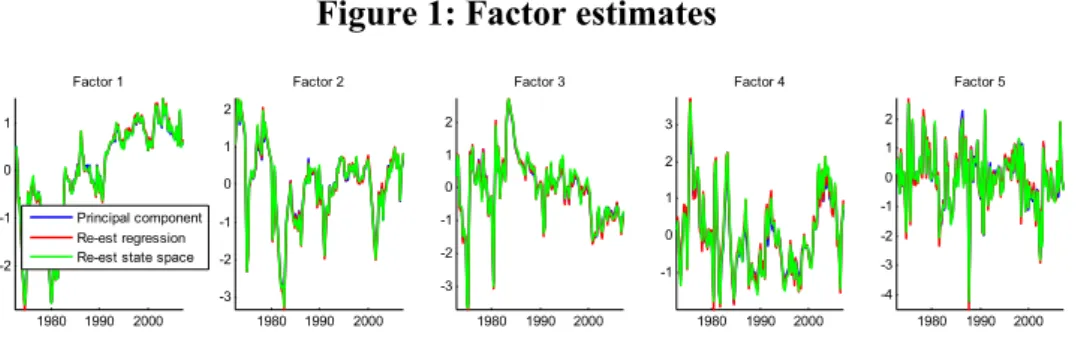
Figure 1 shows the estimated factor paths. To assess whether the PC approach is adequate for estimating factors in the presence of time variation in the factor loadings, we derive an
alternative factor estimate from a cross-sectional regression of the Q variables {l>w on the
estimated time-varying loadingsˆl>w|W, for each period w. The estimated factors resulting
from this exercise (displayed in the same figure in red) show a strong similarity to those
estimated from the PC analysis, the respective correlation coe!cients all exceed 0.99.
In addition, we can also run a full filtering exercise, treating our estimated parameter paths as fixed, now treating the factors as unobservable states, and then using the Kalman smoother to re-estimate them. For this exercise, the transition equation of the resulting
state space model is: Ã Iw Iw31 ! = Ã ˆ Sw3|W1Kˆ1>w|W Sˆw3|W1Kˆ2>w|W LJ 0J ! + Ã Iw31 Iw32 ! + Ã LJ 0J ! ˜ xw (4.1) withH(˜xw) = 0> H(˜xwx˜w0) = ˆSw3|W1VˆwSˆ 310 w|W
and the measurement equation is
[w= h ˆ w|W>0Q×J i à Iw Iw31 ! + ˜hw> (4.2)
where objects with hats and subscript w|W denote the parameter paths estimated in the
first step, in which the factors had been kept fixed at their PC estimates.7 Running the
Kalman smoother on the state space model (4.1)-(4.2) delivers factor estimates that are likewise very close to the PC estimates, and accordingly also close to the factors obtained from the cross-section regression.
Overall, this exercise provides (heuristic) support for our assumption to keep PC-based factor estimates fixed when estimating the time-varying parameters.
4.2
Time variation in parameters and volatility
One may wonder whether a constant-parameter specification would su!ce or whether
time variation in the parameters is really needed and, if yes, which sources of parameter variation are most important. One way to quantify the overall degree of time variation in
the autoregressive matrixKw, the contemporaneous-relations matrix Sw, and the loadings
lw, is to count the number of occasions when the standard deviation of the innovations of
the time-varying parameters — the respective elements ofdiag(T)in (2.7) — are significant.
However, conducting such a multitude of individual significance tests in the usual fashion
may lead to a biased assessment of the overall degree of time variation.8 Moreover, a
further complication arises as under the null hypothesis of no variation, the respective parameter lies on the boundary of the allowable parameter space. Accordingly, we resort to a more direct approach of gauging the overall degree of time variation in the system: we count the number of parameters, for which the time evolution estimated by the Kalman smoother is ‘a straight line’, i.e for which the standard deviation of the smoothed parameter series is essentially zero.
7
The ‘dual’ state space representation (4.1)-(4.2) of a time-varying FAVAR is only valid if the idio-syncratic components in (2.6) are serially uncorrelated, i.e. l = 0 for alll. In the relevant case with autocorrelated idiosyncratic errors the idiosyncratic components would enter the state vector which would be of dimension2J+Q instead of2Jas in (4.2). We abstain from conducting the exercise with this large (346)-dimensional state vector, but instead use the mis-specified state space representation (4.1)-(4.2), where we ignore the autoregressive structure of the measurement error in (4.2).
8
If these tests are conducted with an eective size of, say, 5%, then even in the extreme case of no time variation at all, one would expect to reject the null hypothesis of no time variation 5% of the time.
It turns out that there is actual time variation (i.e. no ‘straight-line’ parameter paths)
for: 6 out of the 50 parameters of theKautoregressive matrix (containing the dynamics of
the VAR(2) for the 5 factors); 1 out of the 10 (= 0=5·5·4) parameters of theS matrix of
contemporaneous relationships of the VAR; and 845 out of the 1680 loadings (since there are 5 loadings, one for each factor, for each of the 336 variables).
Finally, we have assessed whether there is indeed time variation in the volatilies of the
shocks, i.e. whether the elements ofej in equation (2.8) are significant. The corresponding
t-statistics are based on the estimated standard errors which are obtained from the negative inverse of the Hessian of the likelihood function. We find that 5 out of 25 parameters are indeed significant at the 5% level, 2 more parameters are significant at the 10% level.
In summary, the results in this section based on our estimated TV-FAVAR indicate that most of the time variation in the behaviour of US macroeconomic and financial variables over 1972-2007 is associated with changes in the impact of the factors on the variables under analysis and with changes in the volatility of the shocks (which is linked to lagged factors in our model). The degree of variation in the contemporaneous or dynamic relationships across factors is more subdued.
4.3
Diagnostic checking
We first want to check the adequacy of the chosen VAR lag length. If longer lags were needed, the estimated residuals would be correlated over time. Hence, in Figure 2 we report the estimated autocorrelation function (ACF) for the standardized VAR residuals, together with asymptotic 95% confidence bands. Overall, Figure 2 does not provide any major evidence against the assumption of no correlation of the VAR(2) errors.
Similarly, one may wonder whether our assumption of AR(1) idiosyncratic components,
while standard in the literature, is su!cient to clean from temporal correlation. Formal
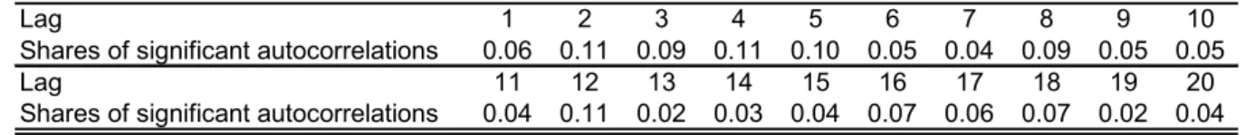
statistical testing is complicated since the joint null hypothesis has a large number of components. To provide at least some indication of the existence of possible problems, in Table 1 we report the percentage of the 336 idiosyncratic residuals (one for each of the variables under analysis) for which a given lag of the ACF is outside the asymptotic bands. For example, only 6 percent of the residuals have the first lag of the ACF outside the bands. Hence, this informal diagnostic check does not provide evidence against our assumption of AR(1) idiosyncratic components.
5
Forecasting with the TV-FAVAR
In this section we evaluate the forecasting performance of our proposed TV-FAVAR ap-proach for a set of key variables. We predict variables representing real activity (including growth of GDP, consumption, investment, industrial production, employment as well as
the unemployment rate and capacity utilization), inflation (changes of the GDP deflator, the CPI, the personal consumption deflator, the PPI, and unit labor costs), and a number of financial and monetary variables.
The factors are estimated as the first J = 5 PCs of our dataset, and they are then
modeled together with each target variable as a time-varying VAR whose parameters evolve as independent random walks. The TV-FAVAR forecasting model thus includes overall 6 endogenous variables/factors, and its lag length is, again, set to 2. Hence, for
each variable of interest {l>w, we have |l>w:= (Iw> {l>w), with
|l>w=D1>l>w|l>w31+D2>l>w|l>w32+yl>w> (5.1)
where each element of D1>l>w and D2>l>w evolves as an independent random walk and the
volatility of yl>w is modeled as in (2.8).9 Note that with respect to the TV-FAVAR
speci-fication in section 2, the forecasting model allows for a feedback from the target variable
to the factors, and for a direct eect of past values of the target variable on its current
evolution. Both features are fairly standard in forecasting models and represent a direct extension of the TV-FAVAR from section 2.
5.1
In-sample forecasts
We first conduct an in-sample forecast exercise for the whole sample period. Given
smoothed estimates ofD1>l>wandD2>l>w for some timew, forecasts for horizons of one to four
quarters are computed as the conditional expectations implied by the associated VAR. In-sample evaluation is fairly common in the literature on the forecasting performance of time-varying models, see e.g. Stock and Watson (2008).
In addition to the full sample forecast evaluation, we also assess how well the TV-FAVAR predicts each variable when it goes through recessions, which has proven
par-ticularly di!cult with constant-parameter models. The recessionary periods are defined
according to the NBER chronology. Moreover, the forecast evaluation is also separately applied for the subsample 1995-2007, since there is evidence of a worsening in the perfor-mance of several forecasting methods (relative to naive predictors) over the more recent years, see e.g. D’Agostino et al. (2007).
We take an AR model as the benchmark and compare its root mean squared forecast error (RMSE) with RMSEs resulting from a FAVAR with constant parameters, an AR with time-varying (random walk) parameters, the TV-FAVAR assuming constant volatility, and the full TV-FAVAR. This exercise allows us to assess whether there are gains not only from using a large information set as summarized by the estimated factors, but also from moving from a constant to a time-varying parameter setup, and from explicitly modeling volatility.
9
We take the five lagged latent factors as volatility regressors in the first five equations. The last equation’s volatility features these factors as well, but in addition the lagged variable of interest.
For comparability, we set the lag length of the benchmark AR model, the TV-AR, the constant-parameter FAVAR and the TV-FAVAR with constant volatility also to 2.
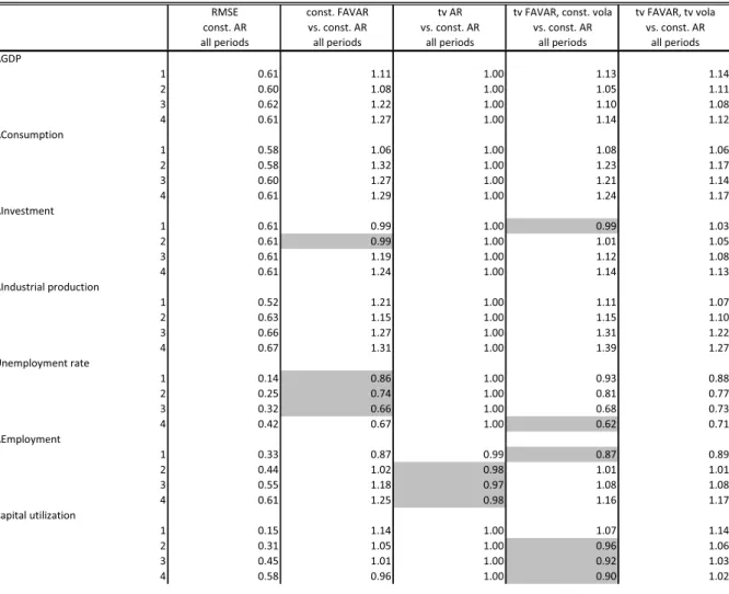
The three panels of Table 2 report the results for, respectively, the real activity, inflation and interest rate and monetary, credit and asset price variables. Each panel contains five
groups of results. The first group reports the RMSEs resulting from the benchmark
constant-parameter AR model. The second to fifth groups contain relative RMSEs of the constant-parameter FAVAR, the TV-AR and the TV-FAVARs without and with changing volatility vis-à-vis the benchmark AR.
Each group has three columns, referring to the full sample, the sample containing recessions only, and the sample as of 1995, respectively. Shaded areas indicate the smallest value for the respective evaluation period (full, since 1995, recessions), if the respective relative RMSE is smaller than 1. Otherwise, i.e. when no model beats the constant-parameter AR, no result is shaded.
It turns out that the constant-parameter FAVAR generally outperforms the AR model, suggesting that there are gains from exploiting information from a large number of vari-ables. For most variables, gains from using a FAVAR compared to an AR model are larger during recessions than over the entire sample period (including both recessions and expansions). This pattern seems to be due to the marked increase of the RMSE of the benchmark AR model during recessions. However, the relative performance of the FAVAR tends to deteriorate substantially after 1995, in line with previous studies.
The performance of the TV-AR is in general very similar to that of the benchmark. In fact, for some variables, where the ML estimates of parameter innovation variances are ‘small’, the Kalman smoother essentially estimates the (potentially) time-varying para-meters as constant and sets them equal to their counterparts from the constant AR(2) — in turn generating the same forecasts. There are some gains for a few variables, such as employment growth and CPI inflation, and some large losses for the Federal Funds rate. Thus, the constant-parameter AR cannot be improved much by allowing time variation in the same univariate model, but rather by using a a large information set as in the constant-parameter FAVAR.
On average over the whole sample period, the TV-FAVAR outperforms the FAVAR with constant parameters for a vast majority of the considered variables and horizons. Over the whole evaluation sample, keeping the volatility of the FAVAR constant in general helps for real activity and inflation variables, but not for financial indicators. Time-varying volatility seems to matter even more after 1995. Over this more recent period, the gains with respect to the benchmark AR still shrink as for the constant-parameter FAVAR, but in general they remain positive and often sizeable.
Finally, the TV-FAVAR with or without time-varying volatility appears to perform best also during recessions, with large and systematic gains for virtually all variables.
5.2
Out-of-sample forecasts
We complement these results with a pure pseudo out-of-sample assessment, where in each quarter of the evaluation period, which ranges from 1995Q1 to 2007Q2, each model is
re-estimated and forecasts for one to four quarters ahead are computed.10 11 The results are
reported in Table 3, whose structure resembles that of Table 2, but omits the distinction between evaluation periods.
On average, the performance of the TV-FAVAR deteriorates by about 20 percent with respect to the in-sample analysis evaluated over the period since the mid-1990s. Since the behaviour of the benchmark is virtually the same, such a deterioration is due to the use of the filtered rather than the smoothed parameter estimates for the TV-FAVAR, and possibly also due to undesirable swings in hyperparameters.
The gains with respect to the constant-parameter FAVAR also shrink. Besides the mentioned estimation issue with the TV-FAVAR, a second reason for this finding is that recursive estimation of the constant-parameter FAVAR introduces by itself a form of pa-rameter time variation, which is instead absent in the in-sample analysis. Of course, the improved forecasting performance of the constant-parameter FAVAR when recursively es-timated is at odds with the underlying assumption of parameter stability, making the resulting estimators biased and inconsistent, though more useful for forecasting.
Notwithstanding the mentioned problems, the TV-FAVAR with constant or changing volatility still works reasonably well for some variables such as capacity utilization, CPI inflation, changes in unit labor costs, and several financial indicators, e.g., changes in loans and in house prices.
In summary, the results suggest that there are gains from both exploiting a large information set and modeling time variation in the parameters. The in-sample analysis indicates that the TV-FAVAR gains remain when forecasting during recessions, which is often complex and problematic, and also in the post-1995 period, when typically standard constant-parameter factor models do not perform so well. For the latter result, allowing for changes in volatility is important. Finally, when forecasting in the post-1995 period in an out-of-sample context, the performance of the TV-FAVAR deteriorates by about 20 percent, mostly due to higher estimation uncertainty, while that of the constant-parameter FAVAR improves in relative terms, due to recursive estimation, which introduces a form of parameter time variation. However, the TV-FAVAR still produces the best forecasts for a few inflation variables and for several financial indicators.
1 0
The estimation window is expanded quarter by quarter. The first estimation window reaches until 1994Q1.
1 1
6
Structural analysis
In this section we examine how the transmission of monetary policy in the US has changed over time. We first discuss why changes in the transmission mechanism of monetary policy may have occurred over the sample period and provide an overview of the existing empirical evidence. We then present new evidence based on our TV-FAVAR. We explain how we estimate the latent factors in the structural setting, how we identify monetary policy shocks, and how we compute impulse response functions and standard errors around them. Finally, we provide evidence on the time variation in the volatility of monetary policy shocks and assess the evolution in the transmission of monetary policy shocks.
6.1
Existing empirical evidence and possible reasons for changes in the
monetary transmission mechanism
The monetary transmission mechanism in the US may have changed over the period under investigation (1972-2007) as a consequence of several structural changes which comprise three major aspects. First, there was some variation in the conduct and strategy of mon-etary policy in the late-1970s/early-1980s with a greater emphasis on price stability and, hence, a better anchoring of long-run inflation expectations, see Boivin and Giannoni (2002) and Galvao and Marcellino (2010) for evidence. Second, liberalization and inno-vation in financial markets is certainly relevant, which also mostly occured in the late
1970s/early 1980s.12 Third, globalization, i.e. greater trade and financial openness, may
have resulted in capital market interest rates being increasingly determined by global de-velopments, see e.g. Boivin and Giannoni (2010), rather than by domestic forces such as monetary policy.
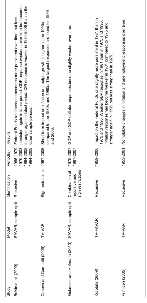
Despite numerous studies on this topic, the empirical literature is still lacking a consen-sus on how the transmission of monetary policy shocks in the US has changed over time. Table 4 overviews recent time-series work on monetary transmission on inflation and
activ-ity. The evidence is based on a variety of methods which dier in the way time-variation
in the parameters is modeled (split-sample versus smooth parameter changes), in the way monetary policy shocks are identified (recursive identification versus sign restrictions), and in the amount of information exploited (small-scale VARs which use a handful variables versus FAVARs which exploit hundreds of variables). VAR-based papers generally focus
on the eect of monetary policy on a single measure of real activity and a single inflation
1 2
On the one side, it subsumes the phasing out of regulation Q and the growth of securitization which may have weakened the balance sheet and bank capital channels and, hence, the transmission of monetary policy to the economy. On the other side, financial market liberalization and innovation comprise the introduction of risk-oriented capital adequacy requirements, the creation of an interstate banking system, the promotion of fair-value accounting and the democratization of credit, which may have strengthened the balance sheet channel. See Boivin et al. (forthcoming).
measure whereas FAVAR-based analyses assess a wider spectrum of activity, inflation but also financial measures. The table shows that the evidence on how the transmission of monetary policy shocks on output and inflation has changed is inconclusive ranging e.g. for inflation from a decline in the transmission over time, e.g. Boivin, Giannoni, and Mi-hov (2009), over no change, e.g. Primiceri (2005), to an increase (e.g. Baumeister et al. (2010).
Despite of inconclusive results regarding the transmission of monetary policy shocks there exists, however, a broad consensus that monetary policy shocks have been large in the early 1980s during the Volcker disinflation and have become smaller since then, e.g. Boivin and Giannoni (2002), Eickmeier and Hofmann (2010), Primiceri (2005), Canova and Gambetti (2009).
In addition to the above mentioned structural changes that have occurred either rel-atively quickly (in the case of institutional changes or changes in the conduct of policy)
or gradually (in the case of globalization) and probably have permanent eects on the
monetary transmission mechanism, economic frictions may lead to asymmetric responses of the economy to monetary policy shocks over the business cycle. Peersman and Smets (2002), for instance, show for the euro area that monetary policy shocks have a stronger
eect on output and prices in recessions than in booms. Results for the US are missing to
our knowledge.
While it would certainly be very interesting to shed light on all these possible changes, we need to restrict ourselves in this application of our TV-FAVAR. We focus on changes in the transmission to activity, prices, inflation expectations and long-term interest rates, thus tackling the first and third types of permanent structural changes as well as the asymmetry question mentioned above, and we leave changes related to financial markets to future research.
6.2
Monetary policy shock identification
For the structural analysis, it is now assumed that [w is driven by a (J+ 1)×1-vector
consisting ofJlatent factorsIW
w and the Federal Funds ratelwas the(J+ 1)th observable
factor as in Bernanke et al. (2005). We will use J = 5 factors. We estimate the space
spanned by the factors using the firstJ+ 1PCs of the data[w. To remove the observable
factor from the space spanned by all J+ 1factors we split our dataset into slow-moving
variables, i.e. variables that are expected to move with delay after an interest rate shock, and fast-moving variables, i.e. variables that move instantaneously in response to an interest rate shock. The slow-moving variables comprise, e.g., real activity measures, consumer and producer prices, deflators of GDP and its components and wages, whereas the fast-moving variables are financial variables such as asset prices, interest rates or
the set of slow-moving variables, denoted byIbwvorz. We then carry out a multiple regression
of Iw on Ibwvorz and on lw, i.e.
Iw=dIbwvorz+elw+w=
An estimate of IW
w is then given by ˆdIbwvorz. In the joint factor vector Iw [ ˆIwW> lw], the
Federal Funds rate lw is ordered last. Given this ordering, the VAR representation of our
(TV-)VAR with lower-triangular contemporaneous-relation matrix Sw directly identifies
the monetary policy shock as the last element of the innovation vector xwin (2.5). Hence,
the shock identification works via a Cholesky decomposition, which is here readily given
by the lower triangularSw3|W1.
The methodology also allows for other identification approaches, such as sign restric-tions which need to be satisfied at each point in time. We have checked that, based on our Cholesky identification scheme, non-borrowed reserves and monetary aggregates decline after an unexpected monetary policy tightening at all points in time. Hence, our results are consistent with the sign restrictions imposed, e.g., in Uhlig (2005) and Benati and Mumtaz (2007), and also with the 1979-1982 period when the Federal Reserve temporarily targeted non-borrowed reserves as opposed to the Federal Funds rate.
6.3
Computing time-varying impulse responses
The impulse responses are based on the assumption that the system (shock propagation)
remains at its time w estimate from time w henceforth. This is common practice and
consistent with our assumption of random walk parameter evolution. 13
That is, at time w, we compute impulse responses in the usual fashion from the
esti-mated VAR
Iw = Sw|W31K1>w|WIw31+= = =+Sw|W31Ks>w|WIw3s+zw>
H(zwzw0) = Sw3|W1VˆwS
310
w|W >
in conjunction with the estimated loading equations
{l>w=0l>w|WIw+ ˜hl>w=
Confidence bands for the impulse response functions at time w are computed as
fol-lows. Recall that we have obtained from the Kalman smoother the estimates of the states
1 3
More specifically, for computing the eect of the shock at timew, one takes conditional expectations also on the future evolution of parameters, where the information set at timewcontains the best (smoothed) estimate of the model parameters at that point. Given the random walk assumption of parameters and the assumed independence of parameter innovations from factor innovations, it is straightforward to see that impulse responses (dierence of conditional expectations of variables atw+kwith and without shock) can be computed as in constant-parameter VARs, replacing the constant parameters by the time-westimates of time-varying parameters. As an alternative (not chosen here), one may take the view that we actually know how shock propagation has changed after time w, so one may condition on the (estimated) future evolution of system parameters when computing the response to the shock.
djw|W (containing the respective elements of the rows of S and K), and the
correspond-ing variance-covariance matrices jw|W for each VAR equationj = 1> ===> J+ 1. Moreover,
we have for the loading equations the smoothed ˆl>w|W with the corresponding
variance-covariance matricesYl>w|W. We generate draws of j> j = 1> ===> J+ 1fromQ(djw|W>
j w|W). If
the VAR matrices implied by the set of draws satisfy the non-explosiveness condition, we keep the draw, otherwise we discard it and repeat the previous step. We draw until we
have gatheredN= 1000successful draws. We then drawNtimeslfromQ( ˆl>w|W> Yl>w|W).
For a given timew, variableland horizonk, the desired quantiles of the impulse response
function are then obtained from the Ndraws. A caveat of this approach is that we ignore
the uncertainty associated with the estimation of the hyperparameters.
6.4
Monetary policy shocks and transmission in our TV-FAVAR
We have reported in section 4 to what extent the volatility estimates of the VAR inno-vations to unidentified factors were varying over time. Figure 3 now shows the estimated volatility of the monetary policy shock. Consistent with the literature, the volatility peaks in the early-1980s which is generally labeled the ‘Volcker disinflation’ and declines there-after. We also observe a peak around 1974. One explanation might be that, possibly due
to overestimation of the negative eects on activity of the oil embargo in October 1973,
the output gap was substantially underestimated and, hence, the Federal Funds rate was much lower than that implied by a simple Taylor rule, see Orphanides (2003). We find indeed a large sequence of expansionary monetary policy shocks around 1974 (not shown) and heightened volatility of the shocks which might reflect this mis-perception.
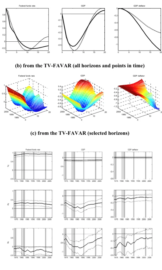
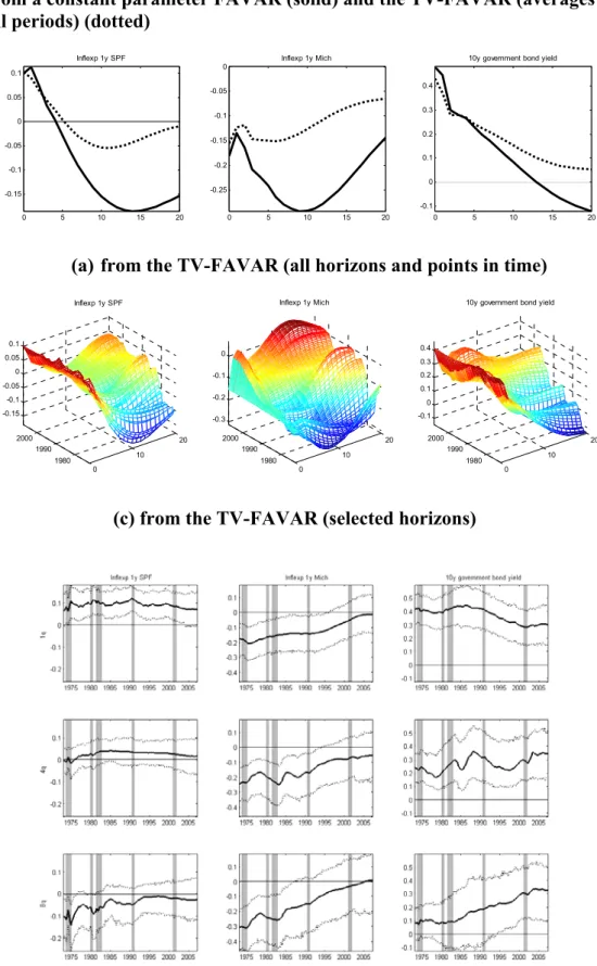
Based on the TV-FAVAR and the described identification scheme we now assess the evolution of selected impulse response functions to a monetary policy shock over time. We focus on three questions. (i) Has the transmission to key macroeconomic variables changed over time and, if yes, how? (ii) Can we detect asymmetries in the monetary transmission, and, more specifically, are monetary policy shocks transmitted to economic activity more strongly during recessions than during booms? (iii) Has the transmission to inflation expectations and long-term interest rates changed over time and, if yes, how?
Figures 4, 5 and 6 show impulse response functions of three key macroeconomic vari-ables (the Federal Funds rate, GDP, and the GDP deflator), of additional activity and price variables (consumption, investment, industrial production, employment, GDP defla-tor, PPI finished goods, the PCE defladefla-tor, unit labor costs), of two inflation expectation measures (taken from the Survey of Professional Forecasters (SPF) and the survey con-ducted by the university of Michigan) and the 10-year government bond rate, respectively. To focus on transmission only, we show estimates of impulse response functions to a mon-etary policy shock which raises the Federal Funds rate on impact by 1 percentage point. Panels (a) show averages of point estimates of impulse responses over the entire sample