Poi-icY
RESEARCH
WORKING
PAPER
1942
Poverty Correlates
and
Social
protection
systems
in
the transition economies have
Indicator-Based Targeting
been inadequate to meet thein Eastern Europe and the
challenges of transition, beingboth costly and poorly
Former
Soviet Union
targeted. The largest group ofpoor people is the working poor - especially workers
Christiaan Grootaert with little education (primary
Jeanine Braithwaite education or less) or outdated
vocational or technical education.
The World Bank
Social Development Department and
Europe and Central Asia
Poverty Reduction and Economic Management Sector Unit July 1998
Public Disclosure Authorized
Public Disclosure Authorized
Public Disclosure Authorized
| POLICY RESEARCH WORKING PAPER 1942
Summary findings
Grootaert and Braithwaite compare poverty in three social transfers (other than pensions) or other nonearned Eastern European countries (Bulgaria, Hungary, and income. But through sheer mass, the largest group of Poland) with poverty in three countries of the former poor people is the working poor - especially workers Soviet Union (Estonia, Kyrgyz Republic, and Russia). with little education (primary education or less) or They find striking differences between the post-Soviet outdated vocational or technical education. Only those and Eastern European experiences with poverty and with special skills or university education escape poverty
targeting. Among patterns detected: in great numbers, thanks to the demand for their skills d Poverty in Eastern Europe is significantly lower than from the newly emerging private sector.
in former Soviet Union countries. * The poverty gap is remarkably uniform in Eastern * Rural poverty is greater than urban poverty. European countries, especially Hungary and Poland, * In Eastern Europe there is a strong correlation suggesting that social safety nets have prevented the between poverty incidence and the number of children in emergence of deep pockets of poverty. This is much less a household; in the former Soviet Union countries this is true in the former Soviet Union, where those with the less pronounced, except in Russia. highest poverty rate also have the largest poverty gap. * There is a gender and age dimension to poverty in In the short to medium term, creating employment in some countries. In single-person households, especially the informal sector will generate a larger payoff than of elderly women, the poverty rate is very high (except in creating jobs in the formal (still to be privatized) sector, Poland) and poverty is more severe. The same is true in so programs to help (prospective) entrepreneurs should pensioner households (except in Poland). In Poland the take center stage in poverty alleviation programs. pension system has adequate reach.
* Poverty rates are highest among people who have lost their connection with the labor market and live on
This paper is a joint product of the Social Development Department and Europe and Central Asia, Poverty Reduction and Economic Management Sector Unit. The study was funded by the Bank's Research Support Budget under the research project "Poverty and Targeting of Social Assistance in Eastern Europe and the Former Soviet Union" (RPO 680-33). Copies of this paper are available free from the World Bank, 1818 H Street NW, Washington, DC 20433. Please contact Gracie Ochieng, room MC5-158, telephone 202-473-1123, fax 202-522-3247, Internet address [email protected]. The authors may be contacted at [email protected] or [email protected]. July 1998. (112 pages)
Poverty Correlates and Indicator-Based
Targeting in Eastern Europe
and the Former Soviet Union
Christiaan Grootaert Jeanine Braithwaite
The authors would like to thank RobertAckland, Branko Milanovic, and Gi-Taik Oh for comments on an earlier draft, and Precy Lizarondo and Gracie Ochieng for document processing.
Table of Contents
Page
1. INTRODUCTION ... 12. METHODOLOGICAL ISSUES IN THE MODELING OF POVERTY .. 3
3. POVERTY PROFLES .. 20
A. Eastern Europe .23 Location .25
Family Composition .26 Labor Force Participation .30
Gender and Age .36
B. Former Soviet Union .41
I. Pre-Transition Poverty and Macroeconomic Impact of Transition .42
II. Who are the Poor After Five Years of Transition? . 44
Location .45
Family Composition .'46 Labor Force Participation .50 Gender and Children .54
4. MULTIVARIATE ANALYSIS OF WELFARE AND POVERTY.. 54
A. Eastern Europe 56
Welfare Equations .56 Poverty Equations .62 Poverty Gap Equations .66 B. Former Soviet Union .70
Welfare Equations .70 Poverty Equations .76 Poverty Gap Equations .81
6. S U ... MMARY 99
REFERENCES ... 106
1. Introduction
This paper undertakes a comparative analysis of poverty in three East European countries (Bulgaria, Hungary, Poland,) and three countries of the Former Soviet Union (FSU) (Estonia, Kyrgyz Republic, Russia). To that effect, we constructed a comparative data set, whereby household survey data from the six countries were carefully checked, cleaned and made comparable. The resulting data set has been dubbed HEIDE (Household Expenditure and Income Data for Transitional Economies) and its content and construction method are described in detail in Ackland et al (1997).
Although our analysis of the HEIDE data found elements in common, the most striking result is how different the post-Soviet experience with poverty and targeting is from the East European one. Overcoming the Soviet legacy has not been as easy as the generally positive East European prototypes would have suggested. Poverty correlates for the FSU are not as sharp nor as well-defined as in Eastern Europe, yet poverty levels are also higher in the FSU, presenting a larger challenge to governments as they try to reduce poverty and improve targeting.
We have set ourselves three tasks in this paper. First, we construct a profile of the incidence and depth of poverty in the six countries, using aggregate poverty indexes. The aim is to find out what the common elements are in the profile of poverty in Eastern
Europe). If we find a large common element, it opens up the possibility of a region-wide
policy approach to poverty alleviation.
Second, we undertake a multivariate analysis of the determinants of poverty. This
overcomes the limitations of the one- or two-dimensional approach typically embodied in
a tabular presentation of a poverty profile. The econometric modeling work addresses
separately the incidence of poverty and the depth of poverty, using reduced-form
equations. Our objective is to find important correlates of poverty, and, where possible,
attribute causality to them. The results will also clarify whether the determinants of
welfare, such as the demographic characteristics of households and the returns to
household assets, differ between the poor and the non-poor.
Our third and most important task, is to derive a policy approach towards poverty
alleviation. Specifically, we wish to evaluate the role which means testing and
indicator-based targeting can play in channeling social transfers to the poor. In part because of the
socialist legacy, social transfers constitute a huge component of public expenditure in
Eastern Europe and the FSU, representing as much as one-fifth of gross domestic product
(GDP). The need to reduce these expenditures is pressing and the need for suitable
targeting devices is high. We will demonstrate the contribution which indicator-based
targeting can play.
Each of these three tasks is given a section in this paper (respectively, sections 3,
4, and 5). Before presenting empirical results though, we address in the next section the
2. Methodological Issues in the Modeling of Poverty
In line with most recent work on poverty, the analysis in this paper is based on a
money-metric measure of utility and welfare. Total household expenditure is used as measure of household welfare and as a basis to rank households and to define a poverty line. Expenditure is preferred to income because it is usually better reported in household budget surveys.' Furthermore, there is the important theoretical consideration that expenditure reflects better permanent income. This argument is particularly relevant in transition economies where the volatility of current income is still quite high, due to the lack of steady private sector employment and the resulting high rates of unemployment. Arrears on the payment of wages and pensions, especially in FSU countries, further adds to the unreliability of current income as a measure of welfare.
The analysis below takes into account differences in needs due to different household size and composition and therefore uses household expenditure per equivalent
adult as the welfare measure. There is a wide choice of adult equivalency scales, and different scales are used in different countries. Our comparative analysis objectives
require the use of a single scale, and we have opted for the OECD scale, because of its simplicity of use and wide familiarity. This scale is expressed as follows
EPEQ = (0.7)
where EXP is total household expenditure and n is household size.2 The OECD scale reflects economies of scale due to household size but does not incorporate gender differences.
Household expenditures were not deflated by a regional price index to take potential differences in prices within the country into account. The reason is that, except for Russia, the countries in the analysis are all fairly small and regional price differences
can be expected to be minor. For example, for Poland (the second largest country in the set), regional price differences were found not to exceed 2 percent (Grootaert, 1995). For Russia, informal calculations suggested that the effect on poverty estimates of corretting for regional price differences was very small. During the period of analysis, several
countries experienced significant inflation and in these cases expenditures were deflated with a month-by-month consumer price index. This yields real household expenditure per
equivalent adult as measure of household welfare.
A cut-off point needs to be selected to serve as poverty line across the distribution of real household expenditure per equivalent adult. We rejected the use of an absolute line, such as x dollars in PPP-terms, due to the wide variation in income levels across the six countries. Indeed, it is not very meaningful to compare poverty profiles, when for one country the profile pertains to less than 5 percent of the population and for another
2 For the household sizes typically found in Eastern Europe and the FSU, this fonnulation is a close equivalent of the more conventional statement of the OECD scale whereby the first adult = 1, other adults = 0.7, and children = 0.5. The exponential formulation however simplifies the calculations.
country to almost half the population. Hence, we opted for a relative poverty line, which
after some experimentation, was set at two thirds of mean household expenditure per
equivalent adult.3
Obviously, the exact position of the poverty line selected affects the results. Individual country studies have shown that in certain ranges of the distribution, even fairly
small movements of the poverty line can have large effects on the estimated incidence of poverty (see e.g. Grootaert, 1995 for Poland; Grootaert, 1997a for Hungary; World Bank, 1995b for Russia). -However, poverty profiles tend to be more robust than incidence
figures, and significant modifications do not tend to occur unless the poverty line is set in
the very lowest ranges of the distribution, especially in the lowest decile. Nevertheless, a sensitivity analysis would be useful, and the earlier cited country studies contain analyses
with different poverty lines. The sheer bulk of tabular and regression results for a
six-country study make it impractical however to include a formal sensitivity analysis in this
paper. We refer the interested reader to the country studies.
Our selection of aggregate poverty index is the popular P-alpha class of poverty
measures introduced by Foster, Greer and Thorbecke (1984). This index is defined as
q
where n = number of people q = number of poor people z = poverty line
yi = expenditure of individual i a = poverty aversion parameter
The poverty aversion parameter can take any positive value or zero. The higher
the value the more the index "weighs" the situation of the very poor, i.e., the people farthest below the poverty line. Of specific interest are the cases where a = o and a = 1.
If a = o, the index becomes
p =q n
which is the simple head count ratio of poverty, i.e. the number of poor people as a
percentage of the total population. While this is a useful first indicator, it fails to pay
attention to the depth of poverty. To do so, one also needs to look at the extent to which
the expenditures of poor people fall below the poverty line. This is customarily expressed as the "income gap ratio" or "expenditure gap ratio" which expresses the average shortfall
as a fraction of the poverty line itself, i.e.,
z-y' z
A useful index is obtained when the head count ratio of poverty is multiplied with the income or expenditure gap ratio. This corresponds to
which reflects both the incidence and depth of poverty. This measure has a particularly useful interpretation because it indicates what fraction of the poverty line would have to be contributed by every individual to eradicate poverty through transfers, under the assumption of perfect targeting. This can be considered as the minimum amount of resources needed to eradicate poverty, given that perfect targeting is not likely to be achieved in practice.
In the tables below we show the head-count ratio Po, and the ratio PI/Po, i.e. the expenditure gap ratio.4 We prefer to call the latter "poverty gap" (PG) to highlight that it
is a measure of the average depth of poverty calculated over the poor only. In contrast, Po and Pi are ratios which are calculated over the entire population (for a further discussion of these measures, see Ravallion, 1993). In the tables below each of these measures has been multiplied by 100 for easier interpretation.
The comparative poverty profile in the next section of this paper is based on one-or two-dimensional disaggregations of the P-alpha index. While this yields a useful
identification of important correlates of poverty, it cannot establish the relative importance of each correlate (or determinant, if causality can be assumed). A multivariate model of poverty is hence indicated. A basic model uses real household expenditure per equivalent adult as dependent variable in a regression with exogenous household endowments and characteristics as explanatory variables. Such welfare model is a reduced-form equation of the various structural equations which express the income-earning and consumption behavior of the household (see e.g. Glewwe, 1991). This model can explicitly recognize the economic characteristics of the environment in which households operate. Consider the following model:
E, =/3X, +82W + s, (1)
where Ei = real household expenditure per equivalent adult of household i
Xi = a set of characteristics of households i
Wi = a set of characteristics of the economic environment of household i
A,2 = model parameters
-aj = error term
While such model is not able to predict the effect of household characteristics on specific income or consumption decisions (this would require structural equations), it allows to observe the net effect of any given characteristic, holding all others constant, on resulting household welfare. It is assumed at this point that there is no simultaneous effect of household welfare on household characteristics so that no X, are endogenous. This assumption is time-dependent, i.e., we assume this to be the case within some relevant time period. (We revisit this issue below when discussing the specific variables to be
included in the model). With this assumption, simple OLS estimation of equation (1) is appropriate.
From the point of view of understanding poverty, equation (1) is not necessarily optimal. It unposes constant parameters over the entire distribution. It thus assumes that the effect of a given household characteristic, e.g. education, is the same across the entire welfare spectrum, and that the underlying structural equations do not differ for poor and non-poor. One could say that-in this representation the poor are viewed merely as "rich people with less money." This is arguably an incomplete representation. While one should of course not see the poverty line as a barrier which divides the population into two entirely different groups, it is certainly arguable that poor people face different (often more severe) constraints, e.g. to obtain credit, to obtain labor market information, to set up enterprises, etc. On the other hand, they may well be more adept at obtaining transfer income. This calls for additional modeling of poverty.
There are several ways of addressing a situation whereby parameters can be expected to differ across different segments of the distribution. One can estimate the welfare regression separately for poor and non-poor, or introduce a set of interaction variables (between a binary variable for poor/non-poor and the other right-hand side (RHS) variables). Both methods are equivalent econometrically, but their estimation is problematic. In the first method, each group (the poor and the non-poor) forms a
variable. This endogeneity problem also rules out the use of a Heckman-type selection model to, first, determine poverty status and, then, using the derived inverse Mills-ratio to correct the welfare equations of the poor and non-poor groups. In practice, since the poverty criterion is the same as the dependent variable in the welfare equations, it would be very difficult to place an identifying restriction on the welfare equation.
A workable solution is at hand, however, if the situation can be seen as a censored model, in which case Tobit estimation becomes possible. This requires the assumption that equation (1) is the correct welfare model for the poor and that the same set of explanatory variables determine whether one is poor or not. No assumptions are made about the determinants of welfare of the non-poor (the process and the parameters could or could not be the same). The model sets any expenditure level higher than the poverty line equal to the poverty line, i.e. the data are censored at the poverty line.
E;'= E, if E c<z (2)
E = z otherwise
where z = poverty line, and Ei is determined as in equation (1)
This model allows for the possibility of different parameters for the poor and non-poor and can be estimated consistently if the error terms is assumed to be nornally distributed (Maddala, 1983). Furthermore, a comparison of the estimated parameters of (2) with those of (1) provides a test of whether the parameters of equation (1) do indeed differ between the poor and the non-poor. This is especially relevant for the parameters of asset variables, which measure the returns to these assets, and one can hence test whether,
for example, the returns to education differ between the poor and the non-poor (Appleton,
1995).
Conceptually, this model specification corresponds to modeling the poverty gap, i.e. the poor's expenditure shortfall expressed as a ratio of the poverty line, i.e.
z-E, for Ei sz
z
Whereas this ratio is constrained between 0 and 1, the poverty gap itself is constrained between 0 and z. In practice, it ranges between zero and z minus the lowest E, in the sample, which is what equation (2) depicts.
When estimating poverty models on the basis of household survey data, it needs to be recognized that such data are likely to contain a certain amount of measurement error. If the error is limited to the dependent variable, it does not bias the estimated coefficients (so long as the error is not correlated with any of the RHS variables), but it will affect the variance-covariance matrix. A potential concern though is that the measurement error of household expenditure may rise systematically with the level of expenditure. This increases the probability of correlation with RHS variables such as education, which is positively correlated with the level of expenditure. This could lead to biases in the estimation of equations (1) and (2).
poor.5 Diamond et al (1990) estimate a multinomial logit model on U.S. data to predict the probability of belonging to an income quintile, conditional upon certain personal and household characteristics. Diamond et al justify their approach, relative to a continuous
welfare regression, by arguing that the restrictions imposed by the functional form of a levels regression (often linear or log-linear) may cause it to fit poorly on the actual
distribution, and demonstrate that this is the case for their U.S. data set. The multinomial logit model allows for discontinuities in the underlying welfare model and thus also solves
the concern of imposing equal parameters over the entire distribution discussed earlier. In the case of two groups (poor and non-poor) the approach collapses to a binary logit or probit model, although then the underlying welfare model is again continuous (Ravallion, 1996). There has been a recent debate in the literature on the merits of welfare
regressions versus binary poverty models. Ravallion (1996) argues that the binary
response model is redundant, since the parameters measuring the effect of household
characteristics on the probability to be poor can be derived from the levels regression,
which is consistently estimable under weaker assumptions about the distribution of the
error. As argued in Grootaert (1997b), this argument applies if there is only random
measurement error and if a case can be made for imposing constant parameters over the
entire distribution.
As we discussed earlier, the latter issue has been dealt with in this analysis through Tobit estimation of the expenditure of the "poor" segment of the distribution. The
possibility of systematic measurement error has led us to undertake also probit estimation
5 To our Inowledge, the first use of such model in the empirical poverty literature is by Bardhan (1984) in a study of poverty in rural West Bengal.
of a poverty equation where the dependent variable is binary (poor/non-poor). Explanatory variables are the same as in the welfare regression. It is clearly a judgment call whether the loss of information embodied in the binary regression (collapsing the entire distribution into two values) outweighs the risk of bias due to measurement error. However, to the extent that results from a binary model confirm levels-regression results, they can act as- a robustness test for the latter. In recent years, use of probit and logit models (mainly the former) have become common practice in poverty analysis (see e.g. Alderman and Ga7rcia, 1993; Lanjouw and Stem, 1991; World Bank, 1995d, 1996d; Appleton, 1996; Grootaert, 1997b).
In summary, the determinants of poverty will be estimated in this paper on the basis of three models:
(i) OLS regression of welfare equation (1);
To account for differences in parameters between the poor and nonpoor, (the poor are not rich with less money) without losing information from level-regressions:
(ii) Tobit estimation of the welfare level of the poor, based on equation (2); this is equivalent to modeling the poverty gap;
To solve the problem of non-random measurement error (especially mismeasurement as a function of level of expenditure):
Each of these three models has the same RHS and we turn now to the discussion
of which variables can be considered exogenous household characteristics. As we pointed
out earlier, this is mainly a function of the time horizon considered relevant. It has become
fashionable in econometrics to take a rather narrow view on this (i.e., to consider a long
time horizon) and to estimate welfare models with very parsimonious RHS (see e.g.
Glewwe and Hall, 1995). As Appleton (1995) has argued, reasons can be found why
almost every conceivable determinant of poverty is simultaneously determined with
welfare, and he cites a number of examples of such discussions in the literature. In the
end, little more than gender, age and a few parental characteristics end up as truly
6
exogenous. Such econometric purity is problematic if the analysis is meant to guide
policy. Most policy and targeting variables at the household level become endogenous if
the time period is made long enough. All assets (education, physical capital, land) as well
as household size are to some degree a function of the household's welfare level and its
evolution over the life cycle. Location can change due to migration. Likewise, the
household head can change as a result of migration, or the splitting of one household into
several households (or the reverse process).
While we recognize the strict validity of these arguments, for this exercise we have
taken a pragmatic view, and used a fairly generous set of RHS variables. The objective is
to identify determinants of welfare and poverty which, in the short run, are valid policy
and targeting variables. As relevant time frame, we consider the reference period for the
data collection, i.e. a year or less. We include therefore on the RHS variables which the
period or only with great difficulty or cost. This takes the specific situation of these economies into account, and explains e.g. why some labor market variables are included on the RHS. In a filly functioning market economy, occupation and labor market status must be viewed as endogenous, but this is not the case in many transition economies. Unemployment is high and largely structural, retraining opportunities are limited, and in some countries, the supply of housing is not yet sufficiently flexible to permit easy migration to areas of growing labor demand.
On the other hand, among the asset variables, we have not included ownership of durable goods on the RHS for estimating the three models listed above. This is actually more of a judgment call than it may appear. Until a few years ago, in the countries in our analysis, such goods were rationed. With the possible exceptions of Hungary and Estonia, there is not yet a fully operating market for these goods, accessible to the entire population. Markets for durable goods such as personal computers, VCRs, etc. often
exist only in cities, and due to very high relative prices (compared e.g. to Western Europe) accumulation and decumulation of such goods is rare for all but the very rich. For many households, the existing stock is still largely determined by the pre-transition allocation. Nevertheless this situation is rapidly changing.
Generally speaking, asset variables have to be seen as endogenous with respect to household welfare, because in an inter-temporal context, the household's welfare level will
replace these variables with instruments such as parents' education, inherited wealth, etc.
Unfortunately, such variables are not available in the data sets and our regressions include
productive asset variables on the RHS. In interpreting the regression results, some
caution will thus be necessary, not to view the estimated coefficients as measuring strictly
one-way causality from assets to welfare or poverty.
Using a one-year time frame, we consider as exogenous the following sets of variables:
* household assets: education, physical capital (house, household enterprises), land;
o demographic household characteristics: household size and composition and characteristics of the head of household;
* labor market connections: unemployment, and share of wages in total income;
* economic environment: location.
The human capital of the household is embodied in its members and hence their
numbers (by sex and age group) are introduced as regressors. Since it is likely that the
education of the head of household has a greater influence on welfare and poverty
outcomes than that of other members, the education level of the head was introduced as a
separate regressor, by means of a series of dummy variables reflecting the highest level of
education achieved (primary or less, secondary, vocational/technical, university). The
earlier cited country poverty studies have indeed found strong bivariate correlations
between poverty incidence and the level of education of the head of household. The data
The age of the household head is also a good indicator of the stage in the life cycle of the
household.
Information on physical capital is somewhat scant in the data sets. We know
whether the household owns a farm or small business but have no information on the value
of its assets. Nevertheless, information on ownership (or use, in countries where legal ownership is still unclear) is bound to be very important, because the emergence of small private enterprises is a key feature of transition, and poverty among such entrepreneurs is
likely to be below average.
Ownership of a house is important in the same sense. In many cases it provides
the location for a household enterprise, and for many households it constitutes the main asset against which it can borrow and from which it derives rental income (actual or imputed).' In most transition economies, the supply of housing is still quite rigid, and a
housing market is absent in many locations. Housing ownership is still frequently the result of pre-transition allocations by the state. hence, there is a strong case for
considering home ownership as exogenous to the process of determining welfare.
Similarly, ownership of land is in most transition settings not yet a full household choice
variable, and, especially in rural areas, it is a key determinant of cash income and
The link with the labor market is captured in the model with two variables: the share of wages in total household income, and the number of unemployed household members (in some cases this was replaced by the employment status of the head of household, if this variable yielded a better specification). The case for exogeneity of these
variables rests on the fact that in the transition context, many of the labor market status outcomes are determined, or at least greatly influenced, by the labor market status that obtained prior to transition and/or by the macro-economic changes. Of course, it must be recognized that personal characteristics do contribute to unemployment, or make it more
or less likely than a person will successfully obtain self-employment income. Again, instrumental variables would provide a solution if they were available. (E.g. one possibility would be to use regional rather than household-specific labor market variables). We kept these variables in the equation mainly because of their importance for targeting, but again recognize the need for caution in interpreting the coefficients.
The way in which the household utilizes its asset endowment is a function of
various demographic household characteristics. The demographic structure of the
household has been shown to have a strong relation with poverty incidence. Beyond the
number of children and adults, it is useful to specify the age and sex of the household head
because those factors may be related to the household's ability to cope with a changing
economic environment.
Lastly, the incidence of poverty is affected by the economic environment in which
the household operates. This relates especially to income earning opportunities and the level of social and economic infrastructure. In a transition context, the household's ability
to adjust to a new economic reality will depend very much upon whether it lives in an urban or rural area, in a large or small city, in an old industrial region, etc. In this research, we will capture this by categorical variables for type of locality (capital or other
city, village).
Annex 1 shows the means and standard deviations for the full set of variables used
in estimating the welfare and poverty equations.
Apart from laying out the set of determinants of welfare and poverty (the objective
of Section 4), these equations can also be used to investigate how feasible means-testing
and indicator-based targeting is. Almost all East European and FSU countries rely on
these techniques to allocate social assistance and sometimes other transfers as well. If an
effective, reliable and low-cost test for income were available, there would of course be no
need for indicator-based targeting. In practice, most social assistance authorities find it
very difficult to apply means tests and find that applicants on average underreport income,
especially self-employment income. We wanted to test how many poor people could be
correctly identified based on a simplified means test and relying on easily identifiable
indicators. To that effect we re-estimated equation (1) with an expanded set of variables,
adding wage-income and public-transfer income (the two "official" and most easily
verifiable income components for most households), and also a list of durable goods
welfare, but merely as a partial correlation coefficient incorporating all feedback effects from welfare to durable ownership. We estimated the expanded equation (1) with forward step-wise OLS, so as to identify the strongest correlates and best predictors first.8 as to identify the strongest correlates and best predictors first. The results of this exercise are discussed in Section 5.
3. Poverty Profiles
The changing nature of poverty in Eastern Europe and the Former Soviet Union has paralleled the sharp changes in economic management and in government in the region over the past two decades. Even before the collapse of the Berlin Wall and the break-up of the Soviet Union, East European countries had been experimenting with economic reforms which brought their systems closer to market economies. Two of the early leaders in such reform efforts, Hungary and Poland, are case studies for this analysis. Hungary was arguably the first country in Eastern Europe to embrace economic reforms, with its market-oriented New Economic Mechanism, and Poland's Solidarity movement was an early large-scale populist movement towards more democratic government and a freer economic environment.
Along with economic reform in Eastern Europe quickly came the labor market consequences of shutting down non-profitable state enterprises. Unlike in the FSU, where adjustment was much later and fell almost exclusively on real wages, in Eastern Europe,
s It would also be possible to use a step-wise poverty probit equation for this objective. However, most social assistance authorities are interested not just in classifying applicants as poor/non-poor but also in detennining the extent of the welfare shortfall. Hence, the OLS welfare equation is a more useful basis for a predictive model.
open unemployment along with real wage declines was characteristic of phase changes in government and the economy. One paradoxical result of this is that poverty is much more clearly defined in Eastern Europe than in the FSU, and the poverty profiles of East European countries identify poverty correlates more clearly. This makes improvements in targeting in Eastem Europe much more realistic to posit than in the FSU, where the poor
are not so well-differentiated from the not-so-poor.
Although this conclusion might seem somewhat surprising, it is not especially new. Even with far more inferior databases, Atkinson and Micklewright (1992) concluded that poverty in Eastern Europe was more defined and less all-encompassing than poverty in the Former Soviet Union. However, during the reference period for their work (1991 and earlier) the FSU had not broken up; nor had there been the sharp changes in the macroeconomic environment associated with the dissolution of the FSU, so it is not surprising that the earlier time period and the use of official data led Atkinson and Micklewright (1992) to conclude that overall, FSU poverty was not as severe as in many East European countries, but further, that poverty within the FSU was highly heterogeneous (see also Braithwaite, 1991).
With the breakup of the FSU, there were severe disruptions in the old trading and monetary regimes. The demise of the ruble zone, the political ramifications of the declarations of independence, the build-up of arrears in the payment for energy imports,
the aggregate decline in GDP for the East European countries was 10 percent during the
period 1990-96, it was 45 percent for the FSU. Especially sharp declines were registered
in 1993 and 1994, which were run-away hyperinflation years in most FSU countries.
Under these circumstances, it is hardly surprising that open poverty has increased
drastically in the FSU. Poverty also increased in Eastern Europe, but Eastern Europe
managed to avoid most of the macroeconomic disruption associated with the break-up of
the FSU, or if problems such as hyperinflation and collapsing real wages were
encountered, they were encountered much earlier than during 1990-96. As a result,
poverty in Eastern Europe has become much more like poverty in Western
Europe-highly correlated with the situation in the formal labor market and the skills of
individuals. As the poverty profiles below indicate, in the FSU, poverty is not
well-correlated with the nature of labor market participation of household members, but neither
is it -well-correlated with the lack of formal labor market ties. Basically, in the FSU,
poverty is more pervasive than in Eastern Europe and not as well-defined. It is much
more difficult to differentiate a poor FSU household from a non-poor one based on
observable correlates.
These qualitative and quantitative differences in the experience of poverty in
Eastern Europe and the FSU are demonstrated in by the cross-tabulation of poverty
A. Eastern Europe
In Eastern Europe, the start of rapid transition in the early 1990s accelerated the existing trend towards increasing poverty9. The main contributing factors were the loss of employment in a suddenly contracting state-sector, without coincident emergence of private sector employment. Rapidly rising unemployment has in fact been one of the most visible signs of the social costs of transition. A number of East European countries also experienced significant inflation (although it did not reach the level of the hyper-inflation experienced by some FSU countries). Adjustments in wages, pensions and other social transfers lagged behind, and real incomes for many people fell. However, the emerging evidence suggests that these effects have been fairly short-lived. The three East European countries in this study experienced less GDP declines than the three FSU countries, and in the 1994-1995 period, they have each returned to positive growth.
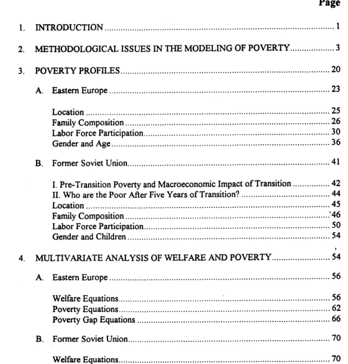
The figures in Table I indicate that poverty rates as well as poverty gaps are lower in the East European countries than in the FSU countries. As a reminder, poverty rates
measure the incidence of poverty as the percentage of population below the poverty line (two-thirds of mean household expenditure per equivalent adult). The poverty gap
measures the depth of poverty as the poor's average shortfall in expenditures from the poverty line expressed as a percentage of the poverty line. (Both measures were discussed
higher (42.5 percent), its poverty gap is lower (25 percent) than Russia's. Hungary and
Poland show the most favorable situation with respective poverty rates of 21 percent and
23 percent. The poverty gap is slightly higher in Hungary (14.1 percent) than in Poland
(13.3 percent). It thus appears that poverty in Eastern Europe is much more shallow than
in FSU, which is good news from the point of view of poverty alleviation in Eastern
Europe. It suggests that as economic growth resumes, rising incomes may rapidly lift
many people above the poverty line.
Table 1: Poverty and Locality
Locality Bulgaria Hungary Poland Estonia Kyrgyz Russia Republic Headcount (P0, in percent) Capital 17.5 20.3 10.1 20.6 22.9 18.2 Other Cities 20.5 17.7 16.9 31.6 38.0 38.4 Urban Subtotal 19.9 18.5 16.2 27.5 33.3 35.8 Rural 39.2 24.0 33.8 38.7 47.2 49.6 Total 26.1 20.6 23.0 30.5 42.5 39.4
Poverty Gap (in percent) 1/
Capital 19.9 13.9 13.4 19.7 24.0 20.7
Other Cities 17.8 13.5 12.7 19.2 26.2 28.7
Urban Subtotal 18.1 13.6 12.7 19.4 25.7 28.1
Rural 21.7 14.6 13.8 21.9 24.7 33.2
Total 19.8 14.1 13.3 20.2 25.0 29.8
Source: Household Expenditure and Income Date for Transition Economies Data Set (HEIDE). Notes: .
1/ The poverty gap is the poor's average shortfall in expenditures from the poverty line, expressed as a percentage of the poverty line (this measure is also known as the expenditure gap ratio).
Location
The strong causal role played by changes in employment in creating poverty during transition in Eastern Europe make it likely that transition economies will show strong geographic patterns of poverty and that urban and rural areas will be affected differentially.
This is confirmed by Table 1 which shows that in all three East European countries rural poverty is higher than urban poverty. In Bulgaria and Poland, rates of rural poverty incidence are almost twice the urban rates. In Hungary, the urban-rural difference is small. Within urban areas, the differences between the capital and other cities are not so pronounced. (This is a marked difference with the situation in the FSU in which capital cities are markedly less poor than other cities). In Bulgaria and Poland, poverty rates are slightly lower in the capital than in other cities, but in Hungary the reverse is true.
The depth of poverty varies less than the incidence of poverty in Eastern Europe. In general, poverty is slightly deeper in rural areas than in urban areas, but within the latter poverty is deepest in the capital cities. So, while East European capitals have generally less poverty than elsewhere, the poor in those capital cities do have a greater shortfall in expenditure than elsewhere. This situation is distinct from the FSU, where both poverty incidence and poverty gap are lowest in the capital cities.
Family Composition
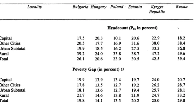
Almost all empirical work on poverty in Eastern Europe and the FSU has identified a strong correlation between household size and composition and poverty incidence. In Eastern Europe, the correlation is strongest with number of children. In each of the three countries analyzed here, households with three or more children have poverty incidence about double the national rate (Table 2). It does not matter much whether this is a nuclear household or an extended household with more than two adults. The exception is Hungary where the poverty rate in extended households with three or more children is more than triple the national rate. This is because in Hungary extended households often
arise as a result of poverty, which forces separate households to merge in order to benefit from economies of scale in housing and other expenditures.
The implication is that in Eastern Europe, poverty among children is higher than average and the presence of children needs to be considered as a strong candidate indicator for targeting. We will revisit this proposition in the following sections when reviewing the multivariate results. The finding of a strong correlation between poverty and the presence of children also constitutes a call to reform entitlement programs such as family allowances which provides fixed amounts of money to households with children. These allowances are probably not needed by the richer households, and they are clearly insufficient to prevent households with many children from falling into poverty. A possible solution is to introduce means-testing and to increase the amounts given to large
Table 2: Poverty and Family Composition
Bulgaria Hungary Poland Estonia Kyrgyz Russia Republic
Family Composition
Headcount (P0, in percent)
One Male Adult, No Children 33.1 24.2 15.6 32.5 40.0 52.5 One Female Adult, No Children 45.0 27.8 13.5 37.0 51.8 47.8 One Adult, One or More Children 23.4 32.1 28.2 43.5 39.7 45.0 Two Adults, No Children 27.4 17.9 12.2 28.2 40.1 37.4
Two Adults, One Child 15.2 20.1 16.1 30.5 42.4 37.0
Two Adults, Two Children 19.4 19.9 24.7 29.6 39.9 38.7 Two Adults, Three or More Children 61.3 38.1 43.3 28.5 49.1 64.2 Three or More Adults, No Children 22.7 13.9 16.6 24.4 37.0 30.2 Three or More Adults. One Child 20.1 17.7 20.2 27.8 35.6 35.8 ThreeorMoreAdults.TwoChildren 35.8 29.5 36.2 31.6 43.3 51.6 Three or More Adults, Three or More 55.9 71.1 46.2 57.6 43.6 60.4 Children
All 26.1 20.6 23.0 30.5 42.5 39.4
Poverty Gap (in percent) 11
One Male Adult, No Children 26.0 17.9 22.4 34.3 39.5 42.0 One Female Adult, No Children 28.9 18.6 17.3 27.5 47.4 44.2 One Adult, One or More Children 25.0 20.8 19.7 24.3 26.8 35.9 Two Adults, No Children 20.8 13.8 14.5 20.3 31.8 33.5
Two Adults, One Child 14.3 15.1 13.6 18.8 27.7 26.9
Two Adults, Two Children 18.1 13.1 12.8 17.4 26.7 27.0 Two Adults, Three or More Children 22.0 13.5 13.6 16.8 27.0 28.3 Three or More Adults, No Children 16.2 12.6 13.2 17.3 26.2 27.6 Three or More Adults, One Child 18.6 12.7 12.5 16.2 21.8 26.1 Three or More Adults, Two Children 19.3 12.8 12.8 16.6 23.0 25.0 Three or More Adults, Three or More 24.5 13.8 11.7 17.1 22.8 26.6 Children
All 19.8 14.1 13.3 20.2 25.0 29.8
Source: Household Expenditure and Income Date for Transition Economies Data Set (HEIDE). Notes:
1/ The poverty gap is the poor's average shortfall in expenditures from the poverty line, expressed as a percentage of the poverty line (this measure is also known as the expenditure gap ratio).
poor households. Grootaert (1995, 1997a) contains simulation exercises which demonstrate, in the cases of Poland and Hungary, that this can be achieved in a budget-neutral fashion, and that it has the potential of significantly reducing poverty among children. In part, the potential success from introducing means-testing results from the fact that the poverty gap is not higher among households with many children. This means that on a per capita basis, the resources needed to lift these households out of poverty is not greater than for other kinds of households. In fact, the uniformnity of the poverty gap
across different types of households, displayed in Table 2, is quite a remarkable feature of poverty in Eastern Europe.
Apart from large households, poverty incidence is also above average in households with one adult. The situation is especially bad in Bulgaria among women
living alone, where poverty incidence is 45%. Most of these are pensioners. In Poland, in
contrast, households consisting of one man or one woman have below average poverty
rates, reflecting that pensions in Poland are higher than elsewhere. In Hungary and
Poland, one-adult households with children have higher poverty rates than those without
children, and there is some evidence that such households are more likely to fall through
the cracks of the family allowance system and to not receive these benefits (Grootaert,
1995, 1997a). Poor one-adult households also experience deeper poverty than other poor
households: in all three countries, they have larger poverty gaps than any other type of households.
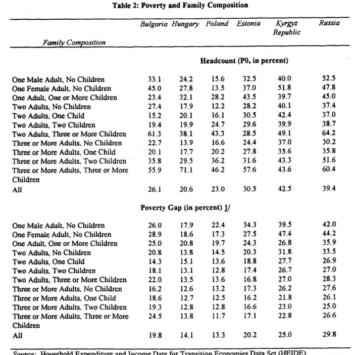
While Table 2 expresses the composition of the household in terms of the number
the adults is also correlated with poverty. Except in Poland, households consisting only of
elderly have the highest poverty incidence and poverty gap. We return to this later when
discussing the age-dimension of poverty.
Table 3: Poverty and Aggregate Family Composition
Bulgaria Hungary Poland Estonia Kyrgyz Russia Republic Family Composition Headcount (P0, in percent) No Children, No Elderly 18.3 13.0 13.3 23.8 37.6 31.9 Child(ren), No Elderly 25.0 23.9 28.1 32.8 43.1 40.5 No Children, Elder(ly), 39.0 26.1 18.1 39.4 43.8 43.8 Child(ren), Elder(ly) 28.0 22.2 32.7 35.2 42.9 51.5 All 26.1 20.6 23.0 30.5 42.5 39.4
Poverty Gap (in percent) V1
No Children, No Elderly 18.8 13.6 13.6 22.0 29.4 32.2 Child(ren), No Elderly 19.4 14.1 13.2 18.3 24.2 27.1 No Children, Elder(ly) 21.1 15.1 15.5 22.8 34.0 35.5
Child(ren), Elder(ly) 19.5 10.5 11.9 19.2 23.9 27.0
All 19.8 14.1 13.3 20.2 25.0 29.8
Source: Household Expenditure and Income Date for Transition Economies Data Set (HEIDE). Notes:
I/ The poverty gap is the poor's average shortfall in expenditures from the poverty line, expressed as a percentage of the poverty line (this measure is also known as the expenditure gap ratio).
Labor Force Participation
It is not surprising that labor force status is strongly correlated with poverty
outcomes in Eastern Europe. In all countries, wage earners and the self-employed have
the lowest poverty incidence and poverty gap (Table 4). Which of these two groups does
best depends on the stage of transition. In Hungary, with perhaps the best developed
private sector, and the earliest initiation of transition, the self-employed have the lowest
poverty incidence-slightly more than half the national rate. Elsewhere though,
wage-work still provides the better alternative.
Table 4 also shows though that being a pensioner sharply increases the odds of
being poor, except in Poland, and in all countries pensioners have above average poverty
gaps. The favorable situation of pensioners in Poland is due to the generosity of the Polish
pension system. Of all East European countries, Poland increased spending on pensions
the most: between 1988 and 1993, pension spending rose from 6.9 percent to 14.7 percent
of GDP (Perraudin and Pujol, 1994). One reason for this was the sudden swelling of the
ranks of pensioners by 1.5 million early retirees in the period 1989-1992. Furthermore, in
1992-93, the average pension in Poland was 64 percent of the average wage-the highest
ratio in Eastern Europe. Polish pensions were at that time also fully indexed (Milanovic,
1995). 10
I0 The pension systen in Poland is discussed in detail in World Bank (1993) and Peffaudin and Pujol (1994). For a
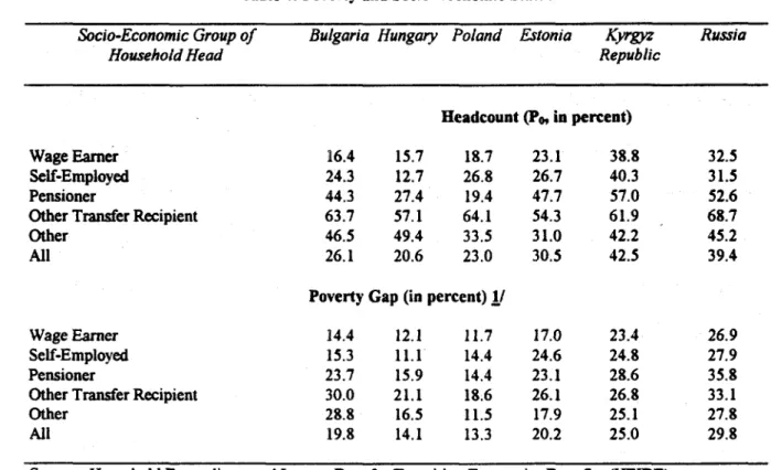
Table 4: Poverty and Socio-Economic Status
Socio-Economic Group of Bulgaria Hungary Poland Estonia Kyrgyz Russia
Household Head Republic
Headcount (Po, in percent)
Wage Earner 16.4 15.7 18.7 23.1 38.8 32.5
Self-Employed 24.3 12.7 26.8 26.7 40.3 31.5
Pensioner 44.3 27.4 19.4 47.7 57.0 52.6
Other Transfer Recipient 63.7 57.1 64.1 54.3 61.9 68.7
Other 46.5 49.4 33.5 31.0 42.2 45.2
All 26.1 20.6 23.0 30.5 42.5 39.4
Poverty Gap (in percent) 1/
WageEarner 14.4 12.1 11.7 17.0 23.4 26.9
Self-Employed 15.3 11.1 14.4 24.6 24.8 27.9
Pensioner 23.7 15.9 14.4 23.1 28.6 35.8
Other Transfer Recipient 30.0 21.1 18.6 26.1 26.8 33.1
Other 28.8 16.5 11.5 17.9 25.1 27.8
All 19.8 14.1 13.3 20.2 25.0 29.8
Source: Household Expenditure and Income Date for Transition Economies Data Set (HEIDE). Notes:
1/ he poverty gap is the poor's average shortfall in expenditures from the poverty line, expressed as a percentage of the poverty linc (this measure is also known as the expenditure gap ratio).
While the self-employed are a new socioeconomic category in countries in transition, representing people who have succeeded in adapting economically to transition,
there is also another socioeconomic category emerging of people who have fallen victim
to transition: those who have severed ties to the labor market, and who are unemployed
or irregularly employed, and for whom as a result transfer income (other than pensions)
has become the main source of income. This category of people has poverty rates that are around 60 percent, and they also have poverty gaps which are above average. However,
except for this category of households, Table 4 again confirms the remarkable evenness of
the poverty gap across society. We already pointed at the uniformity of the poverty gap
across demographic types of households (Table 2) and the same uniformity is seen across
socioeconomic categories.
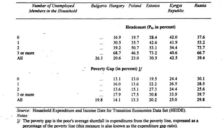
The specific effect of being unemployed is illustrated in Table 5 which shows the
poverty measures by the number of unemployed household members. In Hungary,
households without unemployed members have a poverty incidence of 16.9 percent. If
one household member is unemployed, the figure jumps to 30.5 percent, and it rises
further to 68.7 percent if three or more members are unemployed. In Poland, poverty
incidence is 19.7 percent in households without an unemployed member but 50.7 percent
in households with two unemployed members. Again though, the poverty gap is not
systematically related to the number of unemployed household members, indicating that
the social safety net does what it is supposed to do, namely preventing the emergence of
pockets of deep poverty. (Of course, this finding does not consider overall cost or
Table 5: Poverty and Unemployment
Number of Unemployed Bulgaria Hungary Poland Estonia Kyrgyz Russia
Members in the Household Republic
Headcount (P0, in percent) 0 ... 16.9 19.7 28.4 42.0 37.6 1 .. 30.5 35.7 42.6 41.9 53.2 2 ... 39.2 50.7 53.1 54.4 73.7 3 or more ... 68.7 46.5 73.2 40.6 66.7 All 26.1 20.6 23.0 30.5 42.5 39.4
Poverty Gap (in percent) V/
0 ... 13.1 13.0 19.5 24.4 30.1
1 ... 16.0 13.6 22.2 26.5 28.5
2 ... 13.6 15.1 27.3 24.4 25.6
3 or more ... 17.9 17.5 30.8 33.9 39.7
All 19.8 14.1 13.3 20.2 25.0 29.8
Source: Household Expenditure and Income Date for Transition Economies Data Set (HEIDE). Notes:
I/ The poverty gap is the poor's average shortfall in expenditures from the poverty line, expressed as a
percentage of the poverty line (this measure is also known as the expenditure gap ratio).
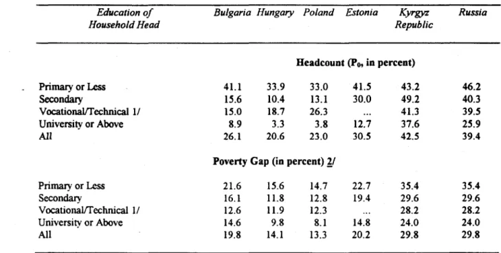
The role of education in this process is made clear in Table 6. There is a distinct
difference between the East European and the FSU countries. In Eastern Europe, the link
between lower poverty and higher education is extremely pronounced, but in the FSU this
link is much weaker, to being almost non-existent in Kyrgyz Republic. In Hungary, e.g.,
the poverty incidence among households where the head has primary education or less is
33.9 percent, while in households where the head has university education it is
Table 6: Poverty and Education
Education of Bulgaria Hungary Poland Estonia Kyrgyz Russia
Household Head Republic
Headcount (P0, in percent) Primary or Less 41.1 33.9 33.0 41.5 43.2 46.2 Secondary 15.6 10.4 13.1 30.0 49.2 40.3 Vocationa/Technical 1/ 15.0 18.7 26.3 ... 41.3 39.5 University or Above 8.9 3.3 3.8 12.7 37.6 25.9 All 26.1 20.6 23.0 30.5 42.5 39.4
Poverty Gap (in percent) 2/
Primary or Less 21.6 15.6 14.7 22.7 35.4 35.4
Secondary 16.1 11.8 12.8 19.4 29.6 29.6
VocationalTechnical 1/ 12.6 11.9 12.3 ... 28.2 28.2
Universitv or Above 14.6 9.8 8.1 14.8 24.0 24.0
All 19.8 14.1 13.3 20.2 29.8 29.8
Source: Household Expenditure and Income Date for Transition Economies Data Set (HEIDE). NVotes:
I/ For Estonia, secondary education and vocational-technical education are combined and shown in the category labeled "Secondary." Definitional problems in the Estonian dataset precluded a separation of these two kinds of education.
2J/ The poverty gap is the poor's average shortfall in expenditures from the poverty line, expressed as a percentage of the poverty line (this measure is also known as the expenditure gap ratio).
This difference in the impact of education is clearly related to the stage of transition. The further advanced transition is, the more a private sector emerges which needs well-educated workers, with general education backgrounds which makes them flexible and adaptable to the newly emerging skill requirements. Pre-transition vocational and technical education, often geared towards traditional industrial occupations, is no longer in demand. Similarly, low-skill jobs, of the type held by workers with primary education or less, have disappeared in great numbers. The more advanced transition countries such as Hungary and Poland have already experienced skill-shortages in fields like engineering, computer science and the like, and this will further push up wages received by workers with university education, and increase the wage-gap across skill-levels. This is one of the main reasons why the distribution of wages has increased in many transition economies (Milanovic, 1995, 1997).
Education is also the only dimension where the wage gap is not uniform across
categories in Eastern Europe. Workers with primary or less education have not only poverty rates well above average, but the poverty gap is also significantly higher than for other groups. Households where the head has a university education have the lowest poverty gap of any category, along any dimension, displayed in the poverty profile. It may be surprising that the poverty gap varies so much with education level, while it varies very little with the number of unemployed in the household. In part, the reason is that education is not used as a targeting variable for any transfer program (although our results
unemployment, many people with low education still hold full-time jobs (let us not forget
that they are a very large category: in Poland and Hungary, about two-thirds of
households have heads with primary or vocational/technical education). Their wages are
low, and as our results indicate, often insufficient to keep them above the poverty line. Still, as full-time workers, they do not qualify for any transfers (other than general
entitlements) to supplement their income. There is no immediate solution to this situation.
In the medium to long term, retraining and a general upgrading of schooling curricula will
reduce the number of people with low education. Also, people with low education are
older than average, and many of them will become absorbed in the pension system in the
near term. Whether this will alleviate their poverty, depends partly upon policies
pertaining to minimum pensions.
Gender and Age
- We already noted the correlation between household composition and poverty
outcomes, especially the association between the presence of three or more children and
high poverty incidence. Since demographic household characteristics are easily observable
and potentially useful targeting variables, it is worthwhile to look in more detail at the age
and gender dimensions of poverty in Eastern Europe.
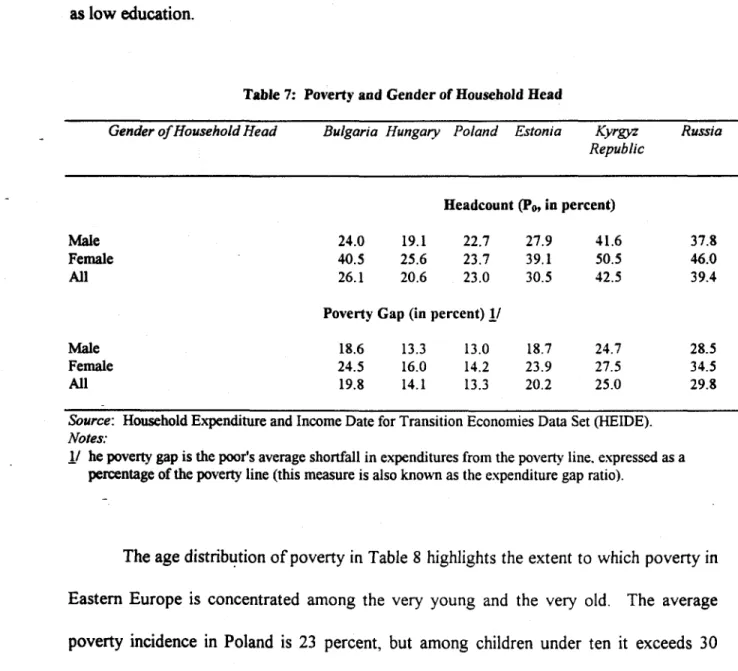
Table 7 shows that female-headed households have systematically higher poverty
incidence and poverty gaps than male-headed households. The difference is slight in
Poland, but more pronounced in Hungary and Bulgaria. The multivariate analysis in the
characteristics of female-headed households that are strongly correlated with poverty such
as low education.
Table 7: Poverty and Gender of Household Head
Gender ofHousehold Head Bulgaria Hungary Poland Estonia Kyrgyz Russia Republic
Headcount (P0, in percent)
Male 24.0 19.1 22.7 27.9 41.6 37.8
Female 40.5 25.6 23.7 39.1 50.5 46.0
All 26.1 20.6 23.0 30.5 42.5 39.4
Poverty Gap (in percent) 11
Male 18.6 13.3 13.0 18.7 24.7 28.5
Female 24.5 16.0 14.2 23.9 27.5 34.5
All 19.8 14.1 13.3 20.2 25.0 29.8
Source: Household Expenditure and Income Date for Transition Economies Data Set (HEIDE).
Notes:
I/ he poverty gap is the poor's average shortfall in expenditures from the povertv line, expressed as a percentage of the poverty line (this measure is also known as the expenditure gap ratio).
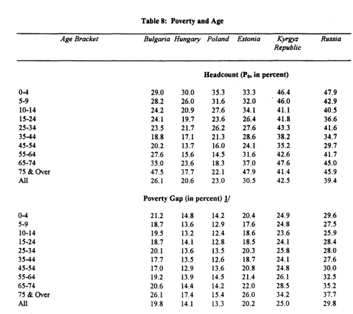
The age distribution of poverty in Table 8 highlights the extent to which poverty in Eastern Europe is concentrated among the very young and the very old. The average poverty incidence in Poland is 23 percent, but among children under ten it exceeds 30 percent. The numbers for Hungary show a similar pattern. In Bulgaria, the relative concentration of poverty among children is actually least. This is not a contradiction with the earlier finding that in Bulgaria poverty rates among households with three or more
Table 8: Poverty and Age
Age Bracket Bulgaria Hungary Poland Estonia Kyrgyz Russia Republic
Headcount (Po, in percent)
0-4 29.0 30.0 35.3 33.3 46.4 47.9 5-9 28.2 26.0 31.6 32.0 46.0 42.9 10-14 24.2 20.9 27.6 34.1 41.1 40.5 15-24 24.1 19.7 23.6 26.4 41.8 36.6 25-34 23.5 21.7 26.2 27.6 43.3 41.6 35-44 18.8 17.1 21.3 28.6 38.2 34.7 45-54 20.2 13.7 16.0 24.1 35.2 29.7 55-64 27.6 15.6 14.5 31.6 42.6 41.7 65-74 35.0 23.6 18.3 37.0 47.6 45.0 75 & Over 47.5 37.7 22.1 47.9 41.4 45.9 All 26.1 20.6 23.0 30.5 42.5 39.4
Poverty Gap (in percent) j/
0-4 21.2 14.8 14.2 20.4 24.9 29.6 5-9 18.7 13.6 12.9 17.6 24.8 27.5 10-14 19.5 13.2 12.4 18.6 23.6 25.9 15-24 18.7 14.1 12.8 18.5 24.1 28.4 25-34 20.1 13.6 13.5 20.3 25.8 28.0 35-44 17.7 13.5 12.6 18.7 24.1 27.6 45-54 17.0 12.9 13.6 20.8 24.8 30.0 55-64 19.2 13.9 14.5 21.4 26.1 32.5 65-74 20.6 14.4 14.2 22.0 28.5 35.2 75 & Over 26.1 17.4 15.4 26.0 34.2 37.7 All 19.8 14.1 13.3 20.2 25.0 29.8
Source: Household Expenditure and Income Date for Transition Economies Data Set (HEIDE). Notes:
1/ The poverty gap is the poor's average shortfall in expenditures from the poverty line, expressed as a percentage of the poverty line (this measure is also known as the expenditure gap ratio).
Poverty incidence in Eastern Europe decreases with age, and reaches a minimum at
ages 35-44 in Bulgaria, ages 45-54 in Hungary, and ages 55-64 in Poland. After those
ages, the increase in poverty incidence is quite rapid and severe, except in Poland (as we
noted earlier, this is due to the generous pension system in Poland). In Bulgaria and
Hungary, poverty rates among people over 75 are close to twice the national average.
The vast majority of people in that age group are women, and their poverty rates are
higher than for the men in that group. Actually, the gender-breakdown of Table 8 (not
shown here) reveals that poverty rates among the elderly are higher for women in general
than for men. At lower ages though, the gender gap is not very pronounced, and for some
ages poverty is lower among women than men.
Gender is thus a relevant poverty dimension in Eastern Europe primarily for the elderly, especially at very high ages, and for female-headed households. For many women, the labor market changes of transition have had major implications. Prior to transition,
women were expected to work full-time but the state provided day care for their children.
Transition has led to a drop in female labor force participation (not all of it voluntarily) but it has also led to a reduced supply of affordable day care centers (World Bank, 1996e)." Both factors may well affect female-headed households disproportionately.
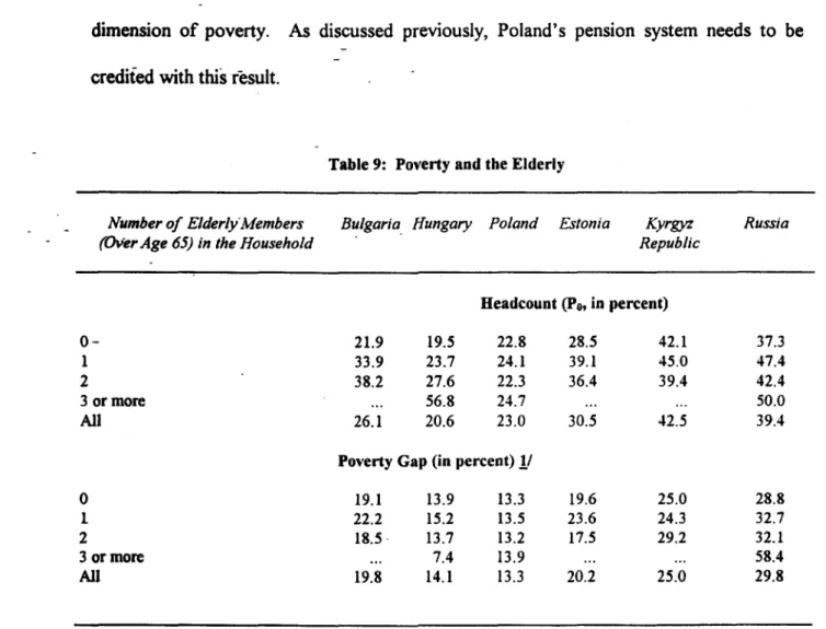
Nevertheless, the poverty figures suggest that in general the age-effect outweighs the gender-effect. This is clear also from Table 9 which classifies households by the number of elderly people (over 65) in the household. In Bulgaria and Hungary, households without elderly members have below average poverty rates and those with elderly members have above average poverty incidence. The latter increases with the number of elderly. Poland is again the exception, where age proves to be an irrelevant dimension of poverty. As discussed previously, Poland's pension system needs to be credited with this result.
Table 9: Poverty and the Elderly
Number of ElderlyMembers Bulgaria Hungary Poland Estonia Kyrgyz Russia
(Over Age 65) in the Household Republic
Headcount (Po, in percent)
0- 21.9 19.5 22.8 28.5 42.1 37.3
1 33.9 23.7 24.1 39.1 45.0 47.4
2 38.2 27.6 22.3 36.4 39.4 42.4
3 or more ... 56.8 24.7 ... ... 50.0
All 26.1 20.6 23.0 30.5 42.5 39.4
Poverty Gap (in percent) j/
0 19.1 13.9 13.3 19.6 25.0 28.8
1 22.2 15.2 13.5 23.6 24.3 32.7
2 18.5 13.7 13.2 17.5 29.2 32.1
3 or more ... 7.4 13.9 ... ... 58.4
All 19.8 14.1 13.3 20.2 25.0 29.8
Source: Household Expenditure and Income Date for Transition Economies Data Set (HEIDE). Notes:
V The poverty gap is the poor's average shortfall in expenditures from the poverty line, expressed as a percentage of the poverty line (this measure is also known as the expenditure gap ratio).
The poverty gap shows little variation by age, although it is above average among people aged over 65. It does not however increase systematically with the number of elderly in a household. In fact, in Hungary, it is the reverse-the poverty gap falls significantly in households with two or three elderly members. Many such households are poor, but they are not very far below the poverty line.
a& Former Soviet Union\
Poverty is generally considered to have sharply increased in countries undergoing transition, partly because incomes are perceived to have become extremely unequally distributed, and mostly as a result of drastic declines in GDP. Indeed, a static comparison of the poverty rates for the FSU suggests that poverty is a serious problem in Russia and Estonia, and a nearly overwhelming one in the Kyrgyz Republic.
After five years of economic contraction, the poor in the FSU appear to be primarily the working poor, and especially the working poor with children. The working poor are testimony to the adjustment in wages, rather than in open unemployment, which has occurred. The myth of the pensioner--he idea that pensioners are especially vulnerable to poverty-is belied by several studies, including this one (World Bank, various poverty assessments in transition economies), although it is true that the extremely elderly (aged 75 and over) are more vulnerable to poverty. This sketch of the poverty