Efficient Interference-Aware TDMA Link Scheduling
for Static Wireless Networks
Weizhao Wang
†Yu Wang
∗Xiang-Yang Li
†Wen-Zhan Song
‡Ophir Frieder
††
Department of Computer Science, Illinois Institute of Technology, Chicago, IL 60616, USA ∗
Department of Computer Science, University of North Carolina at Charlotte, Charlotte, NC 28223, USA ‡
School of Engineering and Computer Science, Washington State University, Vancouver, WA 98686, USA
ABSTRACT
We study efficient link scheduling for a multihop wireless network to maximize its throughput. Efficient link scheduling can greatly reduce the interference effect of close-by transmissions. Unlike the previous studies that often assume a unit disk graph model, we assume that different terminals could have different transmission ranges and different interference ranges. In our model, it is also possible that a communication link may not exist due to barriers or is not used by a predetermined routing protocol, while the trans-mission of a node always result interference to all non-intended re-ceivers within its interference range. Using a mathematical formu-lation, we develop synchronized TDMA link schedulings that opti-mize the networking throughput. Specifically, by assuming known link capacities and link traffic loads, we study link scheduling un-der the RTS/CTS interference model and the protocol interference model with fixed transmission power. For both models, we present both efficient centralized and distributed algorithms that use time slots within a constant factor of the optimum. We also present effi-cient distributed algorithms whose performances are still compara-ble with optimum, but with much less communications. Our theo-retical results are corroborated by extensive simulation studies.
Categories and Subject Descriptors
C.2.1 [Network Architecture and Design]: Wireless communi-cation; G.2.2 [Graph Theory]: Network problems, Graph algo-rithms.
General Terms
Algorithms, Design, Theory.
Keywords
Link scheduling, Interference, Graph Coloring, Distributed Algo-rithm, Wireless Networks.
∗
This work of Yu Wang was supported, in part, by funds provided by Oak Ridge Associated Universities.
†
The work of Xiang-Yang Li was partially supported by NSF CCR-0311174.
Permission to make digital or hard copies of all or part of this work for personal or classroom use is granted without fee provided that copies are not made or distributed for profit or commercial advantage and that copies bear this notice and the full citation on the first page. To copy otherwise, to republish, to post on servers or to redistribute to lists, requires prior specific permission and/or a fee.
MobiCom’06, September 23–26, 2006, Los Angeles, California, USA.
Copyright 2006 ACM 1-59593-286-0/06/0009 ...$5.00.
1.
INTRODUCTION
Wireless multi-hop radio networks such as ad hoc, mesh, or sen-sor networks are formed of autonomous nodes communicating via radio. Wireless networks draw lots of attentions in recent years due to their potential applications in various areas. For example, wireless mesh networks are being used as the last mile for extend-ing the Internet connectivity for mobile nodes. These networks be-have almost like wired networks since they be-have infrequent topol-ogy changes, limited node failures, etc.. For wireless mesh net-works or sensor netnet-works, the aggregate traffic load of each routing node changes infrequently also. A unique characteristic of wire-less networks is that the radio sent out by a wirewire-less terminal will be received by all the terminals within its transmission range, and also possibly causes signal interference to some terminals that are not intended receivers. In other words, the communication chan-nels are shared by the wireless terminals. Thus, one of the major problems facing wireless networks is the reduction of capacity due to interference caused by simultaneous transmissions. Using mul-tiple channels and mulmul-tiple radios can alleviate but not eliminate the interference. To achieve robust and collision free communica-tion, there are two alternatives. One is to utilize a random access MAC layer scheme. The other is to carefully construct a transmis-sion schedule. One variant, link scheduling in the context of time division multiplexing (TDM) is the subject of this paper.
In this paper, we assume that the time is slotted and synchro-nized. A link scheduling is to assign each link a set of time slots
⊂[1, T]on which it will transmit, whereT is the scheduling pe-riod. A link scheduling is interference-aware (or called valid) if a scheduled transmission on a linkx→ywill not result in a collision at either nodexor nodey(or any other node). In this context, two types of collisions must be avoided, namely, primary interference and secondary interference. Link scheduling has received a great attention from both networking and theory fields [1, 16–21, 23, 26] in the past few years due to its application for assigning time slots in TDMA MAC protocols that eliminate collision, guarantee fair-ness. Many scheduling problems in wireless networks have been shown to be NP-complete, including TDMA broadcast schedul-ing [7], link schedulschedul-ing [2, 8]. For some of these problems, even polynomial-time algorithms with constant approximation ratios ap-pear unlikely for general graphs.
Previous studies on link scheduling either assume a very gen-eral graph model or assume a very specific graph model such as unit disk graph (UDG). It is widely accepted in the wireless net-working community that neither a general graph model nor UDG model accurately captures unique properties of wireless networks. A general graph model could not capture a certain geometry prop-erty of wireless networks, e.g., two nodes must be within certain distance to be able to communicate directly (or one node’s
trans-mission could interfere the other node’s reception). A unit disk graph model is idealistic since in practice two nearby nodes may still be unable to communicate due to various reasons such as bar-rier and path fading. In this paper, we give efficient centralized and distributed algorithms to obtain a valid link scheduling with theo-retically proven performances for a more realistic wireless network model. The main contributions of this paper are as follows.
• More Realistic Model: We address the link scheduling in a
more realistic networking model: (1) each node has its own transmission power and thus its own transmission range; (2) that the receiver must be within the transmission range of the sender is only a necessary (but not sufficient) condition for two nodes to communicate directly, i.e., two nearby nodes may still be unable to communicate directly; (3) if a nodev
is within certain distance of a senderu, then the transmission byuwill interfere the reception of nodev. In summary, the communication graph could be an arbitrary geometry graph. Notice that similar realistic models using weighted and un-weighted flows, modeling interference range to be different from transmission range, etc. have all been proposed and modeled in earlier work, e.g. in [15, 18, 21], and heuristic algorithms have been given for each or all of these. Our contributions here are that we provide theoretical bounds for link-scheduling algorithms in these cases.
• Both Weighted and Unweighted Flow: In several wireless
networks (e.g., mesh, sensor networks), we can estimate the traffic demand by each wireless node. Thus, based on a given routing algorithm, we can predict the average traffic load`(e) on each linkeof the network. We then design link scheduling algorithms to meet this traffic demand if possible. We model this by assuming that each linkehas an integral weightw(e) specifying the number of slots it needed in a period to sup-port its traffic load. Herew(e) =dT ·`(e)
c(e)e, wherec(e)is
the capacity of linkeif there is no interference, andT is a given period for a schedule. In certain networks, it is diffi-cult, if not impossible, to estimate the load of every link. We then assume that each node needs at least one time slot for transmission and our objective is to design a scheduling that minimizesT.
• Theoretical Performance Guarantee for Efficient
Central-ized/Distributed Algorithms: We consider two kinds of
in-terference models: RTS/CTS model and protocol interfer-ence model with fixed transmission power. For both models, we present both centralized and distributed link scheduling algorithms that use time slots at most a constant factor of the optimum. All algorithms involve a novel study of interfer-ence properties in wireless networks. For the protocol in-terference model, we require that the inin-terference range of a node is larger than its transmission range, which is always true in practice (the interference range of a node is about twice of its transmission range). One of our distributed al-gorithms has not only small communication complexity, but also good performance guarantee that is only logarithmic of the ratio between the maximum and minimum interference range. Although some of our algorithms are similar to some algorithms proposed before, to the best of our knowledge, we are the first one to prove asymptotical optimal bounds for the performance. We also present both necessary and sufficient conditions for schedulable flows under interference.
• Layer Independence: To preserve the independence between
layers, we assume that there is already an existing routing al-gorithm that will select a path for every pair of source and destination nodes. The performance guarantee of methods
presented here is independent of the routing algorithm when the routing is given. The results presented here can also be extended to the scenario when we want to maximize the throughput by optimizing the routing and TDMA link schedul-ing together.
The rest of the paper is organized as follows. In Section 2, we discuss the network models and interference models and formally define the problem studied in this paper. We present our central-ized algorithms for link scheduling in Section 3. We also analyze the theoretical guaranteed performances of our algorithms. Our distributed algorithms are presented in Section 4. In Section 5, we study how to assign time slots to links when each link has a re-quirement of the least number of time slots needed. Our simulation studies are reported in Section 6. In Section 7, we briefly review the related works in the literature. We conclude our paper in Section 8.
2.
SYSTEM MODEL AND ASSUMPTIONS
Interference issues have been studied extensively recently be-cause it is widely believed that reducing the interference can in-crease the overall performance of a wireless network. There are dif-ferent approaches to reduce the interference, including the schedul-ing on the MAC layer, route selection on the routschedul-ing layer and power control on the physical layer. In this section, we first discuss in detail the interference models we will use and formally define the problem that we will study in this paper.
2.1
Network and Interference Models
NETWORK MODEL: In this paper, we assume that there is a set
V of communication terminals deployed in a plane. Each wireless terminal is only equipped with single radio interface. The com-plete communication graph is a directed graphG= (V, E), where
V ={v1, . . . , vn}is the set of terminals andEis the set of pos-sible directed communication links. Every terminalvihas a trans-mission rangeti such that the necessary condition for a terminal
vjto receive correctly the signal fromviiskvi−vjk ≤ti, where kvi−vjk(sometimes we denote it asdi,j for simplicity) is the Euclidean distance betweenviandvj. Notice thatkvi−vjk ≤ti is not the sufficient condition for (vi, vj) ∈ E. Some links do not belong toGbecause of either the physical barriers or the se-lection of routing protocols. This is the major distinction of our model with the majority previous studies on link scheduling. To the best of our knowledge, only [21] used the similar model as ours. We always useli,j to denote (vi, vj) hereafter. Each ter-minalvialso has an interference rangerisuch thatvjis interfered by the signal fromviifkvi−vjk ≤riandvjis not the intended receiver. The interference rangeriis not necessarily same as the transmission rangeti. Typically,ri> ti. We call the ratio between them as the Interference-Transmission Ratio for nodevi, denoted asγi = rti
i. In practice,2≤γi ≤ 4. For all wireless nodes, let
γ= maxvi∈V ri ti.
INTERFERENCEMODELS: To schedule two links at the same time slot, we must ensure that the schedule will avoid the interference. Two different types of interference have been studied in the lit-erature, namely, primary interference and secondary interference. Primary interference occurs when a node transmits and receives packets at the same time. Secondary interference occurs when a node receives two or more separate transmissions. Here all trans-missions could be intended for this node, or only one transmission is intended for this node (thus, all other transmissions are interfer-ence to this node). In addition to these interferinterfer-ences, there could have some other constraints on the scheduling, e.g., the radio net-works that deploy the IEEE802.11protocol with request-to-send
and clear-to-send (RTS/CTS) mechanism will pose some additional constraints. Several different interference models have been used to model the interferences in wireless networks. We briefly review them in the following.
Protocol Interferences Model (PrIM): It was first proposed
in [13]. In this model, a transmission by a nodeviis successfully received by a nodevjiff the intended destinationvjis sufficiently apart from the source of any other simultaneous transmission, i.e.,
kvk−vjk ≥(1 +η)kvi−vjkfor any nodevk 6=vi. Here con-stantη >0models situations where a guard zone is specified by the protocol to prevent a neighboring node from transmitting on the same channel at the same time. This model implicitly assumed that each nodevkwill adopt the power control mechanism when it transmits signals. Simulation analysis [12] as well as the analyt-ical results [3] indicate that the protocol interference model does not necessarily provide a comprehensive view of reality due to the aggregate effect of interference in wireless networks. However, it does provide some good estimations of interference and most im-portantly it enables a theoretical performance analysis of a num-ber of protocols designed in the literature. Link scheduling using PrIM interference model and network model similar to ours has been studied in [21].
Fixed Power Protocol Interferences Model (fPrIM): We adopt
the following interference model throughout this paper. We assume that a node will not dynamically change its power based on the intended receiver in a packet-level. Note that this assumption does not preclude the power control that can further reduce the power consumption. We only assume that there is no power adaptation at the packet level and the power is not adjustable for a certain period of time, which is close to the real situation. However, we do assume that each nodevihas its own fixed transmission power and thus a fixed transmission rangeti. We also assume that each nodevkhas an interference rangerksuch that any nodevjwill be interfered by the signal fromvkifkvk−vjk ≤rkand nodevkis sending signal to some node other thanvj. In other words, the transmission from
vitovjis viewed successful ifkvk−vjk> rkfor every nodevk transmitting in the same time slot using the same channel.
RTS/CTS Model: This model was also studied previously, e.g.,
[1]. For every pair of transmitter and receiver, all nodes that are within the interference range of either the transmitter or the receiver cannot transmit. Figure 1(a) shows the case that communication fromB to Aand Cto D cannot take place simultaneously due to RTS. Figure 1(b) shows the case that communication fromA
toB andD toC cannot take place simultaneously due to CTS. Although RTS/CTS is not the interference itself, for convenience of our notation, we will treat the communication restriction due to RTS/CTS as RTS/CTS interference model. Thus, for every pair of
D B
A C A B C D
(a) Due to RTS (b) Due to CTS
Figure 1: Communication Restriction by RTS/CTS.
simultaneous communication links, sayvivj andvpvq, it should satisfy that (1) they are distinct four nodes, i.e.,vi 6=vj 6=vp 6=
vq; (2)viandvjare not in the interference ranges ofvpandvq, and vice versa. The interference region, denoted byIi,j, of a linkli,j is the union of the interference region of nodesviandvj. When a directed linkvivj(orvjvi) is active, all simultaneous transmitting linksvpvqcannot have an end-point inside the areaIi,j. Notice, it
is possible that neithervpnorvq is inIi,j butlp,qstill interferes withli,jsinceviorvjmay be insideIp,q.
Physical Interference Model (PhIM): In this model, the
signal-to-interference-and-noise ratio (SINR) is used to describe the ag-gregate interference in the network. The transmission from node
viis successfully received at nodevjif and only if the SINR is at least the minimum SINR threshold required by nodevj.
In this paper, we mainly focus on link scheduling for the fPrIM model and the RTS/CTS model. Notice that these two models are different. For example, in Figure 1(a), linksBAandCDcan be assigned the same channel in the protocol interference model, but not in the RTS/CTS model. Similar statement holds for linksAB
andDCin Figure 1(b).
2.2
Problem Formulation
Assume that the communication links in the wireless network are predetermined, either by some existing routing protocol as AODV, DSR or can be predicted from the existing routes. Given a commu-nication graphG = (V, E), we use the conflict graph (e.g., [15])
FGto represent the interference inG. Each vertex (denoted byli,j) ofFGcorresponds to a directed link(vi, vj)in the communication graphG. There is an edge between vertexli,jand vertexlp,qinFG if and only ifli,jconflicts withlp,qdue to interference. Recall that whether two links conflict depends on the interference model used underneath, e.g., protocol interference model or RTS/CTS model. Thus, for a given communication graphG, the interference graph
FGmay be different. To avoid the confusion, we useFGPto denote the interference graph under the protocol interference model and
FD2
G to denote interference graph under RTS/CTS model. Our objective is to give each linkl∈Ga transmission schedule
S(l), which is the list of time slots it could send packets such that the schedule is interference-free and the overall throughout of the network is maximized. LetXe,t∈ {0,1}be the indicator variable which is1iffewill transmit at timet. We will focus on periodic schedules in this paper. A schedule is periodic with periodTif, for every linkeand time slott,Xe,t=Xe,t+i·Tfor any integeri. For a linke, letI(e)denote the set of linkse0
that will cause interfer-ence ifeande0
are scheduled at the same time slot. A schedule
S is interference-free ifXe,t+Xe0,t ≤ 1for anye0 ∈ I(e). In the graph theory terminology, the interference free link scheduling problem is essentially the vertex coloring ofFG.
When the traffic load of links are unknown, the objective of link scheduling is to find a scheduling with the minimum period. If we schedule all links within a periodχsuch that no two links in same time slot interfere with each other, then at least one packet can be delivered over each communication link in every χtime slots. Thus,1/χis often used to estimate the throughput of the network based on this schedule. The second case is that the average traffic load`(e)of each link is known in advance. We model this by assuming that each communication linke(vertex in the conflict graph) has a weightw(e)specifying the minimum number of time slots it required in each period. Herew(e) = dT · `(e)
c(e)e, where
c(e)is the capacity of linkeandT is a given period for a schedule. Our main focus in this paper is how to schedule the communication links in an interference-free manner such that the throughput of the network is maximized, i.e., with the smallestT.
There are a number of distinctions of the model used here with the models used in previous study: (1) We assume that each wire-less node has an interference range, which may be different from its transmission range; (2) We do not require the same transmission range (also same interference range) for every wireless node; (3) We do not require the communication graph to be complete, i.e., some communication links may not exist due to barriers or may be
not used by routing selection.
Notice that for simplicity we assume that there is only a single-channel in the network. All our results can be easily extended to the case when multiple channels are available as in [1]. If nodes has a pre-assigned channels for each link, then the link scheduling with multiple channels is just the simple union of a set of schedul-ings, where each scheduling is for all links using the same channel. However, we agree that the static assignment of correct channels to appropriate links is a bigger factor in determining the performance. If links can dynamically switch channels, then our greedy algo-rithms will find the channel with the smallest available time slot for each link to be scheduled and the same performances hold.
3.
CENTRALIZED SCHEDULING
In this section, we will propose centralized algorithms for link scheduling under different interference models. The performances of centralized algorithms will then be used as a certain benchmark to evaluate the performances of our distributed algorithms.
3.1
Scheduling under RTS/CTS Model
A number of centralized algorithms for link scheduling have been proposed in the literature, e.g., [1, 21]. A common approach is to assign each link the best possible channels (smallest time slots here) by greedy. The difference between them is the processing or-der of links: [21] processes links with smaller lengths first while [1] processes links in an arbitrary order (since it uses UDG graph mod-els for both communication and interference). Our centralized al-gorithm is will process links in a special order as in [14]. The basic idea is to first sort links as follows: every time we pick a link, sayl, from the remaining graph that has the smallest number of interfered links in the remaining graph and then removelfrom this graph; re-peat this till the graph becomes empty. We then assign time slots to links in the reverse order of picked links using the smallest time slot available (not used by interfering links). In summary, a linkewith largerI(e)will be more likely processed earlier by our algorithm.
Algorithm 1 Centralized Scheduling under RTS/CTS Model
Input: A communication graphG= (V, E)ofmlinks.
Output: An interference-free link scheduling.
1: Construct the conflict graphFD2
G and let graphG0=FGD2. 2: whileG0is not empty do
3: Find the vertex with the smallest total degree inG0
and re-move this vertex fromG0
and all its incident edges. Letlk denote the(m−k+ 1)th vertex removed, and the degree of
lkin graphG0just before it is removed be itsδ-degree. 4: Process links froml1tolmand assign to eachlkthe smallest
time slot not yet assigned to any of its neighbors inFD2
G .
We first present some necessary definitions and properties needed to prove the performance of our algorithms. Given a communi-cation linkli,j, we define the interference radius of linkli,j as
ri,j = max{ri, rj}. Ifri > rj orri = rj and ID of nodevi is larger than the ID of nodevj, thenviis called the head (de-noted ashi,j) of link(vi, vj)and vj is the tail (denoted asti,j) of this link. Notice that here, the head of a link is not necessarily the sender of the directed communication link. Given a nodevk, we useR(vk, x)to denote the disk centered atvkand with radius
x·rk. A nodevkinterferes a nodeviif nodeviis inside the inter-ference region (i.e., diskR(vk,1)) of nodevk. We say a linklp,q interferes a nodevk if eithervporvq interferesvk. For a given nodevk, we useN≥(vk, α)to denote the set of nodes satisfying that (1) each of their interference radius is at leastrk; (2) each of
them interferes some nodes inR(vk, α). Notice that a node from
N≥(v
k, α)could be arbitrarily far away from nodevk. Similarly, for a link li,j, letR(li,j, x) denote the union of two disks cen-tered atviandvjrespectively with radiusx·riandx·rj respec-tively. LetN≥(l
i,j, α)denote the union of node setsN≥(vi, α) andN≥(v
j, α). The following theorem estimates the local chro-matic number based on node degree.
THEOREM 1. For a given node vk and any node set Vk ⊆
N≥(v
k, α)with constantα, there exists a subsetVk0 of Vk with
cardinality|Vk|/Cαsuch that each node interferes with each other,
whereCα≤(6α+ 1)2+ 11.
PROOF. We consider a partition ofVk: the nodes in and outside regionR(vk,3α), denoted byVk1andVk2respectively.
First, we consider the node setV1
k. Using a simple area argu-ment, there are at most π((3α+
1 2)rk)2 π(1 2rk)2 = (6α+ 1) 2 disks with radiusrk
2 can be placed inside the diskR(vk,3α). Thus, there
ex-ists a node set inV1
k with size at least|Vk1|/(6α+ 1)2 such that each node in the set interferes with each other.
k
v
v v va b k 3ark(a) Divide the space into11cones (b) Two nodes interfere in same cone
Figure 2: Illustration of the partition of the region.
Second, we consider the node setV2
k. We divide the whole space into11equal cones using11rays fromvkas shown Figure 2(a). If
vaandvbare in the same cone, then∠vavkvb<33◦. Letda,b= kva−vbk. Sinceva ∈N≥(vk, α),vainterfere with some nodes inR(vk, α),da,k≤ra+α·rk. Similarly,db,k≤rb+α·rk. Thus, max{da,k, db,k} ≤max{ra, rb}+α·rk. On the other hand, since bothvaandvbare outsideR(vk,3α),min{da,k, db,k} ≥3α·rk. As shown in Figure 2 (b), forvaandvb,
d2a,b < d2a,k+d2b,k−2 cos(33◦)·da,k·db,k = max{da,k, db,k}2+ min{da,k, db,k}2−
5
3max{da,k, db,k} ·min{da,k, db,k}
≤ max{da,k, db,k} max{da,k, db,k} −2 3min{da,k, db,k} ≤ (max{ra, rb}+α·rk)·[max{ra, rb}+α·rk−2α·rk] ≤ max{ra, rb}2−α2·rk2<max{ra, rb}2.
The transition between the second and third inequalities is because max{da,k, db,k} ≤max{ra, rb}+α·rkandmin{da,k, db,k} ≥ 3α·rk. Thus,vainterferes withvb. Therefore, each pair of nodes in the same cone interfere with each other. This proves that there exists a node set inV2
k with size at least|Vk2|/11such that the nodes in the set interfere with each other.
Consequently, there exists a node set with size at least max{|Vk1|/(6α+ 1)2,|Vk2|/11} ≥ |V1 k|+|Vk2| (6α+ 1)2+ 11 = |Vk| Cα such that all nodes in the set interfere with each other. Here,Cα≤ (6α+ 1)2 + 11, and we call it the α
-hop interference number. Notice that(6α+ 1)2+ 11
is an upper bound onCαand it can be improved by using a more tight analysis.
Table 1: Summary of Main Notations
Term Definition
vi a wireless node fromV ={v1, v2,· · ·, vn}
li,jor(vi, vj) edge/link betweenviandvj
tiandri transmission range and interference range ofvi
γiandγ γi=ri/ti,γis the maximum ratio for allvi
Ii,j,hi,j,ti,j interference region/head/tail of linkli,j
ri,j interference radius ofli,j,max{ri, rj}
Xe,t indicator variable whetheretransmits at timet
FD2
G interference graph under RTS/CTS model
FP
G interference graph under fPrIM model
δ(FX
G) maximumδ-degree in the interference graph ∆(FX
G) maximum degree in the interference graph
R(vk, x) the disk centered atvkand with radiusx·rk
R(li,j, x) the union of two disks centered at vi and vj re-spectively with radiusx·riandx·rj
N≥(v
k, α) the set of nodes who interferes some nodes in
R(vk, α)and has interference radius at leastrk
N≥(l
i,j, α) the union of node setsN≥(vi, α)andN≥(vj, α)
I≥(e)
the set of links with larger radius thaneand inter-fering witheunder RTS/CTS model
din/outi,j (G) incoming/outgoing degree of vertexli,jinG ∆in/out(G)
maximum incoming/outgoing degree ofG d≥i,j(FGD2) number of adjacent vertices that precedeli,j
φ(FD2
G ) maxli,jd
≥
i,j(FGD2)
Hi all links that containvias the head
Mi,Mi+,Mi− all links that∈/Hiand interfere withHi; all links inMithat precede every link inHi;Mi−Mi+
ψ ratio between max and min interference ranges
N≥(v
k, α, β) the set of nodes who interferes some nodes in
R(vk, α)and has interference radius at leastrβk
N≥(l
i,j, α, β) the union ofN≥(vi, α, β)andN≥(vj, α, β) ∆(α, β) maxli,j|N
≥(l
i,j, α, β)|
χ(FX
G) optimal number of colors for graphFGX
Mi.jin/out all incomging/outgoing links fromli,j
w(e),`(e),c(e) weight, traffic load and capacity of linke
Notice that Theorem 1 works for the interference on nodes only. For a linke=li,j, letI≥(e)be the linkse0interfering witheunder RTS/CTS model and whose radius is not smaller thane. Following theorem shows a counterpart that works for links also.
THEOREM 2. For a given linke=li,j, at least|I≥(e)|/(2C1)
time slots are needed to schedule all links inI≥(e) .
PROOF. For each linklp,q ∈I≥(e), without loss of generality, we assume thatrp≥rq. Recall thate0 =lp,qandeinterfere by definition. Following we discuss by cases.
Case 1: The interference region ofvpcovers eitherviorvj.
Case 2: The interference region of nodevpcan neither cover
vinorvj, andvqis outside the unionR(lij,1)of interference re-gion ofviandvj. Clearly, in this casevpmust also be outside of
R(lij,1). Sinceeande0interfere, it must be that the interference region ofvqcovers eitherviorvj.
Case 3: The interference region of nodevpcan neither covervi
norvj, andvq is inside the unionR(lij,1)of interference region ofviandvj. Thenvpwill “interfere” a dummy nodevq.
In summary, we conclude that at least one end node oflp,q inter-feres with some nodes in regionR(li,j,1), i.e., the head oflp,qis in
N≥(l
i,j,1). Recall thatN≥(li,j,1) = N≥(vi,1)SN≥(vj,1). The head oflp,qis either inN≥(vi,1)orN≥(vj,1). Without loss of generality, we assume that at least|I≥(e)|/2
heads of the links inI≥(e)
are inN≥(v
i,1). From Theorem 1, there are at least |I≥(e)|/(2C
1)heads that interfere with each other. Thus, there are
at least|I≥(e)|/(2C
1)links inI≥(e)that interfere with each other.
This finishes the proof.
Consequently, we have the following necessary condition for any interference-free link scheduling under RTS/CTS model:
LEMMA 3. For any time slotτ, any valid RTS/CTS interference-free link schedulingSmust satisfy that
Xe,τ+
X
e0∈I≥(e)
Xe0,τ≤2C1.
Notice that above theorems hold for any multi-hop wireless net-works in which both the transmission range and interference range could be heterogenous and some links could be missing due to var-ious reasons. If the interference range is homogenous, then the constantCαcould be improved.
Letδ(FGD2)be the maximumδ-degree of all linkslkin the Step 2-3 of Algorithm 1. We now prove that Algorithm 1 has the fol-lowing performance guarantee.
THEOREM 4. Under RTS/CTS model, Algorithm 1 needs at most 2C1·δopttime-slots for all links without interference, whereδopt
is the minimum schedule periodT.
PROOF. LetHbe the vertex induced subgraph ofFD2
G such that each vertex inHhas degree at leastδ(FGD2). The existence ofHis straightforward from the definition ofδ(G). Without loss of gener-ality, letli,jbe the vertex inHwith the smallest interference range. From Theorem 2, there exists a clique of size at leastδ(FGD2)+1
2C1 in
FD2
G . The optimal solution thus needs≥ δ(FD2
G )+1
2C1 colors.
Algo-rithm 1 uses≤δ(FD2
G ) + 1colors. This finishes our proof.
3.2
Scheduling under fPrIM Model
Kumar et al. [21] studied the scheduling under a different pro-tocol interference model (with parameterδ): where a transmission by a nodeviis successfully received by a nodevjiffkvk−vjk ≥ (1 +δ)kvi−vjkfor any nodevk 6= vi. This needs every node to dynamically change its transmission power based on receiving node. Recall that in this paper, we assume that any node will have a fixed transmission power. It is not difficult to design network examples where the methods (processing links in the order of de-creasing length) developed in [21] will not work under our model.
Under RTS/CTS model, we essentially showed that the optimal color assignment needs at least δ(FGD2) colors. Note that when the graph is modelled by UDG, δ(FD2
G )is essentially∆(FGD2), where∆(FD2
G )is the maximum degree of the conflict graphFGD2. Thus, almost any greedy based coloring method (using at most ∆(FD2
G ) + 1colors) has a constant approximation ratio. Several previous literatures claimed the same result (that the optimal col-oring needsΘ(∆(FP
G))colors) under the fPrIM model and pro-posed some algorithms to color the communication graphGusing
O(∆(FP
G))colors, where∆(FGP)is the maximum degree of the conflict graphFP
Gunder fPrIM model. We can also defineδ(FGP) as the maximumδ-degree of theFGP which can be computed by applying Step 2-3 of Algorithm 1 on FP
G. However, as we will show later, there are examples of communication graphs whose op-timal coloring needs constant colors, while, on the other hand, both ∆(FP
G)andδ(FGP)areO(n1−²)for any0≤ ² <1if all nodes have the same transmission range andti = ri = r. This shows that any greedy algorithm that usesΘ(∆(FGP))or evenΘ(δ(FGP)) colors could be very bad compared to the optimal solution.
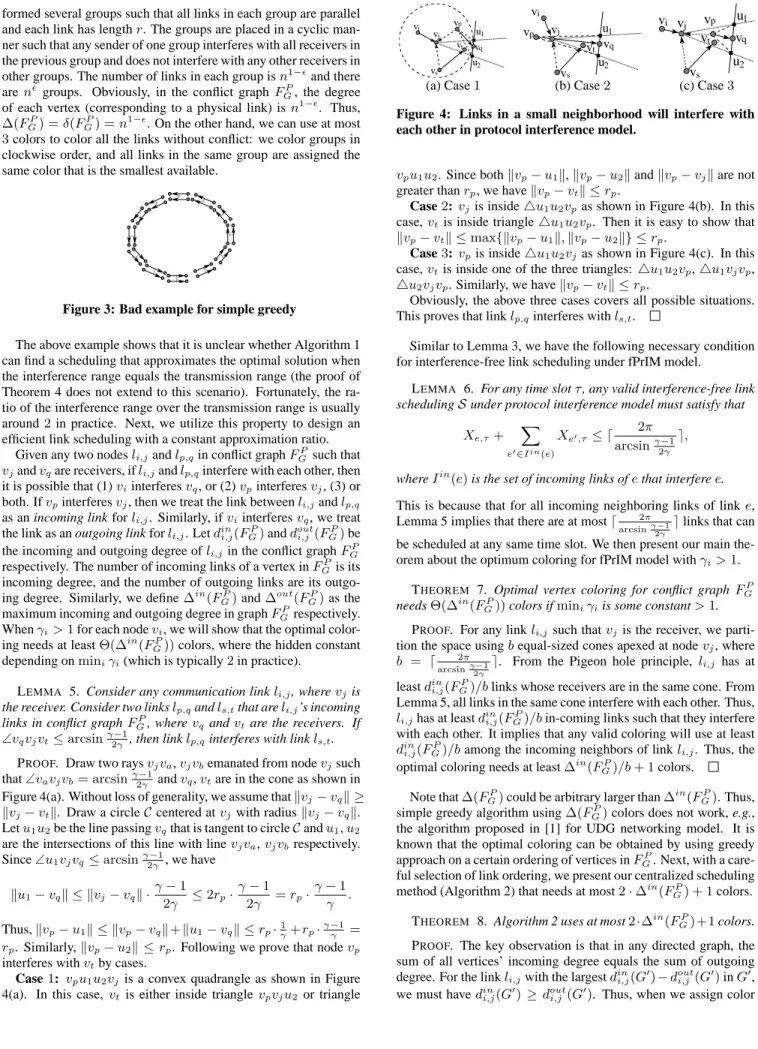
We now describe such an example as in Figure 3. Here all nodes have same transmission range and interference ranger. The links
formed several groups such that all links in each group are parallel and each link has lengthr. The groups are placed in a cyclic man-ner such that any sender of one group interferes with all receivers in the previous group and does not interfere with any other receivers in other groups. The number of links in each group isn1−²
and there aren²
groups. Obviously, in the conflict graphFP
G, the degree of each vertex (corresponding to a physical link) isn1−². Thus, ∆(FP
G) =δ(FGP) =n1−². On the other hand, we can use at most 3colors to color all the links without conflict: we color groups in clockwise order, and all links in the same group are assigned the same color that is the smallest available.
Figure 3: Bad example for simple greedy
The above example shows that it is unclear whether Algorithm 1 can find a scheduling that approximates the optimal solution when the interference range equals the transmission range (the proof of Theorem 4 does not extend to this scenario). Fortunately, the ra-tio of the interference range over the transmission range is usually around2in practice. Next, we utilize this property to design an efficient link scheduling with a constant approximation ratio.
Given any two nodesli,jandlp,qin conflict graphFGPsuch that
vjandvqare receivers, ifli,jandlp,qinterfere with each other, then it is possible that (1)viinterferesvq, or (2)vpinterferesvj, (3) or both. Ifvpinterferesvj, then we treat the link betweenli,jandlp,q as an incoming link forli,j. Similarly, ifviinterferesvq, we treat the link as an outgoing link forli,j. Letdini,j(FGP)anddouti,j(FGP)be the incoming and outgoing degree ofli,jin the conflict graphFGP respectively. The number of incoming links of a vertex inFP
Gis its incoming degree, and the number of outgoing links are its outgo-ing degree. Similarly, we define∆in(FGP)and∆out(FGP)as the maximum incoming and outgoing degree in graphFP
Grespectively. Whenγi>1for each nodevi, we will show that the optimal color-ing needs at leastΘ(∆in(FGP))colors, where the hidden constant depending onminiγi(which is typically2in practice).
LEMMA 5. Consider any communication linkli,j, wherevjis
the receiver. Consider two linkslp,qandls,tthat areli,j’s incoming
links in conflict graphFP
G, wherevq andvt are the receivers. If
∠vqvjvt≤arcsinγ2−γ1, then linklp,qinterferes with linkls,t. PROOF. Draw two raysvjva,vjvbemanated from nodevjsuch that∠vavjvb= arcsinγ2−γ1andvq,vtare in the cone as shown in Figure 4(a). Without loss of generality, we assume thatkvj−vqk ≥ kvj−vtk. Draw a circleCcentered atvjwith radiuskvj−vqk. Letu1u2be the line passingvqthat is tangent to circleCandu1,u2
are the intersections of this line with linevjva,vjvbrespectively. Since∠u1vjvq≤arcsinγ2−γ1, we have
ku1−vqk ≤ kvj−vqk ·γ−1 2γ ≤2rp· γ−1 2γ =rp· γ−1 γ . Thus,kvp−u1k ≤ kvp−vqk+ku1−vqk ≤rp·1γ+rp·γ−γ1 =
rp. Similarly,kvp−u2k ≤ rp. Following we prove that nodevp interferes withvtby cases.
Case1: vpu1u2vjis a convex quadrangle as shown in Figure 4(a). In this case,vt is either inside trianglevpvju2 or triangle
p i vj vs vt u u2 1 q v v v vj u1 u2 vp vi vs vq vt 2 s vi vj vt vq u1 u v vp
(a) Case1 (b) Case2 (c) Case3
Figure 4: Links in a small neighborhood will interfere with each other in protocol interference model.
vpu1u2. Since bothkvp−u1k,kvp−u2kandkvp−vjkare not greater thanrp, we havekvp−vtk ≤rp.
Case2: vjis inside4u1u2vpas shown in Figure 4(b). In this case,vtis inside triangle4u1u2vp. Then it is easy to show that kvp−vtk ≤max{kvp−u1k,kvp−u2k} ≤rp.
Case3: vpis inside4u1u2vjas shown in Figure 4(c). In this case,vtis inside one of the three triangles: 4u1u2vp,4u1vjvp, 4u2vjvp. Similarly, we havekvp−vtk ≤rp.
Obviously, the above three cases covers all possible situations. This proves that linklp,qinterferes withls,t.
Similar to Lemma 3, we have the following necessary condition for interference-free link scheduling under fPrIM model.
LEMMA 6. For any time slotτ, any valid interference-free link schedulingSunder protocol interference model must satisfy that
Xe,τ+ X e0∈Iin(e) Xe0,τ≤ d 2π arcsinγ−1 2γ e, whereIin(e)
is the set of incoming links ofethat interferee.
This is because that for all incoming neighboring links of linke, Lemma 5 implies that there are at mostd 2π
arcsinγ2−γ1elinks that can
be scheduled at any same time slot. We then present our main the-orem about the optimum coloring for fPrIM model withγi>1.
THEOREM 7. Optimal vertex coloring for conflict graphFP G
needsΘ(∆in(FP
G))colors ifminiγiis some constant>1. PROOF. For any linkli,j such thatvjis the receiver, we parti-tion the space usingbequal-sized cones apexed at nodevj, where
b = d 2π
arcsinγ2−γ1e. From the Pigeon hole principle, li,j has at
leastdin
i,j(FGP)/blinks whose receivers are in the same cone. From Lemma 5, all links in the same cone interfere with each other. Thus,
li,jhas at leastdini,j(FGP)/bin-coming links such that they interfere with each other. It implies that any valid coloring will use at least
din
i,j(FGP)/bamong the incoming neighbors of linkli,j. Thus, the optimal coloring needs at least∆in(FGP)/b+ 1colors.
Note that∆(FGP)could be arbitrary larger than∆in(FGP). Thus, simple greedy algorithm using∆(FP
G)colors does not work, e.g., the algorithm proposed in [1] for UDG networking model. It is known that the optimal coloring can be obtained by using greedy approach on a certain ordering of vertices inFP
G. Next, with a care-ful selection of link ordering, we present our centralized scheduling method (Algorithm 2) that needs at most2·∆in(FP
G) + 1colors. THEOREM 8. Algorithm 2 uses at most2·∆in(FP
G)+1colors. PROOF. The key observation is that in any directed graph, the sum of all vertices’ incoming degree equals the sum of outgoing degree. For the linkli,jwith the largestdini,j(G0)−douti,j (G0)inG0, we must havedin
Algorithm 2 Centralized Scheduling under Protocol-Interference
Input: A communication graphG= (V, E)ofmlinks.
Output: An interference-free link scheduling.
1: Construct the conflict graphFGD2and let graphG0=FGD2. 2: whileG0
is not empty do
3: Find the linkli,jwith the largestdini,j(G0)−douti,j(G0)inG0 and remove this vertex fromG0 and all its incident edges. Letlkdenote thekth vertex removed.
4: Process the sequences of linksli,jfromlmtol1. Assign each
linklk the smallest time slot not yet assigned to any of its neighbors inFP
G.
(or time-slot) for the linkli,j, the subgraph induced by all the links that have already been processed is exactly the subgraphG0right before vertexli,j was removed in the while loop of Algorithm 2. Therefore, there are at most2·din
i,j(G0)adjacent neighbors ofli,jin
FP
Gthat have already been processed. In other words, the smallest time-slot assigned toli,jis at most2·dini,j(G0)+1, which is at most 2·din
i,j(FGP)+1. This proves that we need at most2·∆in(FGP)+1 time-slots for an interference-free schedule.
4.
DISTRIBUTED ALGORITHMS
In a wireless network, centralized algorithm may not be possi-ble and even if possipossi-ble, due to the dynamic features of wireless networks, it is inefficient to update the coloring using a centralized algorithm. Thus, in this section, we design efficient distributed al-gorithms to get a valid coloring with good performance guarantee.
4.1
Algorithm For RTS/CTS Model
In literatures, several distributed algorithms have been proposed for the vertex coloring. The first solution is to simply apply a dis-tributed vertex coloring on the conflict graphFD2
G . Recall that all previous distributed algorithms work for the general graph. By tak-ing advantage of special properties of conflict graph defined here, we are able to obtain a deterministic distributed coloring algorithm that colors the links withO(∆(FD2
G ))colors in almost constant time when the interference ranges are homogenous. On the other hand, as shown in our centralized algorithm, the optimal color is Θ(δ(FD2
G ))which could be much smaller than∆(FGD2)when in-terference ranges are heterogenous. Thus, simply applying a col-oring algorithm with ratioΘ(∆(FD2
G ))may not achieve a good performance. The first instinct is to design a distributed version of Algorithm 1. However, finding the node with the global max-imum degree iteratively does not seem promising for distributed algorithm. Thus, we need to find some lower bound for the optimal color other thanO(δ(FD2
G )).
Given two nodesviandvj, we say thatvi precedesvj if and only ifri > rjorri = rjandi > j. Given a pair of linksli,j andlp,qwith different headshi,j6=hp,q, we say thatli,jprecedes
lp,q ifri,j > rp,q orri,j = rp,q andhi,j > hp,q. Recall that
ri,j= max{ri, rj}. We also say that the corresponding vertexli,j precedeslp,qin the conflict graph in this case. For a vertexli,jin graphFGD2, letd≥i,j(F
D2
G )be the number of adjacent vertices that precedeli,j, which is called efficient degree ofli,j. From Theo-rem 2, there are at leastd≥i,j(FGD2)/(2C1)vertices adjacent to and
precedingli,jthat form a clique in which each vertex (i.e., the cor-responding link in the communication graph) interferes with each other. Letφ(FGD2) = maxli,jd
≥
i,j(FGD2), then Theorem 2 shows that optimal coloring algorithm needs at leastφ(FD2
G )/(2C1)
col-ors. Thus, finding a coloring algorithm using at mostΘ(φ(FD2
G )) colors is a constant-ratio approximation algorithm. Unlike the
cen-tralized Algorithm 1 in which the lower bound ofδ(FD2
G )could not be found by using only local information, the lower bound of
φ(FD2
G )could be easily obtained by any linkli,jby simply count-ing the number of interfercount-ing links that precede itself, i.e., with larger link interference radius. Algorithm 3 presents our distrib-uted coloring method that uses at mostφ(FD2
G )colors.
Algorithm 3 Distributed Coloring Algorithm for RTS/CTS Model
Input: A communication graphG= (V, E).
Output: A valid coloring of all links.
1: Each nodevi collects all communication links, sayHi, that containvias the head, i.e., all linksli,jwithri≥rj. 2: Each nodevicollects all communication links, denoted byMi,
that are not inHiand interfere with some linksHi.
3: Nodevi finds Mi+, which is the subset of links inMi that precedes every link inHiand letMi−=Mi−Mi+.
4: Nodevisets all links inMi+as uncolored. 5: while some links inM+
i are uncolored do 6: Nodevilistens messages from other nodes. 7: ifvireceives a messageColor(p, q, k) then
8: Nodevimarkslp,qwith color IDkiflp,qis inMi+. 9: for each nodevjinHido
10: Find the color with minimum color ID, sayk, that is not used by any link that is conflicted withli,j. Color linkli,j with color IDk.
11: Sends the messageColor(i, j, k) to all heads of the links adjacent toli,jinMi−.
THEOREM 9. Algorithm 3 computes a valid coloring using at
mostφ(FD2
G )colors, which is asymptotically optimal.
PROOF. First, we show that the algorithm does terminate. Since it is straightforward that the number of nodes inHiis bounded by
φ(FD2
G ), the for loop terminates inO(n)iterations. Thus, the max-imum time needed for all other processes other than while loop is bounded by a finite timeT and our main focus is to show that the
while loop does terminate for any nodevi. Let(vσ1, vσ2, . . . , vσn)
be the sorted list of nodes in the decreasing order of their interfer-ence range. Thus,vσiprecedesvσj if and only ifi < j. Sincevσ1
precedes every other nodes,Mσ+1is empty andvσ1colors all links
that are adjacent tovσ1in timeT. Now consider the nodevσ2and
M+
σ2. Iflp,q∈M
+
σ2, then eithervporvqisvσ1. Thus, all links in
M+
σ2 are colored. Therefore, all links that are adjacent tovσ2are
colored before time2T. Similarly, all links that are adjacent tovσj are colored before timej·T. Thus, all links are colored in time
n·T. It is straightforward to show that, by assuming color one link takes a unit time, the running time of this algorithm is at mostm, wheremis the number of directed communication links.
Second, we show that the computed coloring is valid, i.e., no two conflict links have the same color. Consider conflict linksli,jand
lp,q, following we discuss by cases.
Case 1:li,jandlp,qhave the same head. Without loss of
gener-ality, we assume thatvi=vpis the head of the links. Thus, both
li,jandlp,qare inHi. Therefore,li,jandlp,qhave different colors.
Case 2:li,jandlp,qhave different heads. Then, without loss of
generality, we can assume thathi,j=i,hp,q=pandviprecedes
vp. Sinceli,j ∈Mp+,li,j is colored beforeMp+ becomes empty. Thus,lp,q is colored afterli,jis. Therefore, whenvpcolorslp,q, it uses a color that is different from the color ofli,j based on our algorithm.
Third, it is straightforward that Algorithm 3 uses at mostφ(FD2
G ) colors, i.e., it has a constant approximation ratio.
Notice that in Algorithm 3, we start to color a link after all in-terfering links preceding it are colored. Thus, in the worst case, it may take timeO(n)to color all the links, wherenis the number of nodes in the network. Here we assume that in one time unit, a node can color all its incident links. Comparing with previous poly-logarithmic time distributed coloring algorithms that color the graph using∆(FGD2) colors, Algorithm 3 may take longer time. However, following example shows that∆(FD2
G )could be as large u1v 1 u2 v2 vi vk ui uk 1 wk wi w2 w
(a) The Original network (b) The Conflict Graph
Figure 5:∆could beΘ(n)of number of colors used by Alg. 3.
asO(n)times of the color used by Algorithm 3, wherenis the number of the nodes in original network. In Figure 5(a), there are
kpairs of transmission linksu1v1, . . . , unvn. Nodesu1, v1have
interference range1and all other nodes have interference range², where²is a small positive constant such that nodeuidoes not in-terferevjfori, j >1. The corresponding conflict graph is shown in Figure 5(b). It is not difficult to see that we only need two colors while the degree ofl1,1isn−1. In other words, compared with
previous poly-logarithmic time methods withΩ(n)approximation ratios, our method has a constant approximation ratio using larger worst-case running time.
4.2
Faster Algorithm For RTS/CTS Model
Although Algorithm 3 computes a coloring that is at most con-stant times of the optimal, it may need linear number of rounds to compute the coloring. In certain circumstances, we would prefer the distributed algorithms that run fast to the distributed algorithms that have good performance as long as the fast distributed algo-rithm does not perform much worse. Following we present another distributed algorithm that computes the coloring very fast with a good performance guarantee ofO(log(ψ) + 1), whereψ is the ratio between the maximum interference range over the minimum interference range among all nodes.
Algorithm 4 Fast Distributed Coloring Algorithm For RTS/CTS
Input: A communication graphG= (V, E).
Output: A valid coloring of the communication graph.
1: Nodevicomputes a subset, sayHi, of all communication links containingvisuch that linkli,j ∈Hiif and only ifri> rj. 2: while nodevifailed to obtain the channel do
3: Nodevimonitors the channel and competes for the channel. 4: for each linkli,j∈Hido
5: Color linkli,jwith the smallest color ID, sayk, that is not used by any link that conflicts withli,j.
6: Broadcasts the messageColor(i, j, k) to each head of links that conflict withli,j.
Algorithm 4 assumes that there is certain competition based MAC layer (e.g., 802.11 with RTS/CTS) available for a node to obtain the channel. We use this MAC mechanism to obtain a link scheduling that is efficient and interference free. Algorithm 4 is very simple and can be implemented without much additional computation on each node. However, the proof of the performance guarantee is not straightforward. To prove the main theorem, we need some
notation in order to extend the Theorem 1 and Theorem 2. For a given node vk, Let N≥(vk, α, β) be a node set composed of the nodes satisfying that (1) each of their interference radius is at least rk
β; (2) each of them interferes some nodes inR(vk, α). Let
N≥(l
i,j, α, β) be the union ofN≥(vi, α, β) and N≥(vj, α, β). The proofs of the following Lemma 10 and 11 are similar to the proofs of Theorem 1 and 2 respectively and thus are omitted here.
LEMMA 10. For any nodevkand any setVk⊆N≥(vk, α, β),
there exists a subsetV0
kofVkwith cardinality at leastd|Vk|/Cα,βe
such that nodes inV0
k interfere with each other whereCα,β = (6αβ+ 1)2+ 11
.
LEMMA 11. For any linkli,jand any setVij⊆N≥(li,j, α, β),
there exists a subsetV0
ijofVijwith cardinality at leatdVij/(2Cα+1,β)e
such that links inVij0 interfere with each other.
Let∆(α, β) = maxli,j|N≥(li,j, α, β)|andχ(FGD2)be the op-timal number of colors. Based on Lemma 11, the following theo-rem is straightforward, for any fixedα, β,
THEOREM 12. χ(FD2
G )≥ d∆(α, β)/(2Cα+1,β)e.
THEOREM 13. Algorithm 4 computes a coloring that is at most
O(log(ψ) + 1)times of optimumχ(FD2
G ).
PROOF. Without loss of generality, let linkli,jbe the link that has the maximum color ID, say g. To prove the theorem, we will show that g ≤ 2C1,2·(log(ψ) + 1)·χ. Following we prove
it by contradiction and for the sake of contradiction, assume that
g>2C1,2·(log(ψ) + 1)·χ.
We first argue that for any0 ≤ k ≤ log(ψ), there exists a linkli(k),j(k)such thatri(k),j(k) < ri,j/2kand its color ID is not smaller than g−2C1,2·k·χ. We prove this argument by
induc-tion onk. Ifk= 0, then the argument trivially holds. Assume for
k ≤p, the argument holds. From Theorem 12, by lettingα= 0 andβ = 2, χ ≥ ∆(0,2)/(2C1,2). In other words, the number
of links, that interfere or are interfered by linkli(p),j(p)and whose
radius is not smaller thanri(p),j(p)/2, is at most2C1,2·χ. Thus,
there must exist a linkli(p+1),j(p+1)such that
1. li(p+1),j(p+1)interferes or is interfered byli(p),j(p);
2. ri(p+1),j(p+1)< ri,j/2p+1; and
3. li(p+1),j(p+1)’s color ID is at least g−2C1,2·(p+ 1)·χ.
This finishes the induction.
Thus, letk = blog(ψ)c, linkliblog(ψ)c,jblog(ψ)c has the color ID not smaller than g−2C1,2· blog(ψ)c ·χ. This implies that
liblog(ψ)c,jblog(ψ)chas at least2C1,2·χ+ 1adjacent links. Since,
ri(blog(ψ)c),j(blog(ψ)c) < ri,j/2blog(ψ)c) andrp,q ≥ ri,j/2log (ψ), all links that interfere or are interfered by linkliblog(ψ)c,jblog(ψ)c have interference radius at leastriblog(ψ)c,jblog(ψ)c/2. From Lemma 11,χ≥ d2C1,2·χ+1
2C1,2 e =χ+ 1, which is a contradiction. Thus,
g≤2C1,2·(log(ψ) + 1)·χ. This finishes the proof.
4.3
Distributed Algorithm Under fPrIM Model
From Theorem 8, any coloring algorithm that usesO(∆in(FGP)) colors under the fPrIM model has a constant approximation ratio. Here we give a distributed algorithm (Algorithm 5) that bears the similar idea of our centralized method (Algorithm 2).
Regarding the distributed method (Algorithm 5), we have: THEOREM 14. Algorithm 5 computes a valid coloring with at
most2·∆in(FP
G) + 1colors withO(m)messages, wheremis the
Algorithm 5 Distributed Scheduling for fPrIM model
Input: A communication networkG= (V, E).
Output: A valid coloring of all links.
1: Assign each communication link a label WHITE.
2: The header of each communication linkli,jcollects all incom-ing links and outgoincom-ing links, denoted byMin
i,jandMi,jout. 3: while linkli,jis WHITEdo
4: Linkli,jmonitors the channel. 5: If some linkeinMin
i,j
S
Mout
i,j announces that it becomes GRAYwith time-stampk, linkli,jlocally stores the label of linkeas GRAYand the time stampk.
6: if the number of WHITElinks inMin
i,jis not smaller than the number of WHITElinks inMout
i,j then 7: Linkli,jcompetes for the channel.
8: if Linkli,jobtains the channel then
9: Linkli,j labels itself GRAYwith a time stampt+ 1 wheretis the maximum time stamp of all GRAYlinks stored locally. Heret= 0is no GRAYlinks are stored. Linkli,jsend to all adjacent links inFGP the message thatli,jbecomes GRAYwith the time stampt+1. Link
li,jmakes a list of linksSi,jcomposed of the current WHITElinks inMin
i,j
S
Mout i,j .
10: while there exists some links inSi,jnot colored do
11: Linkli,j listens to the announcement. If a linke0 in Si,j announces its color, then linkli,j locally updates the status ofe0
as colored together with the color ofe0
.
12: Linkli,j colors itself using the smallest color available that will not produce any conflict with links inSi,j. It then sends to all adjacent links inFP
G without a color the message about its current color assigned.
PROOF. Notice that for each linkli,j, it uses the smallest color that is not used by any links inSi,j. Since the number of incom-ing links is not smaller than the outgoincom-ing links inSi,j, linkli,jis colored with a color not greater than2·din
i,j(FGP) + 1. Thus, Al-gorithm 5 computes a valid coloring with at most2·∆in(FP
G) + 1 colors. Note that each linkli,jonly announces twice in our distrib-uted scheduling algorithm: when it becomes GRAYand when it is colored. Thus, the overall message complexity isO(m).
5.
WEIGHTED COLORING AND
SCHEDU-LABLE FLOWS
5.1
Scheduling With Traffic Load
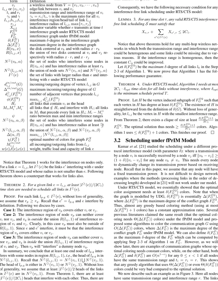
In TDMA system, the minimization of the number of colors is closely related to the maximization of the network throughput. One intrinsic assumption behind the idea of coloring is that each com-munication link has the same packet arrive rate, i.e., the number of traffics that need to go through each communication link is same. However, this is not likely to be true and it is possible that some communication link carries more traffic than others.
t
1s
is
kt
1t
2s
is
2t
k 1v
v
2 k 1s
is
kt
1t
2t
is
2t
k 2 1 1 2 i k k+1 2 is
1v
v
(a) network (b) assigned colors
Figure 6: Simple example: unweighted coloring is inefficient.
Consider a simple example of multihop wireless network com-posed ofksource and destination pairs(si, ti)as shown in Figure 6(a). For simplicity of our presentation, we assume that every node in the network can transmit atabps if it uses all time slots. Observe that we need at leastk+ 1colors, which can be obtained by assign-ing colorito linkssiv1andv2ti, and colork+ 1to linkv1v2as in
Figure 6(b). This implies that communication linkv1v2can
trans-mit once everyk+ 1time slots. However, the path between each source destination pair needs to go through linkv1v2. Thus, link
v1v2becomes the bottleneck and the overall network throughput is
only k+1a bps. For each source destination pair, its throughput is approximately k·(ka+1) bps, which is inefficient. Thus, we need to generalize the coloring that can take the traffic rate on each com-munication link into account. In this paper, we use the weighted
coloring to capture this, which is defined as follows.
DEFINITION 1. Given a graphG= (V, E)whereV is the set of vertices andE is the set of links. Every linkei ∈ E has an
integral weightwi≥0. A weighted link coloring is an assignment
of at leastwidistinct colors to each linkeisuch that no two links
sharing the same color interfere with each other.
By introducing the notation of weighted coloring, we can as-sign different weight to different communication links. For ex-ample, given a set ofk flow requirementsfifromsitoti, 1 ≤
i≤k, a certain routing algorithm will determine the routing path for each flow. The weight of a linkeis then the total flow pass-ing throughP edivided by the bandwidthc(e)of linke, i.e.,we =
fi:fi using efi
c(e) . Let us see how the weighted coloring can help to
improve the throughput using the example shown in Figure 6. By assigning weight1to each linksiv1,v2tifor1 ≤i ≤ kandk tov1v2, obviously a valid2kcoloring can be obtained. It is not
difficult to observe that the total throughput is nowa/2bps and each communication pair has a throughput ofa/2k. This increases the throughput obtained from the unweighted coloring by an order ofk. Following, we show how to obtain a valid weighted coloring based on the unweighted coloring.
Algorithm 6 Weighted Coloring Algorithm Based on Unweighted
Coloring AlgorithmA
Input: A communication graphG= (V, E)with weight on each
link and an unweighted coloring algorithmA.
Output: A valid coloring of the links.
1: Build the conflict graphFGbased on original graphGand interference model. Assign weightwi,jto vertexli,j∈FG. 2: Construct a new conflict graphF0
GfromFGas follows: for each vertexli,jwith weightwi,j, we createwi,jvertices,l1i,j,
l2
i,j,. . .,l wi,j
i,j and add them toFG0. Add to graphFG0 the edges connectingla
i,j,lbi,jfor1≤a < b≤wi,j. Add to graphFG0 an edge betweenlai,j andlbp,q if and only if there is an edge betweenli,jandlp,qin graphFG.
3: Run the unweighted vertex coloring algorithmAonF0
G. 4: Assign linkli,jall the colors that are used bylki,jfor1≤k≤
wi,jinFG0.
We then show that Algorithm 6 has a performance guarantee that is not worse than that of the unweighted coloring algorithmA.
THEOREM 15. IfAuses at mostαtimes of the optimal colors for unweighted coloring, then Algorithm 6 also needs at mostα times of the optimal colors for weighted coloring.
PROOF. Notice that for any valid weighted coloring forFG,li,j is assigned at leastwi,jcolors. By assigning each vertexlki,jinFG0 a distinct color that is assigned toli,j, we obtain a valid unweighted coloring forFG0. Thus, χ(FG0) ≤ χ(FG). Hereχ(FG0) is the minimum number of colors needed for unweighted coloring inF0
G andχ(FG) is the minimum number colors needed for weighted coloring inFG. SinceAwill return a coloring with at mostα·
χ(F0
G)colors, Algorithm 6 produces a coloring with at mostα·
χ(F0
G)≤α·χ(FG)colors. This finishes the proof.
The basic idea of Algorithm 6 is to create a clique of sizewi,j for each linkli,jand color the new graph using unweighted color-ing methodA. Although this gives a general framework to design weighted coloring, its time-complexity could be large if the weight is large. Fortunately, Algorithm 6 could be simplified without much overhead compared to the unweighted algorithm: the main idea is to assign colors for one link at once: instead of assigning one time-slot to a linklk, we assignwktime-slots to linklk when process linklk. As an example, we modify the Algorithm 4 to obtain a fast weighted coloring (Algorithm 7). Following we show that Algo-rithm 7 has the same performance guarantee as AlgoAlgo-rithm 4.
Algorithm 7 Fast Distributed Weighted Coloring Algorithm
Input: A communication graphG= (V, E).
Output: A valid coloring of links in the communication graph.
1: Nodevicomputes a subset, sayHi, of all communication links containingvisuch that linkli,j ∈Hiif and only ifri> rj. 2: while nodevifailed to obtain the channel do
3: Nodevimonitors the channel and competes for the channel. 4: for each linkli,j∈Hido
5: Color linkli,j with the first fitwi,j colors that are not used by any link that interferes or is interfered byli,j. Here, the assigned colors are not requi