An International Comparison of Implied, Realized and GARCH Volatility Forecasts

1

An International Comparison of Implied,

Realized and GARCH Volatility Forecasts

*

Apostolos Kourtis, Raphael N. Markellos and Lazaros Symeonidis

Abstract

We compare the predictive ability and economic value of implied, realized and GARCH

volatility models for 13 equity indices from 10 countries. Model ranking is similar across

countries, but varies with the forecast horizon. At the daily horizon, the Heterogeneous

Autoregressive model offers the most accurate predictions while an implied volatility model

that corrects for the volatility risk premium is superior at the monthly horizon. Widely used

GARCH models have inferior performance in almost all cases considered. All methods perform

significantly worse over the 2008-09 crisis period. Finally, implied volatility offers significant

improvements against historical methods for international portfolio diversification.

JEL codes: G15; G17; G01; G11

Keywords: Implied Volatility; Realized Volatility; Volatility Risk Premium; Financial Crisis;

International Diversification

*_{We would like to thank two anonymous referees, the editor Robert Webb, Marcel Prokopczuk, Chardin Wese}

Simen and the participants at the 9th _{International Conference on Computational and Financial Econometrics for}

useful comments and suggestions. Part of this project was completed when Symeonidis was a postgraduate researcher at the ICMA Centre, University of Reading.

† _{Norwich Business School, University of East Anglia, Norwich NR4 7TJ, UK. Contacts: Apostolos Kourtis:}

a.kourtis@uea.ac.uk, Tel.: +44(0)1603591387, Raphael Markellos (corresponding author): R.Markellos@uea.ac.uk, Tel.: +44 (0)1603597395, Fax: +44 (0)1603593343, Lazaros Symeonidis:

2

1.

Introduction

Volatility is a key concept in finance especially in portfolio selection, option pricing and risk

management. Despite a variety of shortcomings and alternatives, volatility still lies at the heart

of modern finance. It is not surprising that a vast methodological and empirical literature exists

around the development, assessment and application of volatility forecasts.

Unfortunately, it

is difficult to draw clear conclusions from the existing literature as research designs vary

considerably across different studies in terms of: countries, asset classes, time periods,

forecasting techniques, forecast horizons and forecast evaluation methods. Our study aims to

overcome this difficulty by comparing some of the most popular volatility models within a

common framework. Our analysis employs 13 equity indices from 10 countries, three forecast

horizons and different market conditions, i.e. before, during and after the 2008-09 crisis.

Comparisons between models are performed on the basis of different statistical tests and loss

functions. Most importantly, we assess the economic significance of the competing volatility

forecasting models within an international portfolio choice framework.

The models we consider span the three most prominent families of volatility forecasting

methods. First, we have the GJR-GARCH of Glosten et al. (1993) which descends from the

ARCH family of historical volatility models. We select this model on the basis of its popularity

amongst academics and practitioners and the fact that it is often found to have superior

performance against alternative ARCH specifications (e.g., see Brownlees et al., 2012).

Second, we use two model specifications based on raw and volatility risk-premium adjusted

implied volatility levels, respectively. For the adjustment we use the technique of Prokopczuk

and Wese Simen (2014) which reduces the bias in the raw implied volatility. It is the first time

a study assesses the importance of adjusting for the volatility risk premium in volatility

forecasting in the context of international equity markets. Third, we employ realized

volatility-based forecasts using plain lagged values and the Heterogeneous Autoregressive (HAR) model

of Corsi (2009). The latter approach is becoming increasingly popular due to its simplicity and

modeling accuracy (e.g., see Giot and Laurent, 2007; Corsi et al., 2010; Busch et al., 2011;

Patton and Sheppard, 2015).

We adopt the standard practice of using the daily realized volatility as a proxy for the

“actual” latent volatility. We then employ a battery of different techniques in order to compare

the volatility models on the basis of various statistical and economic criteria. In order to

1 _{Characteristically, on 24 November 2015, 6,110 papers in Google Scholar and 1,548 research outputs in Scopus}

3

accommodate the possibility of different forecasting scenaria and tasks, we use horizons of 1,

5 and 22 days, respectively. We apply univariate Mincer-Zarnowitz as well as encompassing

regressions to assess the information content of each set of volatility forecasts in an in-sample

setting. Out-of-sample analysis is based on the Diebold-Mariano test of predictive accuracy.

Two statistical loss functions are utilized: the root mean-squared error and the quasi-likelihood.

We perform several robustness checks by considering alternative models, configurations and

estimation periods along with the effect of volatility spillovers from the US.

We find that model rankings remain roughly the same across countries but vary with the

forecast horizon. While the results for the weekly horizon are mixed, the HAR model is

superior at the daily horizon and the implied volatility model yields the best forecasts at the

monthly horizon. The superiority of the volatility risk premium-adjusted implied volatility

forecasts at the monthly horizon is likely due to the fact that all model-free implied volatility

indices have a fixed forecast horizon of one month by construction. Our results also reveal that

volatility risk premium-adjusted implied volatility forecasts outperform raw implied volatility

forecasts in most markets under consideration. This finding highlights the importance of

accounting for the volatility risk premium when forecasting volatility using information from

option prices. In line with the literature, comparing raw implied volatility forecasts to lagged

realized volatility forecasts leads to mixed results (see Blair et al., 2001; Jiang and Tian, 2005;

Pong et al., 2004; Martens and Zein, 2004; Andersen et al., 2007b). Finally, we find that the

historical GJR-GARCH model underperforms the realized and implied volatility alternatives

in almost all cases (similar results are reported by Flemming, 1998; Jorion, 1995; Andersen et

al., 2003; Covrig and Low, 2003; Giot, 2003; Andersen et al., 2007b and Charoenwong et al.,

2009, among others).

Accurate volatility predictions are particularly important during periods of market turmoil,

such as that of 2008-2009, when risks typically soar (see Schwert, 2011). Given that our dataset

spans the period 2000-2012, we examine whether the performance of our forecasting methods

changes between periods of market calmness and unrest. The ranking of our models is

comparable in the periods before, during and after the crisis. However, all models perform

significantly worse during the crisis period. This result suggests that researchers and

practitioners should be more cautious when forecasting volatility during periods of market

downturn.

Finally, we examine the practical value of the forecasting models considered for an

international investor. This reveals that implied volatility-based forecasts lead to superior

out-of-sample portfolio performance. In particular, only this forecasting method yields portfolios

4

that manage to outperform our benchmark strategy of an equally-weighted portfolio (1/N). We

also find that correcting for the volatility risk premium further improves portfolio performance.

The remainder of the paper is organized as follows. Section 2 presents our data and the

forecasting models under consideration. The information content and predictive ability of the

models is evaluated in sections 3 and 4, respectively. Section 4 also examines the value of the

volatility forecasts before, during and after the 2008-09 crisis period. Section 5 assesses the

economic value of volatility forecasts. Section 6 summarizes our robustness checks while the

last section concludes the paper.

2.

Methodology

2.1

Data

Our analysis involves three types of data. First, we collect daily dividend-adjusted closing

levels for 13 international equity indices from Bloomberg. We use these to compute percentage

index returns. Second, we use a daily realized volatility series for each equity index,

constructed from equally spaced 5-min intraday returns. These series are collected from the

Oxford-Man Institute Realized Library of the University of Oxford. Finally, we obtain daily

data on the option implied volatility indices which correspond to the equity markets under

consideration, from Bloomberg. All implied volatility indices used are constructed in a

model-free manner. Our sample spans the period from January 3, 2000 to October 26, 2012, although

for some markets the sample is shorter. Table 1 reports the equity indices considered, along

with the sample period covered and the relevant implied volatility indices.

2.2

Volatility Forecasting Models

This section describes our proxy of the actual unobserved volatility and the volatility

forecasting models we use in our analysis, respectively.

2.2.1

Realized Volatility

As the true volatility is unobservable, we need to proxy it using an observable variable. The

most popular and theoretically appealing proxy is the so-called realized variance. This is given

by the sum of squared intraday returns sampled at equally spaced intervals (see Andersen and

Bollerslev, 1998; Barndorff-Nielsen and Shephard, 2002b). It has been shown that in a

5

frictionless market realized variance is a consistent estimator of the actual unobserved variance

(Barndorff-Nielsen and Shephard, 2002a). In particular, it follows from the quadratic variation

theory that realized variance asymptotically converges to the actual unobserved variance as the

sampling frequency increases to infinity.

Suppose that on a trading day

t,

we observe

M+1

prices at times:

𝑡

, 𝑡

, 𝑡

, … , 𝑡

. If

𝑝

is

the logarithmic price at time

𝑡

, then the corresponding return,

𝑟

, for the

𝑗

intraday interval

of day

t

is defined as:

𝑟

= 𝑝

− 𝑝

. The

realized volatility

estimator for day

t

is then defined

as the square root of the sum of squared intraday returns:

𝑅𝑉

= √∑

𝑟

𝑗

2 𝑀

𝑗=1

(1)

Realized volatility over horizons of

k

days is given by

𝑅𝑉

= √∑

𝑅𝑉

, under the

convention that

𝑅𝑉

=

𝑅𝑉

. In our analysis, we consider horizons of 1, 5 and 22 days,

respectively.

2.2.2

Forecasts from Intraday Returns (LRE)

The first forecasting model we consider involves the lagged realized volatility (LRE). This

model stems from the assumption that volatility is a Markov process and therefore last period’s

volatility is highly informative of future values. An alternative to LRE would be to use

historical volatility constructed from daily data. Nevertheless, extensive empirical evidence has

shown that historical volatility estimators obtained using daily data are inferior to

high-frequency-based counterparts (e.g., Andersen and Bollerslev, 1998; Blair et al., 2001, Andersen

et al., 2007a).

2.2.3

Model-Free Implied Volatility Forecasts (MFIV)

The second forecasting model we adopt is based on volatility measures implied from the prices

of liquid traded options. Option implied volatility can be constructed using the Black-Scholes

(BS) option pricing model. However, this approach fails to accommodate empirically

documented facts, such as stochastic volatility, non-Gaussian returns, etc. To address these

issues, recent research advocates the derivation of implied volatility in a model-free manner

that employs mid-quote prices of out-of-the money call and put options with different strike

6

prices and maturities (e.g., Britten-Jones and Neuberger, 2000). The implied volatility indices

we adopt in this work are constructed this way.

Implied volatility indices represent the market expectation of future volatility of the

underlying equity index over the next 30 calendar days. In order to predict volatility at various

horizons, we re-scale implied volatility so that it forecasts the

k

-day volatility (see for example,

Blair et al., 2001). This is done by setting

𝑀𝐹𝐼𝑉

= √

252

𝐼𝑉

, where:

𝐼𝑉

is the daily value

of the implied volatility index. Then,

𝑀𝐹𝐼𝑉

corresponds to the

k

-day option implied

volatility forecast.

2.2.4

Model -Free Implied Volatility Adjusted for the Volatility Risk Premium

(C-MFIV)

It is well known that implied volatility is a biased estimator of future volatility (Jiang and Tian,

2005; Andersen et al., 2007b). One of the main reasons for this bias is the existence of an

economically significant variance risk premium (see Chernov, 2007). To correct for this

premium, Prokopczuk and Wese Simen (2014) introduce a simple non-parametric adjustment

to the implied volatility in their study of energy futures markets. They show that accounting

for the volatility risk premium leads to superior volatility forecasts, compared to time series

models, Black-Scholes implied volatility and the non-adjusted MFIV.

Motivated by this evidence, we assess the value of the approach of Prokopczuk and Wese

Simen in the context of equity markets. In particular, we consider a relative variance risk

premium, defined as:

𝑉𝑅𝑃

= 𝐸

(𝑉𝑎𝑟

)/𝐸

(𝑉𝑎𝑟

)

,

(2)

where

P

and

Q

are the physical and risk-neutral probability measures, respectively, and

𝑉𝑎𝑟

is the variance from day to

t

to day

t+k

. Empirically, the risk neutral expectation of

variance between

t

and

t

+

k

can be estimated using

𝑀𝐹𝐼𝑉

. To estimate the ex-ante

expectation of variance under the physical measure, we employ the realized variance computed

from 5-min. intraday returns. Then, following Prokopczuk and Wese Simen (2014), the average

estimated relative variance risk premium over a period of 252-

k

days is:

𝑉𝑅𝑃

̅̅̅̅̅̅

=

1

252 − 𝑘

∑

𝑀𝐹𝐼𝑉

𝑅𝑉

,

(3)

7

where

k

is the forecast horizon (

k

=1, 5 or 22). Finally, the

corrected model-free implied

volatility

(

C-MFIV

) forecast for a horizon of

k

days is obtained as follows:

𝐶 − 𝑀𝐹𝐼𝑉

=

𝑀𝐹𝐼𝑉

√𝑉𝑅𝑃

̅̅̅̅̅̅

. (4)

Other approaches in the literature that correct for the variance risk premium include

Chernov (2007) and Kang et al. (2010). Chernov relies on at-the-money option contracts and

models the volatility risk premium as an affine function of the underlying spot volatility. Kang

et al. take a more structural approach that employs investor risk preferences and higher order

risk neutral moments. While both of these alternatives successfully correct for the variance risk

premium, we adopt the technique of Prokopczuk and Wese Simen, as it is simpler to apply in

our framework without requiring additional estimations from options data. Moreover, as

argued by Prokopczuk and Wese Simen, dividing raw implied volatility by the squared root of

the variance risk premium, instead of using a volatility spread as in Chernov, can improve

volatility forecasting in time-periods that include regime switches. This makes the method of

Prokopczuk and Wese Simen more suitable for our empirical analysis, as our datasets cover

the 2008-09 financial crisis. A potential downside of (4) is that the choice of the averaging

period is not theoretically justified. To deal with this issue, we consider alternative estimation

periods, namely 18 and 24 months, and we do not observe any significant change in our results.

2.2.5

GJR-GARCH Model Forecasts (GJR)

The fourth forecasting model in our analysis is the so-called GJR-GARCH model of Glosten

et al. (1993). This captures serial dependencies in an asymmetrical manner in that negative

shocks have a greater impact on volatility than positive shocks of the same magnitude.

Moreover, if offers superior forecasting performance against other ARCH specifications (see,

for example, Brownlees et al., 2012). The GJR-GARCH model is specified as follows:

ℎ

= 𝜔 + 𝛼 𝑒

+ 𝛾 Ι

𝑒

+ 𝛽 ℎ

, (5)

where

𝑒

are the residuals from the mean equation

𝑟

= 𝜇 + 𝑒

,

𝜇

is the unconditional mean of

the return series,

ℎ

is the conditional variance of the residuals and

Ι

is an indicator

8

produce out-of-sample volatility forecasts, we estimate the above model on a rolling basis using

a window of 800 observations and construct

k

-step ahead forecasts in a recursive manner.

2.2.6

Heterogeneous Autoregressive Model Forecasts (HAR)

The literature highlights the importance of long memory for modelling and forecasting

volatility (Comte and Renault, 1998; Areal and Taylor, 2002; Andersen et al., 2003; Deo et al.,

2006). Alas, many of the conventional long memory models, such as the Fractional Integrated

GARCH (FIGARCH), present significant estimation and computational difficulties. To

overcome such issues, we adopt the Heterogeneous Autoregressive (HAR) model introduced

by Corsi (2009). This is relatively straightforward to estimate and can capture known stylized

facts of financial data, such as long memory and fat tails.

In the HAR setting, realized volatility over the next

k

days is modeled as an affine function

of past realized volatilities computed over three different horizons:

𝑅𝑉

= 𝜔 + 𝛽

𝑅𝑉

+ 𝛽

𝑅𝑉

+ 𝛽

𝑅𝑉

+ 𝑒

(6)

To be consistent with the application of the GJR-GARCH model, we estimate the above model

using a rolling sample of the 800 most recent observations. We then use the parameter estimates

to forecast the volatility of equity returns over horizons of 1, 5 and 22 business days,

respectively.

3.

Information Content of Volatility Forecasts

3.1

Univariate Regressions

To assess the information content of individual volatility forecasts we estimate

Mincer-Zarnowitz regressions (Mincer and Mincer-Zarnowitz, 1969). These involve regressing the

k-

day

realized volatility for each equity index on forecasts from the different volatility models:

𝑅𝑉

= 𝛼 + 𝛽 𝐹̂

+ 𝑒

, (7)

where

𝐹̂

is the

k

-day ahead forecast from a particular volatility forecasting model. A

forecast is informative about future volatility if it has a coefficient in regression (7) that is

statistically different from zero.

9

The results from estimating the above regressions are reported in Tables 2 and 3 for the

daily and monthly horizon, respectively (to preserve space, results for the weekly horizon can

be found in the Appendix A). The tables give the coefficient estimates (

𝛽

) for each forecasting

model along with the associated

t

-statistics in parentheses. The bottom section of each table

presents the average values of the coefficients for each forecasting model across the thirteen

indices. We observe that all slope coefficient estimates are statistically significant, indicating

that all forecasts bear information about future volatility. Looking at the results across markets,

we observe that according to the adjusted

𝑅

(𝑅̅

) values the HAR model has the greatest

explanatory power at the daily horizon for 9 out 13 indices. However, at the monthly horizon

the C-MFIV model exhibits the highest

𝑅̅

values in 12 out of 13 markets. At the weekly

forecast horizon, the results are more mixed with the GJR, HAR and MFIV producing the most

informative forecasts in the majority of markets. Notably, the GJR model is superior for the

S&P 500 index for all three forecast horizons considered.

Regression (7) can also be employed to assess the biasedness of volatility forecasts. In

particular, a volatility forecast is an unbiased forecast of future realized volatility, if

𝛼 = 0

and

𝛽 = 1

. We test the validity of this joint restriction through a standard Wald-type test. As we

use overlapping samples, the errors from (7) are serially correlated for forecasting horizons that

exceed one day. For this reason, we employ the heteroscedasticity and autocorrelation

consistent standard errors of Newey and West (1987) with

k

lags. We draw three conclusions

from these results which are available upon request. First, for most markets and forecast

horizons the regression intercept

α

is statistically significant while

β

is different from 1. This

result means that most volatility forecasts are biased and is in line with Jiang and Tian (2005)

and Andersen et al. (2007b). The only notable exception is the HAR model at the 1-day forecast

horizon where the restriction cannot be rejected for 6 out of the 13 equity markets at the 5%

significance level. Second, the observed bias is significantly smaller for the HAR forecasts and

to a lesser extent for the C-MFIV forecasts, respectively. Third, our results indicate that the

volatility risk premium adjustment significantly reduces the bias in the model-free implied

volatility. The reduction is more pronounced at the monthly forecast horizon.

3.2

Encompassing Regressions

We further assess the incremental information content of the volatility forecasts by estimating

encompassing regressions for each of the 13 equity markets. These regressions replace the

individual forecasts in the right hand-side of (7) with a pair of forecasts from competing

10

volatility models. Apart from the relative importance of two competing volatility forecasts,

encompassing regressions can detect whether a volatility forecast subsumes all the information

included in another forecast.

Table 4 presents aggregate results for daily and weekly encompassing regressions, namely,

the average intercept and slope as well as the average

𝑅̅

coefficient across the thirteen indices.

Extensive results for daily and weekly forecasts are not reported, as they indicate that all

forecasting models contain information about future volatility with statistically significant

coefficients at the 5% level. We find that all models explain a large fraction of the variation in

realized volatility, since the average

𝑅̅

values range between 70.7% (74.2%) and 72.7% (75%)

at the daily (weekly) forecast horizon.

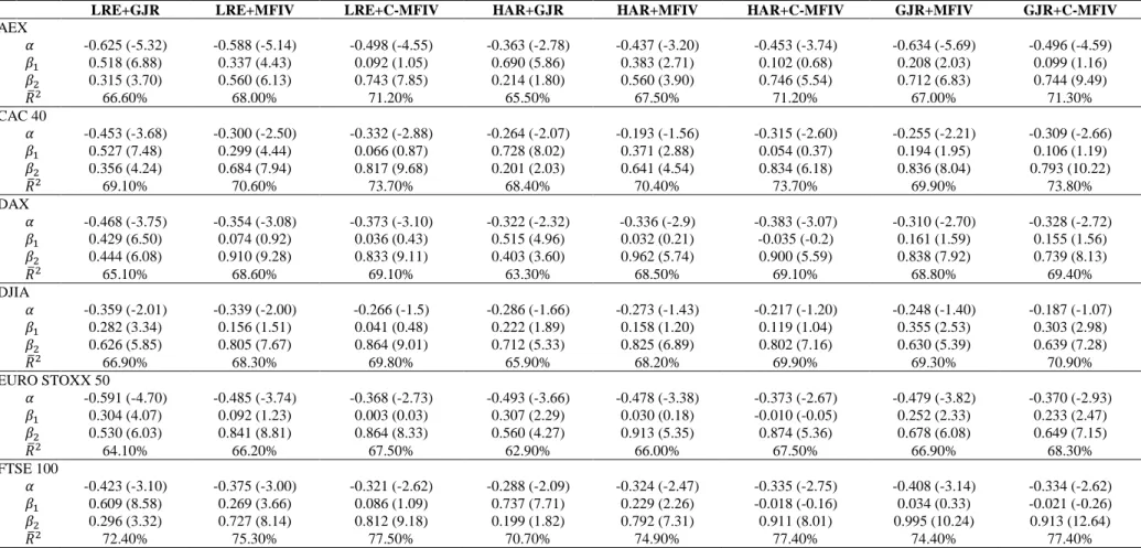
More interesting results emerge from the monthly encompassing regressions presented in

Table 5. First, focusing on the fourth column of the table (labeled “LRE+C-MFIV”) reveals

that the corrected model-free implied volatility subsumes all information contained in lagged

realized volatility. The coefficients of C-MFIV are all highly significant and lie between 0.70

and 0.99. In contrast, the raw MFIV is not significantly superior to lagged realized volatility.

This result confirms the importance of accounting for the volatility risk premium for volatility

forecasting. Second, C-MFIV subsumes the information in HAR forecasts in all markets except

for the S&P 500. The raw MFIV also outperforms HAR forecasts in 7 out of 13 markets. Third,

C-MFIV yields superior forecasts to GARCH in 6 of the 13 markets (see column labeled

“GJR+C-MFIV”), while for the remaining markets both are informative, but C-MFIV has a

more pronounced impact on realized volatility as indicated by the greater regression

coefficients. The latter result extends to all regressions that involve raw or adjusted implied

volatility, indicating that these models have a stronger effect on future volatility compared to

the remaining models. This finding is also clear from the bottom panel of Table 5, which

contains the cross-sectional average of the regression coefficients.

Overall, our results indicate the superiority of implied volatility forecasts in the monthly

horizon. The superior predictive ability of the C-MFIV at the monthly horizon is likely a

consequence of its construction from options with maturity of one month. This is in line with

Taylor et al. (2010) who show that option implied volatility forecasts are more informative than

3 _{We do not present combinations of in-sample forecasts for CMFIV+MFIV and LRE+HAR in Tables 4 and 5.}

The main reason is that the MFIV is essentially nested within the C-MFIV and LRE is nested within HAR. Moreover, from an econometric perspective, inclusion of MFIV (LRE) and the C-MFIV (HAR) in the same regression would make it much more susceptible to multicollinearity.

11

historical volatility when the forecast horizon matches the maturity date of the underlying

options.

In summary, the results from univariate and encompassing regressions suggest that all

forecasts are informative about future volatility across all markets, even though they generally

produce biased forecasts. The forecast horizon determines the most informative model with the

HAR and the C-MFIV being clearly superior at the daily and monthly horizons, respectively.

4.

Out-of-Sample Forecast Evaluation

So far, our analysis has been devoted to regressions that explore the information content of

volatility forecasts in-sample. In this section, we assess the out-of-sample forecasting accuracy

of the competing models. To this end, we consider two of the most frequently used loss

functions: the root mean squared error (RMSE) and the quasi-likelihood (QLIKE). These are

defined as:

𝑅𝑀𝑆𝐸 = √

1

𝑁

∑(𝑅𝑉

− 𝐹̂

)

(8)

𝑄𝐿𝐼𝐾𝐸 =

1

𝑁

∑ [log (𝐹̂

) +

𝑅𝑉

𝐹̂

]

, (9)

where

N

is the number of out-of-sample volatility forecasts. RMSE is a popular choice in

empirical applications while QLIKE is known to be robust to noise in the volatility proxy

(Patton, 2011).

To formally investigate whether the differences between the forecast errors of competing

volatility models are statistically significant, we employ the Diebold-Mariano (DM) predictive

accuracy test (Diebold and Mariano, 1995). In implementing the DM test, we account for

possible autocorrelation in overlapping multi-period forecasts using the covariance estimator

of Newey-West (1987).

Tables 6 and 7 report our out-of-sample results (results for the weekly forecast horizon are

reported in Table A2 of the appendix to save space). Rows correspond to markets and columns

correspond to forecasting models. Panel A (Panel B) reports the results for the RMSE (QLIKE)

loss function. The model with the lowest forecast errors for each loss function is highlighted in

bold. Models with significantly higher forecast errors than the best model according to the DM

12

test at the 5% (10%) are marked with two (one) asterisks. The results generally indicate model

rankings that are similar to those obtained previously by the in-sample univariate and

encompassing regressions. Starting with Table 6, we observe that HAR is clearly the best

performing model at the daily horizon. All models are inferior to the HAR model, according to

both performance criteria. The model with the worst overall performance is the MFIV, which

yields the highest forecast error in almost all markets, followed by the GJR-GARCH. For

instance, in the case of the NASDAQ index, HAR has a RMSE value of 0.29, while at the same

time the RMSE of MFIV is more than double as high and equal to 0.69.

Table 7 shows that at the monthly horizon C-MFIV exhibits the lowest forecast errors

among almost all competing models for all markets and loss functions. The loss differences of

most models against the C-MFIV are statistically significant at the 5% level. The only

exception is the HAR model. Nevertheless, HAR still has larger forecast errors than C-MFIV

for the majority of the markets. HAR also appears to outperform the raw implied volatility

forecasts in all markets according to both criteria. The GJR-GARCH model underperforms

most of the models except for the MFIV. The latter results shows that correcting implied

volatility for the volatility risk premium is of high importance when forecasting volatility.

The results for the weekly horizon suggest that C-MFIV produces the lowest forecast errors

for the majority of the markets (Table A2 in appendix). In particular, according to the RMSE

(QLIKE), C-MFIV yields the best performance in 10 (8) out of 13 markets. Nevertheless, the

differences in forecast errors between C-MFIV and HAR are insignificant in all but 2 cases.

Again MFIV and GJR-GARCH result in the worst performance. For example, we find that the

RMSE value for C-MFIV is 0.46 compared to a 0.98 for GJR-GARCH in the FTSE 100 index.

We further investigate whether the accuracy of volatility forecasting changes in periods of

market turmoil. In this context, we perform a separate out-of-sample forecast evaluation over

three different sub-periods: (i) the pre-crisis period (January 2003- July 2008), (ii) the crisis

period (August 2008-December 2009) and, (iii) the after-crisis period (January 2010 – August

2012). We define the crisis period to be the shortly after the Lehman collapse until the end of

2009, similar to Genre et al. (2013).

Tables 8-9 present forecast losses for each market and

forecasting model over the three sub-periods considered (weekly results are in Table A3 of the

appendix to conserve space).

4 _{We have experimented with different periods such as 2007-2009 and obtained almost identical results. These}

13

This analysis leads to three major conclusions. First, the forecasting ability of all models

significantly deteriorates over the crisis period according to both loss functions. Also for most

markets, the forecast errors in the post-crisis period are higher than the errors in the pre-crisis

period. One of the possible explanations for this is the anomalous situation around European

sovereign debt in the post-crisis period. These results indicate that academics and practitioners

should be more cautious when forecasting volatility in periods of turmoil. Second, as in the full

sample, HAR and C-MFIV are superior to the remaining models during the crisis period, at the

1-day and 22-day horizons, respectively. Although model rankings do not change for these

horizons, the statistical differences among models are less significant. Third, the ranking of the

models at the weekly horizon substantially changes in the crisis period and the evidence

regarding the best model is fairly mixed. However, the loss differences between the best models

are almost never statistically significant.

5.

Economic Value of Volatility Forecasts

We now assess the economic value of the five volatility forecasting methodologies under study

from the perspective of an international portfolio investor. We consider a market of 11 assets,

which correspond to 11 out of the 13 international indices we consider. We exclude KOSPI

and Russell 2000 from this analysis due to the relatively smaller period that their data span.

We also do not account for currency risk, as this goes beyond the aims of this study. We assume

weekly and monthly rebalancing instead of daily to avoid any significant bias caused from the

non-synchronous trading times of the markets considered. So, let

r

be the vector of asset

returns in period

t,

where

t

could be week or month. In each period, the investor adopts a

“volatility-timing” strategy with portfolio weights

w





w w

,

,...,

w





defined as:

2 2 1

(1 /

)

,

1,...,

,

(1 /

)

w



i

N









(10)

where

𝜎

is the conditional variance of the return on the

i

index at time

t+1

, given the

information available at time

t

. This portfolio strategy is proposed by Kirby and Ostdiek (2012)

and is equivalent to the portfolio of minimum variance under the assumption of zero covariance

between assets. We adopt this strategy as the weights are only a function of the variances and

14

are not subject to other moments, such as means and covariances. This allows us to evaluate

the different volatility forecasting models in a portfolio choice setting, protecting our

conclusions from biases due to errors in estimates of means and covariances. Kirby and Ostdiek

also show that the above volatility-timing strategy offers several practical advantages. For

instance, it requires no optimization, does not yield short positions, leads to low transaction

costs and appears to perform at least as good as several alternative strategies that involve the

estimation of means and/or covariances.

In practice,

𝜎

’s are unknown and need to be estimated. More accurate estimates lead to

smaller levels of portfolio risk (for the effects of estimation errors in the portfolio choice

process, see Michaud, 1989). By using each of the five volatility models under study to estimate

𝜎

’s in Equation (10), we can test how efficient a model is in improving portfolio performance.

Through this process, we end up with five portfolios with each one corresponding to a different

forecasting model. We evaluate the out-of-sample performance of each portfolio by following

a standard rolling window approach from the portfolio choice literature (e.g., see DeMiguel et

al., 2009). In particular, we first estimate the portfolio weights

𝑤

̂

for each period

t

and

forecasting model

s

. We then use the weights for each strategy to compute the respective

portfolio return at time

t

+ 1:

𝑟

= (𝑤

̂

)

𝑟

𝑡+1

(11)

The outcome of this procedure is a time-series of out-of-sample portfolio returns for each

forecasting methodology. Using these series, we compute the following statistics that allow us

to assess the economic significance of each forecasting method:



Out-of-sample mean:

1

ˆ

r

M









Out-of-sample variance:

 





1

ˆ

ˆ

1

r

M















Out-of-sample mean-to-standard deviation ratio:

ˆ

ˆ

ˆ











Average Portfolio Turnover:

1 1 ₁ 1

1

ˆ

ˆ

ˆ

1

w

w

M











In the above,

M

denotes the total number of out-of-sample returns,

𝑤

̂

is the vector of portfolio

15

turnover is important as a measure of the stability of the portfolio and of relevant transaction

costs (see Kourtis, 2014).

Table 10 presents the results of this analysis for the cases of weekly and monthly

rebalancing. For weekly (monthly) rebalancing the covariance matrix is estimated using the

respective 5-day (22-day) ahead volatility forecasts. We compare the performance of the five

estimated portfolios with that of the equally-weighted portfolio (1/

N

). This is a typical

benchmark in the portfolio choice literature because of its superiority over many sample-based

portfolios (DeMiguel et al., 2009; Kourtis, 2015). The parentheses next to the portfolio variance

give the

p

-values from testing the hypothesis of no-difference between the variance of the

portfolio and that of the 1/N strategy, respectively. To derive the p-values, we use the

non-parametric circular bootstrap method by Ledoit and Wolf (2011), assuming an average block

size of 10 and 10,000 trials.

In the case of weekly rebalancing (Panel A), we find that only the forecasts based on

implied volatility offer significant reduction in portfolio risk over 1/

N.

The portfolios computed

using the MFIV and C-MFIV methodologies offer the lowest out-of-sample variance, i.e.,

0.0255. The variance for 1/

N

is 0.0268 with the difference to the implied-volatility-based

portfolio being significant at the 1% level. The remaining data-driven portfolios also result to

lower variance than 1/

N

, however the difference is not statistically significant. The two

portfolios that use forward-looking information also outperform the history-based portfolios in

terms of mean return. As a result, their mean-to-standard deviation ratio is higher. This finding

is consistent with the results of Kempf et al. (2014) who show that the use of implied moments

is of significant merit for portfolio optimization. Between the two portfolios, MFIV offers

slightly higher mean. Finally, both portfolios offer relatively low levels of turnover making

them attractive under transaction costs.

When rebalancing is performed monthly, only the C-MFIV-based portfolio offers

significantly lower risk than 1/

N

, namely, 0.0237 versus 0.0268, respectively. The corrected

model-free implied volatility model offers the lowest variance among all forecasting models,

including the raw implied volatility (MFIV). A similar result is obtained by DeMiguel et al.

(2013) who find that correcting the implied volatility forecast for the risk-premium can enhance

out-of-sample portfolio performance. As in the case of weekly rebalancing, portfolios that

utilize implied volatility are more stable in terms of portfolio turnover. However, the

HAR-based portfolio leads to a higher average return in this case.

16

6.

Robustness Checks

We conduct several additional tests to investigate the robustness of our findings. We begin by

analyzing whether our main findings persist if we predict logarithmic volatility rather than the

level of volatility. We then analyze our results with respect to other intraday volatility

estimators, such as the realized kernel of Barndorff Nielsen and Shephard (2008). Next, we

show that our findings are robust to the choice of the rolling sample used to obtain forecasts

from the HAR and GARCH models. Finally, we check whether our core findings persist when

volatility spillovers from the US market are taken into consideration. The corresponding results

are included in the appendix of this work. We find that for all alternatives our main conclusions

generally remain the same.

6.1 Forecasting Logarithmic Volatility

Our analysis has focused so far on forecasting raw realized volatility. This is because volatility

is the key input in option pricing and modern portfolio theories. Nonetheless, one may argue

that volatility is heavily skewed and therefore the residuals from univariate and encompassing

regressions violate the normal distribution assumption of the ordinary least squares (OLS)

estimation. As a robustness check, we repeat our in-sample and out-of-sample model

evaluation, replacing volatility by its natural logarithm. Tables B1–B9 of the appendix present

these results. Consistent with our main findings, we see that the results allow similar

conclusions to those that assume raw realized volatility.

6.2 Robustness to Microstructure Noise

According to the theory of quadratic variation, realized variance is a consistent estimator of the

true unobserved variance (i.e., “integrated variance”) in the absence of microstructure noise.

However, numerous studies have shown that realized variance is susceptible to microstructure

effects (Zhang et al., 2005; Hansen and Lunde, 2006; Bandi and Russell, 2006; Lee and

Mykland, 2012). More specifically, in the presence of microstructure noise, realized variance

fails to converge to the actual unobserved variance due to accumulation of error. To explore

the robustness of our findings to microstructure noise, we repeat our analysis using the realized

kernel as a more robust proxy for the latent volatility in the presence of market frictions (for

practical details on realized kernels the reader can refer to Barndorff-Nielsen et al., 2009). Our

results are practically unaffected by this choice (see Tables C1-C9 of the appendix).

17

6.3 Alternative Estimation Periods for the Forecasting Models

Our out-of-sample analysis rests on a rolling window of 800 observations. Since this choice

may seem arbitrary, we also consider windows of 1,000 and 1,200 observations. The results

reported in Tables D1-D9 of the appendix show that changing the width of the rolling window

has virtually no impact on our main conclusions.

6.4 Controlling for Spillovers from the US Market

Several papers document volatility spillovers from the US to other international equity markets

(e.g., Theodossiou and Lee, 1993; Ng, 2000; Baele, 2005). This means that the ability of the

various models to predict future realized volatility may be influenced or even vanish once the

effect from the US market volatility is considered. To investigate this possibility we re-estimate

all univariate and encompassing regressions using the lagged realized volatility of the S&P 500

as an additional regressor for the indices of all countries except the US. To avoid issues

associated with asynchronous trading times across global stock markets (see Hamao et al.,

1990), we limit our analysis to the weekly and monthly forecast horizon.

The results from Mincer-Zarnowitz regressions in Tables E1 and E2 of the appendix allow

two conclusions. First, the coefficient estimates of the various volatility forecasts remain

strongly significant in all markets. Second, most coefficients of the lagged US volatility are

significant showing that lagged US volatility provides additional information to that contained

in the volatility forecasts of the domestic equity market. However, as shown in the row labeled

“

𝛥𝑅̅

” the increase in the adjusted-R

is relatively low in most cases. For example, at the

monthly forecast horizon the

𝑅̅

improvement ranges between 0.1% and 10%.

Turning to the results from the encompassing regressions presented in Tables E3 and E4,

we see that both at the weekly and monthly forecast horizons, most forecasts are still

informative, while lagged US volatility enters again with a highly significant coefficient.

Similar to the two-variable regressions above, the improvement in the explanatory power of

the regressions augmented with lagged realized US volatility is relatively modest in most cases.

Collectively, the above results highlight the importance of spillovers for volatility forecasting,

however, they do not alter our core findings about the forecasting ability of the different models

under study.

18

6.5 Alternative Estimation Periods for the Variance Risk Premium

One could possibly argue that the choice of a period of just under one year for the estimation

of the VPR is not theoretically justified. Our choice is driven by the desire to strike a balance

between estimation accuracy by using a sufficiently large sample for the VRP calculation and

the use of an as recent as possible information set. To assess the robustness of our results to

this choice we experimented with alternative durations of 18 months (378 trading days) and 24

months (504 trading days) and found that our evidence is literally unaffected. These results are

presented in tables F1-F6 of the appendix.

7.

Conclusions

We study how the performance of several popular forecasting models for equity index volatility

is affected by a series of factors, i.e., country, forecast horizon, market conditions, statistical

accuracy and economic significance. The Heterogeneous Autoregressive (HAR) model is the

most accurate for deriving one-day ahead forecasts. An implied volatility model that

incorporates the volatility risk premium is more suitable for monthly forecasts. Forecasts based

on GJR-GARCH models are inferior to realized and implied volatility forecasts in almost all

markets considered. The accuracy of forecasts based on implied volatility can be improved by

making an adjustment for the volatility risk premium. Forecasting volatility in periods of

market turmoil should be undertaken with caution as forecasting performance is likely to

deteriorate significantly. Finally, implied volatility forecasts can significantly enhance

international portfolio choice over historical methods. Future research could seek to improve

international volatility forecasting by combining individual models or incorporating spillover

effects between markets.

19

References

Andersen, T. G. and T. Bollerslev (1998). Answering the skeptics: Yes, standard volatility

models do provide accurate forecasts.

International Economic Review

39(4), 885–905.

Andersen, T. G., Bollerslev, T., Diebold, F. X. and P. Labys (2003). Modeling and forecasting

realized volatility.

Econometrica

71(2), 579–625.

Andersen, T. G., Bollerslev, T. and F. X. Diebold (2007a). Roughing it up: Including jump

components in the measurement, modeling, and forecasting of return volatility.

Review of

Economics and Statistics

89(4), 701–720.

Andersen, T. G., Frederiksen, P. and A. D. Staal (2007b). The information content of realized

volatility forecasts.

Working paper

Northwestern University

.

Areal, N. M. and S. J. Taylor (2002). The realized volatility of FTSE-100 futures prices.

Journal of Futures Market

s 22(7), 627–648.

Baele, L. (2005) Volatility spillover effects in European equity markets.

Journal of Financial

and Quantitative Analysis

40 (2), 373-401.

Bandi, F. M. and J. R. Russell (2006). Separating microstructure noise from volatility.

Journal

of Financial Economics

79(3), 655–692.

Barndorff-Nielsen, O. E. and N. Shephard (2002a). Econometric analysis of realized volatility

and its use in estimating stochastic volatility models.

Journal of the Royal Statistical Society:

Series B

64(2), 253–280.

Barndorff-Nielsen, O. E. and N. Shephard (2002b). Estimating quadratic variation using

realized variance.

Journal of Applied Econometrics

17(5), 457–477.

Barndorff-Nielsen, O. E., Hansen, P. R., Lunde, A., and N. Shephard. "Designing realized

kernels to measure the ex post variation of equity prices in the presence of noise",

Econometrica

, 76 (6), 1481-1536.

Barndorff

‐

Nielsen, O. E., Hansen, P. R., Lunde, A. and N. Shephard (2009). Realized kernels

in practice: Trades and quotes.

The Econometrics Journal

12(3), C1-C32.

Blair, B. J., Poon, S. H. and S. J. Taylor (2001). Forecasting S&P 100 volatility: The

incremental information content of implied volatilities and high-frequency index returns.

Journal of Econometrics

105(1), 5–26.

Britten-Jones, M. and A. Neuberger (2000). Option prices, implied price processes, and

stochastic volatility

. Journal of Finance

55(2), 839–866.

Brownlees, C., Engle, R. and B. Kelly (2012). A practical guide to volatility forecasting

through calm and storm.

Journal of Risk

14(2), 3.

Busch, T., Christensen, B. J. and M. Ø. Nielsen (2011). The role of implied volatility in

forecasting future realized volatility and jumps in foreign exchange, stock, and bond markets.

20

Charoenwong, C., Jenwittayaroje, N. and B. S. Low (2009).

Who knows more about future

currency volatility?

Journal of Futures Markets

29(3), 270-295.

Chernov, M. (2007). On the role of risk premia in volatility forecasting.

Journal of Business

and Economic Statistics

25(4), 411–426.

Comte, F. and E. Renault (1998). Long memory in continuous-time stochastic volatility

models.

Mathematical Finance

8(4), 291–323.

Corsi, F. (2009). A simple approximate long-memory model of realized volatility.

Journal of

Financial Econometrics

7(2), 174–196.

Corsi, F., Pirino, D. and R. Reno (2010). Threshold bipower variation and the impact of jumps

on volatility forecasting. Journal of Econometrics 159(2), 276-288.

Covrig, V., and B. S. Low (2003). The quality of volatility traded on the over

‐

the

‐

counter

currency market: A multiple horizons study.

Journal of Futures Markets

23(3), 261-285.

DeMiguel, V., Plyakha, Y., Uppal, R. and G. Vilkov (2013). Improving portfolio selection

using option-implied volatility and skewness.

Journal of Financial and Quantitative

Analysis

48(06), 1813-1845.

Deo, R., Hurvich, C. and Y. Lu (2006). Forecasting realized volatility using a long-memory

stochastic volatility model: Estimation, prediction and seasonal adjustment.

Journal of

Econometrics

131(1), 29–58.

Diebold, F. X. and R. S. Mariano (1995). Comparing predictive accuracy.

Journal of Business

and Economic Statistics

13(3), 253–263.

Fleming, J. (1998). The quality of market volatility forecasts implied by S&P 100 index option

prices

. Journal of Empirical Finance

5(4), 317-345.

Genre, V., Kenny, G., Meyler, A. and A. Timmermann (2013). Combining expert forecasts:

Can anything beat the simple average?

International Journal of Forecasting

29(1), 108-121.

Giot, P. (2003). The information content of implied volatility in agricultural commodity

markets.

Journal of Futures Markets

23(5), 441-454.

Giot, P and S. Laurent (2007). The information content of implied volatility in light of the

jump/continuous decomposition of realized volatility.

Journal of Futures Markets

27(4),

337-359.

Glosten, L. R., Jagannathan, R. and D. E. Runkle (1993). On the relation between the expected

value and the volatility of the nominal excess return on stocks.

Journal of Finance

48(5), 1779–

1801.

Hamao, Y., Masulis, R. W. and V. Ng (1990). Correlations in price changes and volatility

across international stock markets

. Review of Financial Studies

3(2), 281-307.

Hansen, P. R. and A. Lunde (2006). Realized variance and market microstructure noise.

21

Jiang, G. J. and Y. S. Tian (2005). The model-free implied volatility and its information

content.

Review of Financial Studies

18(4), 1305–1342.

Jorion, P. (1995). Predicting volatility in the foreign exchange market.

Journal of

Finance

, 50(2), 507-528.

Kang, B. J., Kim, T. S., and S. J. Yoon, (2010). Information content of volatility

spreads.

Journal of Futures Markets

, 30(6), 533-558.

Kempf, A., Korn, O. and S. Saßning (2014). Portfolio optimization using forward-looking

information.

Review of Finance

, 19(1), 467-490.

Kirby, C. and B. Ostdiek (2012). It’s all in the timing: simple active portfolio strategies that

outperform naive diversification.

Journal of Financial and Quantitative Analysis

47(2),

437-467.

Kourtis, A. (2014). On the distribution and estimation of trading costs.

Journal of Empirical

Finance

, 28, 104-117.

Kourtis A. (2015). A stability approach to mean-variance optimization.

Financial Review

,

50(3), 301-330.

Ledoit, O. and M. Wolf (2011). Robust performances hypothesis testing with the variance.

Wilmott

2011(55), 86-89.

Lee, S. S. and P. A. Mykland (2012). Jumps in equilibrium prices and market microstructure

noise.

Journal of Econometrics

168(2), 396-406.

Martens, M. and J. Zein (2004). Predicting financial volatility: High

‐

frequency time

‐

series

forecasts vis

‐

à

‐

vis implied volatility.

Journal of Futures Markets

24(11), 1005-1028.

Michaud, R. O. (1989). The Markowitz optimization enigma: Is “optimized” optimal?

Financial Analysts Journal

45(1), 31-42.

Mincer, J., and V. Zarnowitz (1969). The Evaluation of Economic Forecasts, in Zarnowitz, J.

(ed.)

Economic Forecasts and Expectations

, National Bureau of Economic Research, New

York.

Newey, W. K. and K. D. West (1987). A simple, positive semi-definite, heteroskedasticity and

autocorrelation consistent covariance matrix.

Econometrica

55(3), 703–708.

Patton, A. J. (2011). Volatility forecast comparison using imperfect volatility proxies.

Journal

of Econometrics

160(1), 246–256.

Patton, A. J., and K. Sheppard (2015). Good volatility, bad volatility: Signed jumps and the

persistence of volatility.

Review of Economics and Statistics,

97 (3), 683-697.

Pong, S., Shackleton, M. B., Taylor, S. J. and X. Xu (2004). Forecasting currency volatility: A

comparison of implied volatilities and AR(FI)MA models.

Journal of Banking and

Finance

, 28(10), 2541-2563.

22

Prokopczuk, M. and C. Wese Simen (2014). The importance of the volatility risk premium for

volatility forecasting.

Journal of Banking and Finance

40, 303–320.

Schwert, G. W. (2011). Stock volatility during the recent financial crisis.

European Financial

Management

17(5), 789-805.

Taylor, S. J., Yadav, P. K., and Y. Zhang (2010). The information content of implied volatilities

and model-free volatility expectations: Evidence from options written on individual

stocks.

Journal of Banking and Finance

, 34(4), 871-881.

Theodossiou, P., U. and Lee (1993). Mean and volatility spillovers across major national stock

markets: Further empirical evidence.

Journal of Financial Research

16(4), 337-350.

Zhang, L., Mykland, P. A. and Y. Aït-Sahalia (2005). A tale of two time scales: Determining

integrated volatility with noisy high-frequency data.

Journal of the American Statistical

Association

100(472), 1394–1411.

23

Equity Index Stock Exchange Country Implied Volatility Index Sample period

AEX Amsterdam Stock Exchange Netherlands VAEX 03/01/2000 - 26/10/2012

CAC 40 Euronext Paris France VCAC 03/01/2000 - 26/10/2012

DAX Frankfurt Stock Exchange Germany V1X 03/01/2000 - 26/10/2012

DOW JONES INDUSTRIAL AVERAGE (DJIA) New York Stock Exchange United States VXD 03/01/2000 - 26/10/2012

EURO STOXX 50 Multiple Exchanges in Europe Europe V2X 03/01/2000 - 26/10/2012

FTSE 100 London Stock Exchange United Kingdom VFTSE 03/01/2000 - 26/10/2012

HANG SENG INDEX Hong Kong Stock Exchange China VHSI 02/01/2001 - 26/10/2012

KOREA COMPOSITE STOCK PRICE INDEX (KOSPI) Korea Exchange South Korea VKOSPI 02/01/2003 - 26/10/2012

NIKKEI 225 Tokyo Stock Exchange Japan VXJ 04/01/2000 - 26/10/2012

NASDAQ 100 New York Stock Exchange (NYSE) United States VXN 05/02/2001 - 26/10/2012

RUSSELL 2000 NASDAQ, NYSE United States RVX 02/01/2004 - 26/10/2012

SWISS MARKET INDEX (SMI) SIX Swiss Exchange Switzerland V3X 04/01/2000 - 26/10/2012

24

Table 2: Univariate regressions for volatility forecasts: 1-day forecast horizon

This table presents results from estimating regressions of realized volatility on individual volatility forecasts. The forecast horizon is 1 trading day. Each panel corresponds to a different market. Columns show estimation results for a particular forecasting model. α and β denote the intercept and slope of the regression, while the row “R̅2_”

shows the adjusted R2 _{coefficient of the regression. Numbers in parentheses denote t-statistics. The bottom panel}

of the table contains the average values of the intercepts and slopes across markets for each forecasting model. All regressions are estimated using Newey-West (1987) heteroskedasticity and autocorrelation consistent standard errors. Forecasts are based on: the lagged realized volatility (LRE), the model-free implied volatility (MFIV), the MFIV adjusted for the volatility risk premium (C-MFIV), the GJR-GARCH(1,1) model (GJR), and, the Heterogeneous Autoregressive (HAR) model. Significant coefficients at the 5% level are highlighted in bold. HAR and GJR model forecasts are produced using a rolling sample of 800 daily observations.

LRE MFIV C-MFIV GJR HAR

AEX 𝛼 0.022 (7.42) -0.022 (-5.20) 0.005 (1.49) 0.021 (5.99) 0.003 (0.88) 𝛽 0.855 (38.48) 0.726 (36.06) 1.062 (34.10) 0.652 (32.60) 0.977 (40.83) 𝑅̅2 73.90% 71.29% 69.69% 74.29% 76.45% CAC 40 𝛼 0.028 (6.68) -0.044 (-7.40) -0.006 (-1.29) 0.011 (2.51) 0.005 (1.01) 𝛽 0.829 (29.46) 0.889 (30.94) 1.150 (29.61) 0.732 (29.52) 0.970 (31.44) 𝑅̅2 68.72% 70.04% 66.93% 71.56% 71.78% DAX 𝛼 0.028 (7.00) -0.046 (-6.81) -0.010 (-1.73) -0.002 (-0.37) 0.004 (0.93) 𝛽 0.837 (32.27) 0.910 (28.98) 1.167 (28.53) 0.848 (28.15) 0.968 (31.22) 𝑅̅2 70.36% 70.34% 65.80% 71.30% 72.77% DJIA 𝛼 0.030 (8.15) -0.043 (-6.30) -0.015 (-2.51) 0.001 (0.17) 0.006 (1.29) 𝛽 0.794 (27.41) 0.986 (24.45) 1.278 (23.36) 0.893 (22.54) 0.948 (27.45) 𝑅̅2 63.01% 68.01% 66.71% 70.39% 69.07% EURO STOXX 50 𝛼 0.037 (6.60) -0.042 (-5.75) -0.015 (-2.24) 0.010 (1.80) 0.007 (1.10) 𝛽 0.788 (22.80) 0.881 (26.14) 1.220 (25.04) 0.789 (25.03) 0.958 (23.33) 𝑅̅2 62.09% 64.80% 62.05% 67.94% 65.55% FTSE 100 𝛼 0.020 (6.83) -0.022 (-5.68) -0.002 (-0.50) 0.015 (3.89) 0.001 (0.28) 𝛽 0.840 (31.82) 0.718 (32.37) 1.110 (31.09) 0.632 (24.39) 0.984 (34.28) 𝑅̅2 70.53% 72.51% 71.31% 70.54% 73.64% HANG SENG 𝛼 0.036 (6.77) 0.000 (-0.02) -0.014 (-1.67) 0.073 (15.00) 0.003 (0.40) 𝛽 0.731 (16.83) 0.564 (15.68) 1.202 (15.99) 0.256 (10.90) 0.968 (15.95) 𝑅̅2 53.46% 59.02% 60.33% 45.27% 60.19% KOSPI 𝛼 0.025 (5.24) -0.031 (-3.39) -0.019 (-2.18) -0.001 (-0.17) 0.006 (0.90) 𝛽 0.841 (25.07) 0.737 (18.54) 1.225 (18.33) 0.711 (20.95) 0.954 (21.40) 𝑅̅2 70.75% 65.05% 64.29% 65.45% 72.86% NIKKEI 225 𝛼 0.028 (7.54) -0.004 (-0.59) 0.002 (0.30) 0.022 (3.88) 0.004 (0.79) 𝛽 0.803 (27.48) 0.570 (19.37) 1.074 (19.98) 0.528 (19.09) 0.960 (26.16) 𝑅̅2 64.43% 57.91% 61.16% 59.77% 67.59% NASDAQ 𝛼 0.024 (6.67) -0.046 (-8.12) -0.011 (-2.34) -0.002 (-0.31) 0.003 (0.80) 𝛽 0.832 (29.93) 0.787 (29.83) 1.218 (28.29) 0.690 (24.72) 0.970 (28.75) 𝑅̅2 69.29% 71.51% 69.57% 68.24% 72.70%

25

Table 2 continued

LRE MFIV C-MFIV GJR HAR

RUSSELL 2000 𝛼 0.040 (7.27) -0.065 (-7.61) 0.000 (0.05) 0.015 (2.15) 0.006 (0.95) 𝛽 0.793 (24.97) 0.818 (26.72) 1.136 (25.17) 0.631 (21.83) 0.969 (26.35) 𝑅̅2 _{62.80% 63.57% 61.45% 62.31% 66.95%} SMI 𝛼 0.019 (6.74) -0.015 (-3.12) 0.005 (1.13) 0.013 (3.23) 0.003 (0.89) 𝛽 0.850 (33.80) 0.748 (25.77) 1.026 (23.90) 0.705 (25.32) 0.971 (34.58) 𝑅̅2 _{72.54% 70.43% 68.58% 71.05% 75.12%} S&P 500 𝛼 0.027 (7.29) -0.042 (-6.98) -0.015 (-2.82) 0.008 (1.68) 0.005 (1.17) 𝛽 0.820 (29.50) 0.912 (27.72) 1.268 (26.52) 0.805 (25.18) 0.956 (29.9) 𝑅̅2 _{67.21% 70.27% 68.69% 72.46% 72.19%} Aggregate results Average 𝛼 0.028 -0.032 -0.007 0.014 0.004 Average 𝛽 0.816 0.788 1.164 0.682 0.966 Average 𝑅̅2 _{66.85% 67.29% 65.89% 66.97% 70.53%}

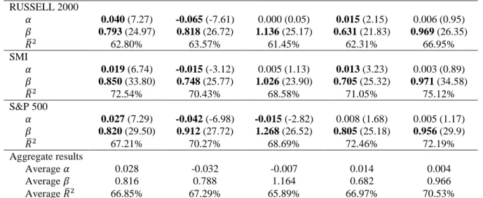
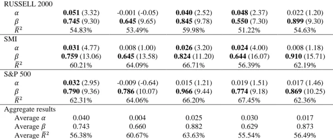
26

Table 3: Univariate regressions for volatility forecasts: 22-day forecast horizon

This table presents results from estimating regressions of realized volatility on individual volatility forecasts. The forecast horizon is 22 trading days. Each panel corresponds to a different market. Columns show estimation results for a particular forecasting model. α and β denote the intercept and slope of the regression, while the row “𝑅̅2_”

shows the adjusted R2 _{coefficient of the regression. Numbers in parentheses denote t-statistics. The bottom panel}

of the table contains the average values of the intercepts and slopes across markets for each forecasting model. All regressions are estimated using Newey-West (1987) heteroskedasticity and autocorrelation consistent standard errors. Forecasts are based on: the lagged realized volatility (LRE), the model-free implied volatility (MFIV), the MFIV adjusted for the volatility risk premium (C-MFIV), the GJR-GARCH(1,1) model (GJR), and, the Heterogeneous Autoregressive (HAR) model. Significant coefficients at the 5% level are highlighted in bold. HAR and GJR model forecasts are produced using a rolling sample of 800 daily observations.

LRE MFIV C-MFIV GJR HAR

AEX 𝛼 0.037 (4.94) 0.011 (1.37) 0.032 (4.51) 0.037 (5.82) 0.010 (1.11) 𝛽 0.743 (13.38) 0.602 (15.08) 0.819 (14.92) 0.580 (17.23) 0.916 (14.49) 𝑅̅2 60.29% 63.05% 67.40% 60.46% 60.32% CAC 40 𝛼 0.039 (4.83) -0.004 (-0.49) 0.026 (3.25) 0.029 (4.02) 0.015 (1.79) 𝛽 0.758 (13.56) 0.743 (15.93) 0.883 (14.55) 0.660 (16.95) 0.898 (15.82) 𝑅̅2 59.10% 62.16% 65.36% 58.30% 59.32% DAX 𝛼 0.046 (4.91) -0.001 (-0.11) 0.028 (2.96) 0.020 (1.79) 0.018 (1.85) 𝛽 0.731 (12.58) 0.745 (14.78) 0.874 (13.64) 0.758 (12.44) 0.877 (14.56) 𝑅̅2 57.07% 63.04% 63.06% 57.04% 55.84% DJIA 𝛼 0.032 (2.79) -0.010 (-0.66) 0.015 (1.11) 0.012 (0.87) 0.024 (2.05) 𝛽 0.783 (8.41) 0.853 (8.95) 0.964 (8.49) 0.856 (8.42) 0.810 (9.01) 𝑅̅2 61.25% 63.75% 66.18% 65.81% 60.23% EURO STOXX 50 𝛼 0.052 (5.41) 0.003 (0.26) 0.026 (2.38) 0.034 (3.65) 0.018 (1.78) 𝛽 0.706 (11.63) 0.724 (12.61) 0.902 (11.69) 0.694 (13.54) 0.896 (14.49) 𝑅̅2 51.97% 59.20% 60.61% 57.86% 51.66% FTSE 100 𝛼 0.025 (3.85) 0.000 (0.05) 0.021 (3.17) 0.024 (3.29) 0.007 (1.02) 𝛽 0.802 (13.26) 0.628 (15.86) 0.863 (13.49) 0.593 (13.01) 0.913 (14.46) 𝑅̅2 64.42% 68.52% 71.44% 62.02% 63.13% HANG SENG 𝛼 0.041 (3.20) 0.026 (3.21) 0.020 (2.42) 0.094 (11.21) 0.022 (1.89) 𝛽 0.701 (6.50) 0.476 (10.59) 0.877 (10.89) 0.180 (5.89) 0.806 (8.35) 𝑅̅2 48.81% 56.42% 57.94% 28.44% 49.71% KOSPI 𝛼 0.049 (3.30) 0.006 (0.30) 0.020 (1.15) 0.002 (0.09) 0.025 (1.27) 𝛽 0.696 (6.29) 0.618 (6.81) 0.916 (6.99) 0.742 (6.39) 0.830 (6.27) 𝑅̅2 48.02% 57.96% 58.81% 46.78% 48.50% NIKKEI 225 𝛼 0.047 (3.44) 0.031 (2.01) 0.033 (2.42) 0.035 (2.47) 0.019 (1.09) 𝛽 0.677 (6.43) 0.456 (6.87) 0.810 (7.58) 0.491 (7.36) 0.841 (6.84) 𝑅̅2 45.67% 49.89% 57.50% 47.43% 46.16% NASDAQ 𝛼 0.033 (3.29) -0.011 (-0.87) 0.019 (1.74) 0.010 (0.85) 0.015 (1.34) 𝛽 0.770 (9.55) 0.662 (10.91) 0.927 (10.35) 0.655 (10.12) 0.889 (10.43) 𝑅̅2 59.04% 63.08% 65.95% 62.84% 60.29%

27

Table 3 continued

LRE MFIV C-MFIV GJR HAR

RUSSELL 2000 𝛼 0.051 (3.32) -0.001 (-0.05) 0.040 (2.52) 0.048 (2.37) 0.022 (1.20) 𝛽 0.745 (9.30) 0.645 (9.65) 0.845 (9.78) 0.550 (7.30) 0.899 (9.30) 𝑅̅2 _{54.83% 53.49% 59.98% 51.22% 54.63%} SMI 𝛼 0.031 (4.77) 0.008 (1.00) 0.026 (3.20) 0.024 (4.00) 0.008 (1.18) 𝛽 0.759 (13.06) 0.645 (13.58) 0.824 (11.20) 0.644 (16.07) 0.910 (15.71) 𝑅̅2 _{60.21% 64.09% 66.71% 56.39% 62.19%} S&P 500 𝛼 0.032 (2.95) -0.009 (-0.64) 0.015 (1.21) 0.019 (1.51) 0.017 (1.46) 𝛽 0.790 (9.36) 0.786 (10.07) 0.966 (9.44) 0.774 (9.18) 0.869 (10.25) 𝑅̅2 _{62.31% 64.06% 66.20% 67.45% 62.36%} Aggregate results Average 𝛼 0.040 0.004 0.025 0.030 0.017 Average 𝛽 0.743 0.660 0.882 0.629 0.873 Average 𝑅̅2 _{56.38% 60.67% 63.63% 55.54% 56.49%}

28

Table 4: Aggregate results from encompassing regressions for the 1-day and 5-day forecast horizons

This table presents average coefficient estimates as well as average adjusted R2 _{coefficients (𝑅̅}2_{) from regressions of realized volatility on competing volatility forecasts at the}

1-day and 5-day forecast horizons, respectively. Each column reports results for a different pair of forecasting models. For example, the column headed “HAR+GJR” contains the aggregate results from estimating a two-variable regression of realized volatility on the forecasts from the HAR and the GJR model, respectively. Forecasting is based on: the lagged realized volatility from 5-minute returns (LRE), the model-free implied volatility (MFIV), the MFIV adjusted for the volatility risk premium (C-MFIV), the GJR-GARCH(1,1) model (GJR), and the Heterogeneous Autoregressive (HAR) model. All regressions are estimated using Newey-West (1987) heteroskedasticity and autocorrelation corrected standard errors.

LRE+GJR LRE+MFIV LRE+C-MFIV HAR+GJR HAR+MFIV HAR+C-MFIV GJR+MFIV GJR+C-MFIV

Panel A: 1-day forecast horizon

Average 𝛼 0.010 -0.016 -0.002 0.000 -0.017 -0.006 -0.017 -0.006

Average 𝛽1 0.429 0.432 0.461 0.613 0.623 0.670 0.375 0.414

Average 𝛽2 0.388 0.439 0.613 0.297 0.316 0.407 0.399 0.555

A