Massachusetts Institute of Technology
Department of Economics
Working Paper Series
The miracle of microfinance?
Evidence from a randomized evaluation
Abhijit Banerjee
Esther Duflo
Rachel Glennester
Cynthia Kinnan
Working Paper 13-09
April 10, 2013
Room E52-251
50 Memorial Drive
Cambridge, MA 02142
This paper can be downloaded without charge from the
Social Science Research Network Paper Collection at
The miracle of microfinance? Evidence from a randomized evaluation
∗ Abhijit Banerjee† Esther Duflo‡ Rachel Glennerster§ Cynthia Kinnan¶This version: April, 2013
Abstract
This paper reports on the first randomized evaluation of the impact of introducing the standard microcredit group-based lending product in a new market. In 2005, half of 104 slums in Hyderabad, India were randomly selected for opening of a branch of a particular microfinance institution (Span-dana) while the remainder were not, although other MFIs were free to enter those slums. Fifteen to 18 months after Spandana began lending in treated areas, households were 8.8 percentage points more likely to have a microcredit loan. They were no more likely to start any new business, although they were more likely to start several at once, and they invested more in their existing businesses. There was no effect on average monthly expenditure per capita. Expenditure on durable goods increased in treated areas, while expenditures on “temptation goods” declined. Three to four years after the initial expansion (after many of the control slums had started getting credit from Spandana and other MFIs ), the probability of borrowing from an MFI in treatment and comparison slums was the same, but on average households in treatment slums had been borrowing for longer and in larger amounts. Consumption was still no different in treatment areas, and the average business was still no more profitable, although we find an increase in profits at the top end. We found no changes in any of the development outcomes that are often believed to be affected by microfinance, including health, education, and women’s empowerment. The results of this study are largely consistent with those of four other evaluations of similar programs in different contexts. JEL codes: O16, G21, D21
∗
This paper updates and supersedes the 2010 version, which reported results using one wave of endline surveys. The au-thors wish to extend thanks to Spandana, especially Padmaja Reddy whose commitment to understanding the impact of mi-crofinance made this project possible, and to numerous seminar audiences and colleagues for insightful suggestions. The Cen-tre for Micro Finance at IFMR oversaw the experiment and the data collection. Aparna Dasika and Angela Ambroz provided excellent assistance in Hyderabad. Justin Oliver at the Centre for Micro Finance and Annie Duflo at Initiatives for Poverty Action shared valuable advice and logistical support. Adie Angrist, Leonardo Elias, Shehla Imran, Seema Kacker, Tracy Li, Aditi Nagaraj and Cecilia Peluffo provided excellent research assistance. ICICI provided financial support. Datasets for both waves of data used in this paper are available at http://www.centre-for-microfinance.org/publications/data/.
†
MIT Department of Economics and NBER. Email: [email protected] ‡
MIT Department of Economics and NBER. Email: [email protected] §
Abdul Latif Jameel Poverty Action Lab and MIT Department of Economics. Email: [email protected] ¶
1
Introduction
Microfinance institutions (MFIs) have expanded rapidly over the last 10 to 15 years: according
to the Microcredit Summit Campaign (2012), the number of very poor families with a microloan
has grown more than 18-fold from 7.6 million in 1997 to 137.5 million in 2010.
Microcredit has generated considerable enthusiasm and hope for fast poverty alleviation. In
2006, Mohammad Yunus and the Grameen Bank were awarded the Nobel Prize for Peace, for
their contribution to the reduction in world poverty. In 2009, the Consultative Group to Assist
the Poor (CGAP), an international organization housed at the World Bank and dedicated to
accelerating financial inclusion, cited the following as contributions of microfinance for which
there was already evidence: eradication of poverty and hunger, universal primary education,
the promotion of gender equality and empowerment of women, reduction in child mortality, and
improvement in maternal health. CGAP was far from alone in its enthusiasm.
The possibility of a “win-win” opportunity, in which the poor could be given the means to
pull themselves out of poverty and microfinance organizations could make a profit (potentially a
big one, as the successful IPO of Compartamos in Mexico, or SKS in India, have demonstrated)
exerts a powerful attraction on policymakers, funding agencies, and academics alike. In the last
several years, however, the enthusiasm for microcredit has been matched by an equally strong
backlash . For instance, a November 2010 article inThe New York Times, appearing in the wake
of a rash of reported suicides linked to MFI over-indebtedness, quotes Reddy Subrahmanyam,
an official in Andhra Pradesh, accusing MFIs of making “hyperprofits off the poor.” He argues
that “the industry [has] become no better than the widely despised village loan sharks it was
intended to replace.... The money lender lives in the community. At least you can burn down
his house. With these companies, it is loot and scoot” (Polgreen and Bajaj 2010). MFIs have
come under attack in India (in Andhra Pradesh, an ordinance making it difficult for them to
operate has pushed several to the brink of bankruptcy), in Latin America (with the “No Pago”
movement), and even in Bangladesh (with a standoff between Yunus and the government over
the leadership of the Grameen Bank). Not unlike credit cards companies or payday lenders in
the US, MFIs are now accused of pushing their clients into debt traps. The stellar repayment
unscrupulous methods.
What is striking about this debate is the relative paucity of evidence to inform it. Anecdotes
about highly successful entrepreneurs or deeply indebted borrowers tell us nothing about the
effect of microfinance on the average borrower, much less the effect of having access to it on the
average household. Even representative data about microfinance clients and non-clients cannot
identify the causal effect of microfinance access, because clients are self-selected and therefore
not comparable to non-clients. Microfinance organizations also purposely choose some villages
and not others. . Difference-in-difference estimates can control for fixed differences between
clients and non-clients, but it is likely that people who choose to join MFIs would be on different
trajectories even absent microfinance. This invalidates comparisons over time between clients
and non-clients (see Alexander-Tedeschi and Karlan 2007).
These issues make the evaluation of microcredit particularly difficult, and there is so far
no consensus among academics on its impact. For example, Pitt and Khandker (1998) use the
eligibility threshold for getting a loan from Grameen bank as a source of identifying variation
in a structural model of the impact of microcredit, and find large positive effects, especially for
women. However, Jonathan Morduch (1998), and Roodman and Morduch (2010) criticize the
approach, pointing out among other issues that there is in fact no discontinuity in the probability
to borrow at that threshold.1
As early as 1999, Morduch wrote that “the ‘win-win’ rhetoric promising poverty alleviation
with profits has moved far ahead of the evidence, and even the most fundamental claims remain
unsubstantiated.” In 2005, Beatriz Armendáriz and Morduch reiterated the same uncertainty in
their book The Economics of Microfinance, noting that the relatively few carefully conducted
longitudinal or cross-sectional impact studies yielded conclusions much more measured than
MFIs’ anecdotes would suggest, reflecting the difficulty of distinguishing the causal effect of
microcredit from selection effects. These cautions were repeated in the book’s second edition in
2010 .
Given the complexity of this identification problem, the ideal experiment to estimate the effect
1Kaboski and Townsend (2005) use a natural experiment (the introduction of a village fund whose size is fixed by village) to estimate the impact of the amount borrowed and find impacts on consumption, but not investment. This is a government-provided form of credit and differs in a number of ways from the standard microcredit product.
of having access to microcredit is to randomly assign microcredit to some areas, and not others,
and compare outcomes in both. Randomization ensures that, on average, the only difference
between residents is the greater ease of access to microcredit of those in the treatment area.2 In this paper we report on the first randomized evaluation of the effect of the canonical
group-lending microcredit model, which targets women who may not necessarily be entrepreneurs.3 This study also follows the households over the longest period of any study (it followed households
for about three to 3.5 years after the introduction of the program in their slums areas), which is
necessary since many impacts may be only expected to surface over the medium run. A number
of recent papers have reported on subsequent randomized evaluations of similar programs in
Morocco (Crépon et al., 2011), Bosnia-Herzegovina (Augsburg et al., 2012), Mexico (Angelucci
et al., 2012) and Mongolia (Attanasio et al. 2011). We will compare their results to ours in the
last section of this paper.4
The experiment was conducted as follows. In 2005, 52 of 104 poor neighborhoods in
Hy-derabad were randomly selected for opening of an MFI branch by one of the fastest-growing
MFIs in the area, Spandana, while the remainder were not. Hyderabad is the fifth largest city in
India, and the capital of Andhra Pradesh, the Indian state were microcredit has expanded the
fastest. Fifteen to 18 months after the introduction of microfinance in each area, a
comprehen-sive household survey was conducted in an average of 65 households in each neighborhood, for a
total of about 6,850 households. In the meantime, other MFIs had also started their operations
in both treatment and comparison households, but the probability of receiving an MFI loans
was still 8.8 percentage points (48%) higher in treatment areas than in comparison areas (27.1%
borrowers in treated areas versus 18.3% borrowers in comparison areas). Two years after this
first endline survey, we surveyed the same households once more. By that time, both Spandana
and other organizations had started lending in the treatment and control groups, so the fraction
of households borrowing from microcredit organizations was not significantly different (38.5% in
2An alternative to measure the impact of borrowing is to randomize microcredit offer among applicants. This approach was pioneered by Karlan and Zinman (2009), which uses individual randomization of the “marginal” clients in a credit scoring model to evaluate the impact of consumer lending in South Africa, and find that access to microcredit increases the probability of employment. Karlan and Zinman (2011) use the same approach to measure impact of microcredit among small businesses in Manila.
3
The two studies mentioned in Footnote 2 evaluate slightly different programs: consumer lending in the case of Karlan and Zinman (2009), and “second generation” individual liability loans to existing entrepreneurs in the case of Karlan and Zinman (2010).
4
treatment and 33% in control). But households in treatment groups had larger loans and had
been borrowing for a longer time period. This second survey thus gives us an opportunity to
examine some of the longer-term impacts of microcredit access on households and businesses.
To frame the analysis, we propose a model where a household may wish to acquire lumpy
investment (a durable good, or an asset for a business ). One key result of the model is that
households who have access to microcredit may sacrifice short- or even medium-term consumption
when microcredit becomes available in order to get the durable good, or to invest in a business.
Other households may decide to expand their labor supply. Non-durable consumption may
thus initially fall, and even total consumption may not increase. Of course, if the household
has invested in a profitable business, we could eventually expect consumption to increase: this
underscores the importance of following households over a long enough period of time.
We examine the effect consumption, new business creation, business income, etc., as well
as measures of other human development outcomes such as education, health and women’s
empowerment. At the first endline, we see no difference in monthly per capita consumption and
monthly non-durable consumption. We do see significant positive impacts on the purchase of
durables. There is evidence that this is financed partly by an increase in labor supply and partly
by cutting unnecessary consumption: households have reduced expenditures on what that they
themselves describe as “temptation goods.”
Thus, in our context, microfinance plays a role in helping households make different
intertem-poral choices in consumption. This is not the only impact that is traditionally expected from
microfinance, however. The primary engine of growth that it is supposed to fuel is business
creation. Fifteen to 18 months after gaining access, households are no more likely to be
en-trepreneurs (that is, have at least one business), but they are more likely to start more than one
business, and they invest more in the businesses they do have (or the ones they start). There is
an increase in the average profits of the businesses that were already in existence before
micro-credit, but this is entirely due to very large increases in the upper tail. At every quantile between
the 5th and the 95th percentile, there is no difference in the profits of the businesses. The
me-dian marginal new business is both less profitable and less likely to have even one employee in
treatment than in control areas.
treatment group households have had the opportunity to borrow for a longer time, businesses
in the treatment groups have significantly more assets, and business profits are now larger for
businesses above the 85th percentile. However, the average business is still small and not very
profitable. In other words, contrary to most people’s belief, to the extent microcredit helps
businesses, it may help the larger businesses more. There is still no difference in average
con-sumption.
We do not find any effect on any of the women’s empowerment or human development
outcomes either after 18 or 36 months. Furthermore, almost 70% of eligible households do not
have an MFI loan, preferring instead to borrow from other sources, if they borrow (and most
do).
Our results find a strong echo in the four other studies that look at similar programs in
different contexts. This gives us confidence in the robustness and external validity of our findings.
In short, microcredit is not for every household, or even most households, and it does not lead
to the miraculous social transformation some proponents have claimed. Its principal impact
seems, perhaps unsurprisingly, to allow some households to sacrifice some instantaneous utility
(temptation goods or leisure) to finance lumpy purchases, either for their home or in order to
establish or expand a business.
2
Experimental Design and Background
2.1 The Product
Until the major crisis in Indian microfinance in 2010, Spandana was one of the largest and fastest
growing microfinance organizations in India, with 1.2 million active borrowers in March 2008, up
from 520 borrowers in 1998-9, its first year of operation (MIX Market, 2009). From its birthplace
in Guntur, a dynamic city in Andhra Pradesh, it has expanded across the state and into several
others.
The basic Spandana product is the canonical group loan product, first introduced by the
Grameen Bank. A group is comprised of six to ten women, and 25-45 groups form a “center.”
Women are jointly responsible for the loans of their group. The first loan is Rs. 10,000, about $200
rates (World Bank, 2007).5 It takes 50 weeks to reimburse principal and interest rate; the interest rate is 12% (non-declining balance; equivalent to a 24% APR). If all members of a group repay
their loans, they are eligible for second loans of Rs. 10,000-12,000; loan amounts increase up to
Rs. 20,000.
Unlike other microfinance organizations, Spandana does not require its clients to start a
business (or pretend to) in order to borrow: the organization recognizes that money is fungible,
and clients are left entirely free to choose the best use of the money, as long as they repay
their loan. Also unlike other microlenders, most notably Grameen, Spandana does not insist on
“transformation” in the household. Spandana is primarily a lending organization, not directly
involved in business training, financial literacy promotion, etc.
Eligibility is determined using the following criteria: clients must (a) be female,6 (b) be aged 18 to 59, (c) have resided in the same area for at least one year, (d) have valid identification
and residential proof (ration card, voter card, or electricity bill), and (e) at least 80% of women
in a group must own their home. Groups are formed by women themselves, not by Spandana.
Spandana does not determine loan eligibility by the expected productivity of the investment,
although selection into groups may screen out women who cannot convince fellow group-members
that they are likely to repay.
2.2 Experimental Design
Spandana initially selected 120 areas (identifiable neighborhoods, or bastis) in Hyderabad as
places in which they were interested in opening branches. These areas were selected based on
having no preexisting microfinance presence, and having residents who were desirable potential
borrowers: poor, but not “the poorest of the poor.” Areas with high concentrations of
con-struction workers were avoided because they move frequently which makes them undesirable as
microfinance clients. While the selected areas are commonly referred to as “slums,” these are
permanent settlements with concrete houses and some public amenities (electricity, water, etc.).
5
In 2007 the PPP exchange rate was $1=Rs. 9.2, while the market exchange rate was $1'Rs. 50. All following references to dollar amounts are in PPP terms unless noted otherwise.
6
Spandana also offers an individual-liability loan. Men are also eligible for individual-liability loans, and individual borrowers must document a monthly source of income, but the other criteria are the same as for joint-liability loans. 96.5% of Spandana borrowers were female in 2008 (Mix Market, 2009). Spandana introduced the individual-liability loan in 2007; very few borrowers in our sample have individual-liability loans.
Within eligible neighborhoods, the largest ones were not selected for the study, since Spandana
was keen to start operations there. The population in the neighborhoods selected for the study
ranges from 46 to 555 households.
In each area, we conducted a small baseline neighborhood survey in 2005, collecting
informa-tion on household composiinforma-tion, educainforma-tion, employment, asset ownership, expenditure, borrowing,
saving, and any businesses currently operated by the household or stopped within the last year.
We surveyed a total of 2,800 households in order to obtain a rapid assessment of the baseline
conditions of the neighborhoods. However, since there was no existing census, and the baseline
survey had to be conducted very rapidly to gather some information necessary for
stratifica-tion before Spandana began their operastratifica-tions, the households were not selected randomly from a
household list: instead field officers were asked to map the area and select every nth house, with
nchosen to select 20 household per area. But this procedure was not very rigorous, and we are not confident that the baseline is representative. Thus, the baseline survey was used as a basis
for stratification, a descriptive analysis below, and area-level characteristics are used as control
variables.7 Beyond this, we do not use the baseline survey in the analysis that follows.
After the baseline survey, but prior to randomization, sixteen areas were dropped from the
study because they were found to contain large numbers of migrant-worker households. Spandana
(like other MFIs) has a rule that loans should only be made to households who have lived in the
same community for at least one year because the organization believes that dynamic incentives
(the promise of more credit in the future) are more important in motivating repayment for these
households. The remaining 104 areas were grouped into pairs of similar neighborhoods, based
on average per capita consumption and per-household debt, and one of each pair was randomly
assigned to the treatment group.8
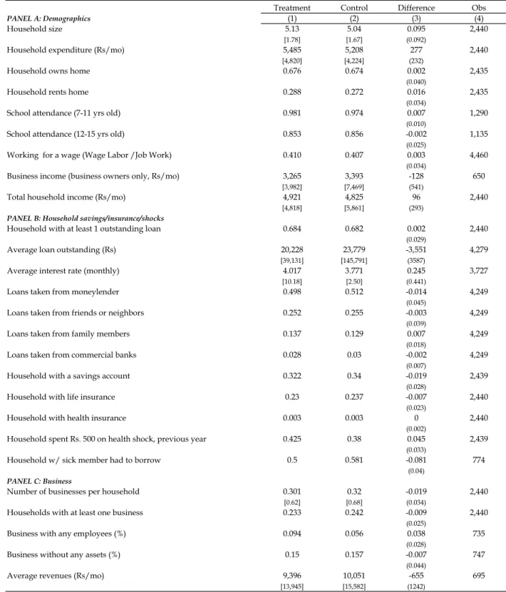
Table 1 uses the baseline sample to show that treatment and comparison areas did not
differ in their baseline levels of demographic, financial, or entrepreneurship characteristics in the
baseline survey. This is not surprising, since the sample was stratified according to per capita
consumption, fraction of households with debt, and fraction of households who had a business.9 7Omitting these controls does not affect the results.
8
Pairs were formed to minimize the sum across pairs A, B (area A avg loan balance – area B avg loan balance)2 + (area A per capita consumption – area B per capita consumption)2. Within each pair one neighborhood was
randomly allocated into treatment.
The baseline data also provides a snapshot of households’ characteristics prior to Spandana’s
expansion, which we discuss further below.
Spandana then progressively began operating in the 52 treatment areas, between 2006 and
2007. Note that in the intervening periods, other MFIs also started their operations, both in
treatment and comparison areas, and we did nothing to stop that. We will show below that there
is still a significant difference between MFI borrowing in treatment and comparison groups.
To create a proper sampling frame for the endline, we undertook a comprehensive census of
each area in early 2007, and included a question on borrowing. The census revealed low rates
of MFI borrowing even in treatment areas, so the endline sample consisted of households whose
characteristics suggested high likelihood of having borrowed: households who had resided in
the area for at least three years and contained at least one woman aged 18 to 55. Spandana
borrowers identified in the census were oversampled, and the results presented below correct for
this oversampling so that the results are representative of the population as a whole. Since they
were not representative, baseline households were not purposely resurveyed in the follow-up.
We began the endline survey in August 2007 and ended it in April 2008. In each area, this
first endline survey was conducted at least 12 months after Spandana began disbursing loans,
and generally 15 to 18 months after. The overall sample size for the endline survey was 6,864
households.
Two years later, in 2009-2010, we undertook a second endline survey, following up on the same
households, asking the same set of questions as in 2007-2008 to insure comparability. Appendix
Table 2, Panel A shows, the re-contact rate at endline 2 for household initially interviewed at
endline 1 was very high, at 89.9% in the treatment group and 90.2% in the control group. Panel
B shows average characteristics of the recontacted versus attrited households. The samples do
not differ significantly along most dimensions. However, those who attrited had higher per capita
expenditure at endline 1, by Rs. 131 (column 1). Attritors were five percentage points less likely
to have an MFI loan at endline 1 (column 5), and 1.5 percentage points less likely to have a
business created in the one year prior to endline 1 (column 7). This is consistent with businesses
and microloans being associated with lower mobility, and higher consumption/permanent income
endline are similar in treatment and control groups, in terms of a number of characteristics which are fixed over time (Table A1).
being associated with higher mobility. Panel C shows that one important characteristic
differen-tially predicts attrition in treatment versus control, namely MFI borrowing: the attrited sample
is nine percentage points less likely than the non-attrited sample to have had an MFI loan in
treatment areas. This suggests that Spandana was effective in either targeting households that
were going to stay put, or convincing them not to leave the area.10
2.3 The context
Table 1 shows a snapshot of households from the 104 sampled areas in 2005. Recall that these
numbers need to be viewed with some caution, as the households sampled at baseline were not
necessarily representative of the area as a whole, and were not purposely resurveyed at endline.
At baseline, the average household (averaging over treatment and control areas) was a family of
five, with monthly expenditure of just under Rs. 5350, or $540 at PPP-adjusted exchange rates
($108 per capita) (World Bank, 2005). A majority of households (67%) lived in a house they
owned, and 27% in a house they rented.11 Almost all of the 7 to 11 year olds (98%), and 86% of the 12 to 15 year olds, were in school.
There was almost no MFI borrowing in the sample areas at baseline. However, 68% of the
households had at least one outstanding loan. The average amount outstanding was Rs. 21,658
(median Rs. 11,000), and the average interest rate was 3.89% per month. Most loans were taken
from moneylenders (50%), friends or neighbors (25%), and family members (13%). Commercial
bank loans were very rare (3%).
Although business investment was not commonly named as a motive for borrowing, 24% of
households ran at least one small business at the baseline, compared to an OECD-country average
of 12% who say that they are self-employed. However, these businesses were very small. Only
7.5% had any employees; typical assets included sewing machines, tables and chairs, balances and
10
While attrition rates are comparable in treatment and comparison areas, the differential attrition according to propensity to borrow from an MFI is potentially concerning, not only for the analysis of endline 2 data, but possibly for endine 1 as well: endline 1 data may suffer from attrition, although we do not observe it since we do not have a baseline. To address this concern, we have re-estimated all the regressions below with a correction for sample selection inspired by Dinardo, Fortin and Lemieux (2010), where we re-weight the data using the inverse of the propensity to be observed at endline 2, so that the distribution of observable characteristics (at endline 1) among households observed at endline 2 resembles that in the entire endline 1 sample. We then apply the same weights to endline 1 data (implicitly assuming a similar selection process between the onset of microfinance and endline 1). The results, available upon request, are very similar to what we present here.
11
pushcarts, and 15% of businesses had no assets whatsoever. Average revenues were approximately
Rs. 9,900 ($980 in PPP terms) per month on average. Business income (i.e., profits) were
approximately Rs. 3,300 ($325 at PPP). Total household income, from entrepreneurship, wage
labor, irregular labor, etc. averaged approximately Rs. 4,840. Forty-two percent of working
individuals worked for a wage.
Baseline data revealed more limited use of consumption smoothing strategies other than
borrowing: 34% of the households had a savings account, and only 23% had a life insurance
policy. Almost none (0.03%) had any health insurance. Forty percent of households reported
spending Rs. 550 ($54) or more on a health shock in the last year; 50% of households who had
a sick member had to borrow for a health-related purpose.
Growth between 2005 and 2010
Table 2, shows some of the same key statistics for the endline 1 and endline 2 (EL1 and EL2)
samples in the control group.
Comparing the control baseline sample (2005) with the control households in the EL1 (2008)
and EL2 (2010) samples reveal rapid secular growth in Hyderabad over 2005-2010.12 Average household consumption rose from Rs. 5,485 to Rs. 7,662 in 2007 and Rs. 11,497 (all expressed
in 2007 rupees). in EL2. There was a 12 percentage point increase in the likelihood the family’s
house was waterproof between baseline and EL2 (68% versus 56%). Eighty-one percent of families
owned a color TV at EL2, up 20 percentage points from two years before and 50 percentage points
from the baseline. The fraction owning a cellphone increased from 17% at baseline to 64% at
EL1 and 86% at EL2.
The percentage of households who ran at least one small business increased from 24% at
baseline to 34% at EL1 and 42% at EL2. Forty-three percent of these businesses were primarily
operated by a woman. However, the businesses remain very small: only 9% (10%) had any
employees at EL1 (EL2). Yet despite remaining very small in terms of employment, average
revenues rose from approximately Rs. 9,900 ($980 in PPP terms) per month on average at
baseline to just over Rs. 11,000 at EL1 and almost 16,000 at EL2. At EL2, business owners
12
While the comparison may not be perfect since the baseline survey was not conducted on the same sample as the endline, the growth between EL1 and EL2 is for the same set of households, using the same survey instruments, and thus gives us a good sense of the dynamism of this economy.
reported business income (profits) of almost Rs. 5,000 (~$540 at PPP), up from about Rs. 2,500
($275) at EL1. (These profit estimates do not account for the cost of the proprietors’ time.)
The fraction of households with at least one outstanding loan rose from 68% at baseline to
89% in EL1 and 90% in EL2. The use of consumption-smoothing strategies other than borrowing
also increased. From 34%, the fraction of households with a savings account skyrocketed to 82%
at EL1 and 85% at EL2, and the fraction with health insurance rose from almost 0 at baseline
to 12% at EL1 and 76% at EL2, likely due to the expansion of the government’s RSBY health
insurance program from those below the poverty line. Nonetheless, at EL1 (EL2), 64% (78%) of
households reported spending Rs. 500 or more on a health shock in the last year. The fraction
of households who had a sick member that had to borrow held fairly constant: 50% at baseline
to 53% at EL1 and 45% at EL2.
2.4 Treatment impact on MFI borrowing and borrowing from other sources
Treatment communities were randomly selected to receive Spandana branches, but other MFIs
also started operating both in treatment and comparison areas. We are interested in testing
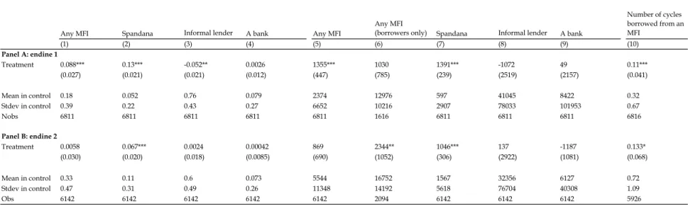
the impact of microcredit, not only borrowing from Spandana. Table 3 Panel A shows that,
by the first endline, MFI borrowing was indeed higher in treatment than in control slums,
al-though borrowing from other MFIs made up for part of the difference in Spandana borrowing.
Households in treatment areas are 13.3 percentage points more likely to report being Spandana
borrowers–18.5% versus 5.2% (Table 3 Panel A, column 2). The difference in the percentage
of households saying that they borrow from any MFI is 8.8 points (Table 3 Panel A, column
1), so some households who ended up borrowing from Spandana in treatment areas would have
borrowed from another MFI in the absence of the intervention. While the absolute level of total
MFI borrowing is not very high, it is about 50% higher in treatment than in comparison areas.
Columns 5 and 7 show that treatment households also report significantly more borrowing from
MFIs (and from Spandana in particular) than comparison households. Averaged over borrowers
and non-borrowers, treatment households report Rs. 1,391 more borrowing from Spandana than
do control households, and Rs. 1,355 more from all MFIs.
While both the absolute take up rate and the implicit “first stage” are relatively small,
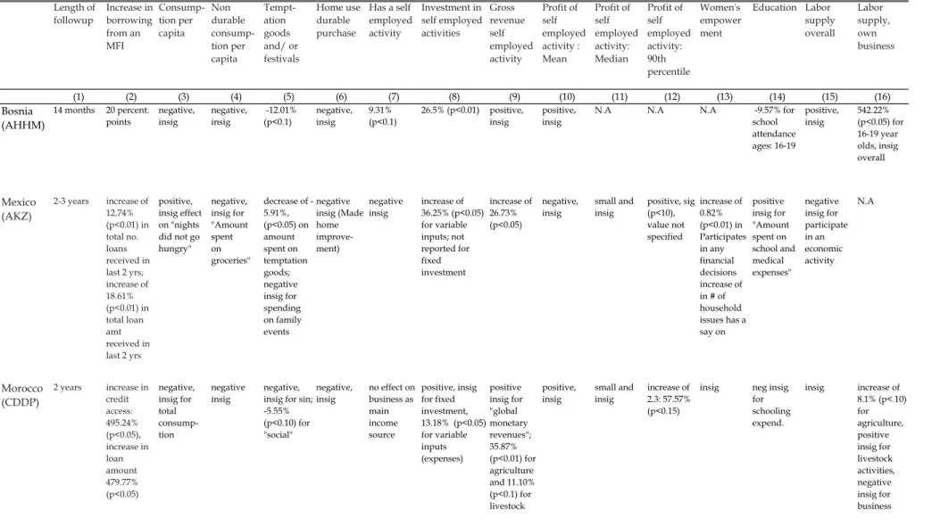
microfinance, despite the different contexts. In rural Morocco, Crépon et al. (2011) find that
the probability of having any loan from the MFI Al Amana in areas which got access to it
is 10 percentage points, whereas it is essentially zero in control, and moreover, since there is
really no other MFI, this represents the total increase in microfinance borrowing. In Mexico,
Angelucci, Karlan and Zinman (2012) find an increase in 10 percentage points in the probability
of borrowing from the MFI Compartamos in areas that got access to the lender, relative to a
base of five percentage points in the control (they don’t report the probability to borrow from
any other MFI). In Mongolia, Attanasio et al. (2011) find a much larger increase, 48 percentage
points, but this is among a sample that had already expressed interest in obtaining a loan from
the lender and formed a potential borrowing group before randomization.13
The fairly low take up rate in these difference contexts is in itself is a perhaps surprising
result, given the high levels of informal borrowing in these communities and the purported
benefits of microcredit over these alternative forms of borrowing. . In all cases, except when the
randomization was among those who had already expressed explicit interest in microcredit, only
a minority of “likely borrowers” end up borrowing.
Table 3 also displays the impact of microfinance access on other forms of borrowing. A
sizable fraction of the clients report repaying a more expensive debt as a reason to borrow from
Spandana, and we do indeed see some action on this margin, but column 3 shows that the share
of households who have some informal borrowing–defined as borrowing from family, friends,
moneylenders and goods purchased on credit–goes down by 5.2 percentage points in treatment
areas, but bank borrowing is unaffected. The point estimate of the amount borrowed from
informal sources is also negative, suggesting substitution of expensive borrowing with cheaper
MFI borrowing (an explicit objective of Spandana), and the point estimate, though insignificant,
is quite similar in absolute value to the increase in MFI borrowing (column 8). However, given the
high level of informal borrowing, this corresponds to a decline of only 2.6%: When we examine
the distribution of endline 1 informal borrowing, in Figure 1, informal borrowing is significantly
lower in treatment areas from the 30th to 65th percentiles.
After the end of the first endline, following our initial agreement with Spandana, the control
13
The last study with which we consider, Augsburg et al. (2012), is not strictly comparable to ours because the sampling frame is made up of people who had applied for a loan. But even there the difference in borrowing rates between treatment and control group is fairly low, only 20 percentage points.
slums were “released,” and Spandana was free to expand in these areas. Other MFIs also
con-tinued their expansion. However, two years later a significant difference still remained between
Spandana slums and others: Table 3 Panel B shows that 18% of the households in the treatment
slums borrowed from Spandana, against 11% in the control slums. Other MFIs continued to
expand both in the former treatment and control slums, and MFI lending overall was almost the
same in the treatment and the control group. By the second endline survey, 33.1% of households
had borrowed from an MFI in the former control slums, and 33.7% in the treatment slums. Since
lending started later in the control group, however, households in the treatment group had on
average been borrowing for longer than those in the control group, which is reflected in the fact
that they had completed more loan cycles. On average, there was a difference of 0.13 loan cycles
between the treatment and the control households at endline 2 (column 10), which is almost
unchanged from endline 1. . The key difference between treatment and control group at endline
2 is thus the length of access to microfinance. Since microfinance loans grow with each cycle,
treatment households also had larger loans. Among those who borrow, there was by the endline
2 a significant difference of Rs. 2,344 (or 14%) in the size of the loans (column 6). Since about
one third of households borrow, this translates into an (insignificant) difference of about Rs. 869
in average borrowing (column 5).
3
Theory
Since the stated goal of many MFIs is to help their client escape poverty by investing in their own
businesses, evaluations of microfinance programs (including this one) typically focus on business
investments and overall consumption per capita as key measures of success. However, to the
extent that microfinance successfully relaxes credit constraints, we may see households sacrifice
short-run non-durable consumption to invest in durable goods (either for home consumption or
for their businesses). The short-run impact (as people take the loan and then repay it) may
therefore be to reduce non-durable consumption or even overall consumption. The increase
in welfare would either come from the utility arising from the durable consumption or, in the
longer run, if the investment makes the borrower’s businesses more profitable and that feeds into
need to pay attention to its composition. Also, a relatively long horizon may be necessary to
determine the full effects. The simple model below clarifies this intuition in order to provide a
conceptual frame to our analysis.
3.1 Basic Model
A consumer lives forT 2periods. We assume just for expositional convenience thatT is even. She consumes two goods which we will call non-durable and durable. The non-durable is fully
divisible and is consumed in the period it is bought. Denote non-durable consumption by cn.
The durable lasts for two periods, and yields durable services in both periods. The durable is
indivisible and costs an amount cd, and yields durable services ofacd in each period. Moreover
there are no additional benefits from owning a second durable. Assume that durable services and
non-durables are perfect substitutes in the sense that the consumer’s per-period utility function
isu(c),wherec=cn if she has not purchased the durable in the current or previous period and
c = cn+acd otherwise. Assume that 0 < a < 1. Therefore in the current period purchasing
the durable leads to a net loss in flow utility, but it might still be optimal because acould be greater than 1/2.The consumer does not discount and the future and therefore maximizes total of present and future utility.
The consumer earns a labor income ofy in units of the non-durable every period and there is no savings or investment, so the total amount y is spent every period. However, the household has the option of borrowing up to an amount bmax for one period at a gross interest rate r. We assume, in keeping with the microfinance application, that the person cannot borrow again till
after the loan is fully repaid. In other words, if the borrower borrows in period s, she will have to repay in period s+ 1and can only borrow again in period s+ 2.Finally we assume that the durable costs more than the maximum possible amount of debt: cd> bmax
Given this, the consumer’s problem in each period depends just on whether she already owns
the durable and her existing stock of debt. If she owns the durable she has no reason to buy it
in the current period; if she has debt then she has to repay it in the current period and cannot
3.2 Analysis of the model
The structure of this model yields a very useful simplification. In the Theoretical Appendix we
show that the consumer’s decision can be analyzed by simply looking at the decision in the first
two periods, assuming that there are no further periods. The decision in the first period will
be repeated in all subsequent odd periods and what happens in period 2 will be repeated in all
subsequent even periods.
This is very convenient because we can study the decision diagrammatically. In Figure 2, the
horizontal axis represents consumption in period 1 and the vertical axis is consumption in period
2. U U and U0U0 are two potential indifference curves. They both have slope 1/δ when they intersect the 45 degree line, OO0 at points E and E0. The point E represents the endowment, the vector (y, y).The line EF, which has the sloper, represents the set of options open to the consumer if he borrows in period 1 but does not purchase the durable. The distance along the
horizontal direction fromE toF representsbmax,the maximum possible loan size. As drawn, we are assuming thatr <1/δ,which gives the consumer a reason to borrow–the highest indifference curve reachable on EF is typically higher that the one throughE.
The other option is to buy the durable. The point A represents the case of just buying the durable and not borrowing, i.e. it is the point (y−(1−a)cd, y +acd). The line segment AB
represents the set of choices for someone who borrows and buys the durable. The horizontal
distance fromA to B is bmax and the slope of the line isr. As drawn, it is clear that the point
B lies on the highest indifference curve that is available and the consumer will choose both to borrow and to buy the durable. However, her first-period consumption is still lower than at
pointE.Non-durable consumption and even total consumption goes down in the first period as a result of purchasing the durable.
However, this is not the only possibility. The point B0 represents what happens when bmax
is higher (F0 is the corresponding point where the consumer borrows without purchasing the durable). In this case, borrowing and buying the durable is still the best option, but total
consumption goes up in both periods. Finally, the point B00 represents the case where bmax is small. F00 is the corresponding value in the case where there is no durable purchase. In this case, borrowing without buying the durable is the best option, and first-period consumption goes up.
lineEF lies everywhere under the indifference curve throughE. However, borrowing to buy the durable still makes sense and improves welfare.
In general, more credit (weakly) increases the incentive to buy the durable relative to either
not buying but borrowing or not buying and not borrowing. To see this denote the utility of
buying the durable as vd(bmax), and that of not buying the durable by vn(bmax).
d dbmaxvd(b max) =max{ d db[u(y−(1−a)cd+b)+δu(y+cd−rb)],0}=max{u 0(y−(1−a)c d+b)−δru0(y+acd−rb),0}
which, by the concavity of uis always at least as large as dvn(bmax)
dbmax =max{dbd[u(y+b) +δu(y−
rb)],0}=max{u0(y+b)−δru(y−rb),0}.Therefore this is also true at the point wherevd(bmax) =
vn(bmax),which tells us that if is tells us that if at any level of bmax vd(bmax)> vn(bmax),then
this is also true at all higher values ofbmax.In this sense, increased access to credit favors buying the durable.
Moreover, it is evident that when the consumer switches to buying the durable as a result
of increased credit access, his borrowing must go up. Hence, compared to someone who has less
credit access, his second-period non-durable consumption,y−rbmust be lower.
Result 1: Compare two people, one of whom has higher access to credit. She is more likely to
buy the durable, but her first-period total non-durable consumption and even total consumption
may be higher or lower. Her second-period non-durable consumption will be lower.
3.3 Extensions
We have so far ignored possibility of making a productive investment. Note however that the
model where there are no durables but the consumer has a choice of investing a fixed amount
(1−a)cd in period 1 to get a return of acd in period 2 is formally identical to the model
with durables and the same reasoning applies. However, the change in interpretation makes
worth emphasizing that since a higher ameans a more productive project, for a high enough a
the investment will be made even when access to credit is very limited or absent. Conversely,
increased access to credit will encourage consumers with relatively low values of ato invest.
Result 2: Increased access to credit increases the likelihood that the consumer makes a
first-period consumption can go up or down with greater credit access. However, in this case the
person will have higher second-period non-durable consumption, since that is the reason for the
investment.
Next, consider a variant of the model where the consumer also has a labor supply decision.
Assume that the consumer can earn w units of non-durable consumption per unit of labor and suppliesl1 andl2 units of labor in periods 1 and 2. The disutility of labor is given by the function
v(l)which is assumed to be increasing, convex, differentiable everywhere and satisfying the Inada condition atl= 0.The consumer now maximizes
u(y−(1−a)cd+b+wl1)−v(l1) +δ[u(y+cd−rb+wl2)−v(l2)
if she buys the durable and
u(y+b+wl1)−v(l1) +δ[u(y−rb+wl2)−v(l2)]
if not.
By our assumptions about v,an interior optimum forl always exists and is given by
u0(c) =v0(l).
It is evident thatl is decreasing inc.Furthermore, iful(x) =maxl{u(x+wl)−v(l)},it is easy
to show that ul(x) inherits the concavity of u(c) and therefore Result 1 extends to this case.
In other words, improved loan access may lead to a reduction in non-durable and even total
consumption in the first period. If total consumption goes down, labor supply will go up in that
period.
Result 3: Increased access to credit can lead to an increase in labor supply in the first
period.
Finally, the assumption that durables and non-durables are perfect substitutes is convenient
for diagrammatic analysis but not essential for our results. Suppose, on the contrary, durable
consumption of cd leads to an utility equal to the service flow from the durable acd, which is
argument that Result 1 will still hold. The only change is that now labor supply only depends
on non-durable consumption, and since non-durable consumption can be lower in both periods,
labor supply may be permanently raised by improved credit access.14
Result 4: If durables and non-durables are not perfect substitutes, increased access to credit
may raise labor supply in both periods.
3.4 Discussion
The main point made in the theoretical section is that increased access to credit can lead to
lowered non-durable consumption, both when the loan is taken and while it is being repaid,
and increased labor supply, potentially once again both when the loan is taken and while it is
being repaid. Durable consumption must, of course, go up if the point of the borrowing is to
buy a durable (though it may not be picked up depending on when in the borrowing cycle the
comparison is made), but not necessarily if the point is to start a business.
To interpret the results below, we consider that the period between the baseline and endline
1 corresponds to two model periods (one borrowing cycle), and the period between endline 1 and
endline 2 corresponds to the next two model periods (one borrowing cycle). This is realistic,
as the baseline happened roughly 15 to 18 months after Spandana started its operation in each
slum, and the average borrowing household had been borrowing for a quarter.
The model tells us that the second borrowing cycle can be just like the first, if there are
multiple durables to buy. In this case, we may see very little difference between those who got
credit access on the first round with those who got it later, except to the extent that the loan size
goes up from round to round–bigger loans may allow buying bigger durables. Of course, if the
durables actually last for more than two periods, those who have access to microfinance earlier
will have a larger stock of durables. On the other hand, if credit is used in both periods to invest
in a business and those businesses are in fact profitable, consumption should be higher in endline
2 for households in the initial treatment group since they are already enjoying the business
returns, while control households have yet to do so.15 Observing the dynamic of treatment effect 14The same result also holds when instead of durables and non-durables, the consumer chooses between a divisible consumption good and a non-divisible one (say, a wedding).
15This is, of course, unless they borrow more and invest everything in the business, in which case we may see higher profits, but potentially consumption that is no higher.
across two borrowing cycles, with one group gaining access one round later, is therefore useful
in assessing the overall impact of microcredit on poverty.
4
Results
To estimate the impact of microfinance becoming available in an area, we focus on intent to
treat (ITT) estimates; that is, simple comparisons of averages in treatment and comparison
areas, averaged over borrowers and non-borrowers. We present ITT estimates of the effect of
microfinance on businesses operated by the household; and for those who own businesses, we
examine business profits, revenue, business inputs, and the number of workers employed by the
business. (The construction of these variables is described in Appendix 2.) Each column reports
the results of a regression of the form
yia=α+β×T reatia+X
0
aγ+εi
whereyia is an outcome for household iin areaa,T reatia is an indicator for living in a treated
area, and β is the intent to treat effect. Xa0 is a vector of control variables, calculated as area-level baseline values: area population, total businesses, average per capita expenditure, fraction
of household heads who are literate, and fraction of all adults who are literate.16 Standard errors are adjusted for clustering at the area level and all regressions are weighted to correct for
oversampling of Spandana borrowers.
4.1 Consumption
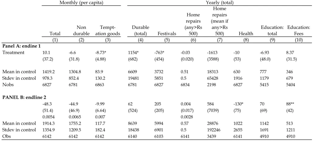
Table 4 gives intent to treat estimates of the effect of microfinance on household spending.
Columns 1 and 2 of Panel A shows that there is no significant difference in total household
expenditures–either total or non-durable–per adult equivalent, between treatment and
compar-ison households. The point estimate is essentially zero in both cases and we can reject the null
hypothesis that there was a Rs. 85 per month increase in consumption per adult equivalent
and Rs. 56 (about 6% of the average in control for consumption, and 4% for non-durable
con-16Table A1 shows that treatment and comparison areas are balanced in terms of these characteristics so, as expected, the results are very similar, although slightly less precise, if these controls are omitted.
sumption) increase. Thus enhanced microcredit access does not appear to be associated with a
significant increase in consumption after 15 to 18 months. Of course, this may partly be due
to the fact that relatively few people borrow, and that some in the control group borrow from
another MFI; still, even if the entire increase (decrease) in total (non-durable) consumption was
due to borrowers, these point estimates thus suggest very modest effects of borrowing.17
While there are no significant impacts on average consumption and non-durable consumption,
there are shifts in the composition of expenditure: column 4 shows that households in treatment
areas spent a statistically significant Rs. 1154 more on durables over the past year than did
households in comparison areas. Note that this is probably an underestimate of the total effect
of loans on durable purchases, since our measure would miss anyone who borrowed more than a
year before the survey (the survey was 15 to 18 months after the centers opened) and immediately
bought a durable with the loan proceeds. The most commonly purchased durables include gold
and silver, motorcycles, sarees (purchased in bulk, presumably mainly for weddings), color TVs,
fridges, rickshaws, computers and cellphones.
Consistent with the model, column 2 shows that while there was no detectable change in
non-durable spending otherwise, the increase in durable spending by treatment households was
essentially offset by reduced spending on “temptation goods” and festivals. Temptation goods
are goods that households in our baseline survey said that they would like spend less on (this
is thus the same list of goods for all households). They include alcohol, tobacco, betel leaves,
gambling, and food consumed outside the home. Spending on temptation goods is reduced by
about Rs. 9 per family per month (column 3). We also see in column 5 a large fall in festival
spending per capita in the previous year (Rs. 763, significant at the 10% level). Together, the
average drop in consumption in temptation goods and festivals over the year is Rs. 1255 per
family and per year, which is reasonably close to the average increase in durables spending of
Rs. 1154 plus the average interest difference of Rs. 325. The remaining difference of about Rs.
225 per family per year is probably matched by extra labor earnings (labor supply increases by
3.23 hours per week).18 The decrease in festival expenditures does not come from large changes 17For total consumption, the implied IV estimate is a Rs. 113 (10/.088) or 5% increase, and for non-durable it is a Rs. 75 (4%) decrease.
18Rs. 1255 comes from 763+8.73*4.68*12 where 8.73 is the reduction on temptation good spending per capita per month and 4.68 is average household size. Rs. 325 comes from 0.24*1355 where 24% is the interest paid on the net extra MFI borrowing of Rs. 1355. Households in the treatment group also spend on average an extra Rs.
in large, very expensive ceremonies such as weddings (we see very few of them in the data) but
rather appears to come from declines at all levels of the distribution of spending on festivals.
This is consistent with the model, assuming that every month (a subperiod of our model), some
households get a chance to make a lumpy expenditure if they can and want to pay for it. We
then see them undertake a large expense (this is more likely in microcredit borrower households
because they have the money). The expense is paid from small, monthly cuts in the non-necessary
non-durable goods (temptation goods and festivals) and spread across both households who have
already made the lumpy purchase and households that anticipate doing so in the future.19 Panel B of Table 4 reports on the impact effects at the time of the second endline, when
both treatment and control households have access to the microfinance program. The effects on
both total per capita spending and total per capita non-durable spending (columns 1 and 2) are
negative with t-statistics around 1. Spending on temptation goods is still lower by about Rs. 10
per month (column 3), similar to endline 1, though the effect is now insignificant. The effect on
festivals is now positive but nowhere near being significant. Overall, the substantial gap between
treatment and control households in terms of avoidable non-durable spending we saw in the first
endline has shrunk to about Rs. 375 per year in endline 2. Correspondingly, there is no difference
on average in durable goods spending in endline 2 (column 4). Given that the main difference
between treatment and control households at endline 2 is that treatment households have been
borrowing for longer, this suggests that, in the second cycle, households in the treatment seem
to just repeat the first cycle with another durable (of roughly the same size), while households
in the control group also acquire a durable.
The absolute magnitude of these changes is relatively small: for instance, the Rs. 1154 of
increased durables spending at endline 1 is approximately $125 at 2007 PPP exchange rates.
However, this represents an increase of about 17% relative to total spending on durable goods in
comparison areas. Furthermore, this figure averages over non-borrowers and borrowers. If all of
this additional spending were coming from the extra 8.8% who do borrow (that is, if there were
no spillover effects to non-borrowers), then the implied increase per additional borrower would
389 per year acquiring business assets compared to households in control group but they also make Rs. 357 more in profits (not significant) which would potentially balance it out.
19Households do not have to spend the loan as soon as they get it. We see examples of households taking a loan and putting it in a savings account for some time before they spend it.
be more than twice the level of durable goods spending in comparison areas. However, since it
is entirely possible that there are spillover or general equilibrium effects (as analyzed by Buera
et al. 2011), and effects that operate through the expectation of being able to borrow when
needed (such as reductions in precautionary savings, as documented in Thailand by Kaboski
and Townsend (2011) and in India by Fulford (2011)), or through general-equilibrium effects on
prices or wages (Giné and Townsend 2004), we will focus here on reduced-form/intent to treat
estimates.
4.2 New businesses and business outcomes
The basic version of our model describes the situation of a household deciding whether to acquire
a durable good. However, as we discuss in the extension (Section 3.3), it can also apply to the
decision to invest in a new or existing business. Most microcredit organizations seek to help
poor women become entrepreneurs or improve the profitability of their business, and it is thus
important to investigate the effect on business creation and expansion.
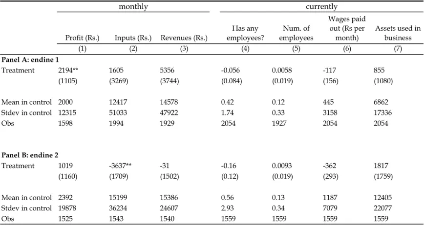
Panel A in Table 5 presents the results from the first endline on business outcomes. Column
1 indicates that the probability that a household starts a business is in fact not significantly
different in treatment and control areas. In comparison areas, 4.7% of households opened at
least one business in the year prior to the survey, compared to 5.6% in treated areas. However,
treatment households weresomewhat more likely to have opened more than one business in the
past year, and column 2 shows that more businesses were created in treatment areas overall:
5.3 per 100 households in control versus 6.9 per 100 households in treatment. The numbers
are small because there are few businesses opened in any given year, but the treatment effect
represents a significant proportional increase (30% more business were created in treatment than
in comparison areas).
Consistent with the fact that Spandana loans only to women, and with the stated goals of
microfinance institutions, the marginal businesses tend to be female-operated: column 3 shows
that when we look at creation of businesses that are owned by women,20 we find that almost all of the differential business creation in treatment areas is in female-operated businesses–there
20
A business is classified as owned by a woman if the first person named in response to the question “Who is the owner of this business?” is female. Only 72 out of 2674 businesses have more than one owner. Classifying a business as owned by a woman if any person named as the owned is female does not change the result.
are 0.015 percentage points more female-owned businesses in treatment than in control areas, an
increase of 58%. Households in treated areas were no more likely to report closing a business,
an event reported by 3.9% of households in treatment areas and 3.7% of the households in
comparison areas (column 4).21
Consistent with the fact that treatment households start more businesses, they invest more in
durables for the business. Since only a third of households have a business, and most businesses
use no asset whatsoever, the point estimate is small in absolute value (Rs. 389 over the last year,
or a bit less than a third of the increase in average MFI borrowing in treatment households) but
the increment in treatment is more than the total value of business durables purchased in the
last year by comparison households (Rs. 280), and is statistically significant.
The rest of the columns in the Panel A of Table 5 report on current business status and
last month’s revenues, inputs costs, and profits. In these regressions, we assign a zero to those
households who do not have a business, so these results give us the overall impact of credit
on business activities, including both the extensive and intensive margins. Consistent with the
prior results, treatment households are no more likely to have a business (summing over those
created in the last year and those created before) but they have more business assets (although
the t-statistic on the asset stock is only 1.58). The treatment effects on revenues and inputs are
both positive but insignificant.
Finally, there is an insignificant increase in business profits. Since this data includes zeros for
households who do not have a business, this answers the question of whether microcredit, as it
is often believed, increases poor households’ income by expanding their business opportunities.
The point estimate, at Rs. 357 per month corresponds to a roughly 50% increase relative to the
profits received by the average comparison household. This is thus large in proportion of profits,
but it represents only a very small increase in disposable income for an average households–recall
that the average total consumption of these households is about Rs. 7,000 per month and an
increase of Rs. 357 per month in business revenues is certainly not going to change the life of
the average person who gets access to microcredit.
That does not rule out that the businesses of some specific groups could have benefit from
21
It is possible that households not represented in our sample, such as households who had not lived in the area for three years, may have been differentially likely to close businesses in treated areas. However, the relatively small amount of new business creation makes general-equilibrium effects on existing businesses rather unlikely.
the loan. To look at this in more detail, we focus on businesses that were already in existence
before microcredit started. We do this in Table 6.22 For businesses that existed before Spandana expanded, we find an average increase in profits of Rs. 2194 in treatment areas, which is
signif-icant and more than double the control mean. This increase, however, is entirely concentrated
in the upper tail (quantiles 95 and above), as shown in Figure 4. At every other quantile, there
is very little difference between the profits of existing businesses in treatment and control areas.
The 95th percentile of monthly profit of existing businesses is Rs. 14600 (or $1590 at PPP),
which makes them quite large and profitable businesses in this setting. The vast majority of the
small businesses make very little profits to start with, and microcredit does nothing to help them.
This absence of an effect on the average business is consistent with the results of Karlan and
Zinman (2011), who evaluate individual loans given to micro-entrepreneurs in the Philippines,
and do not find that the loans result in an increase in profits. The finding that microcredit is
most effective in helping larger businesses is contrary both to much of the rhetoric of microcredit
and the view of microcredit skeptics.
Finally, we have seen that the treatment led to some more business creation, particularly
female-owned businesses. In Figure 5, and Tables 7 and A3, we show more data on the
charac-teristics of these new businesses. The quantile regressions in Figure 5 (profits for businesses that
did not exist at baseline) show that all businesses between the 35th and 65th percentiles have
significantly lower profits in treatment areas. Table 7, column 1 shows that the mean profit is
not significantly different across treatment and control due to the noisy data, but the median
new business in treatment areas has Rs. 1250 lower profits, significant at the 5% level (Table
7, column 2). The average new business is also significantly less likely to have employees in the
treatment areas: the proportion of the new businesses that have any employee falls from 9.4%
to only 4.5% (column 5).
These results could in principle be a combination of a treatment effect and a selection effect,
but since the effect on existing businesses suggests a treatment effect which is close to zero
for most businesses (and the point estimate is positive), the effect for new businesses is likely
due to selection–the marginal business that gets started in treatment areas is less profitable
22
In Table 5, we show that households are no more or less likely to close a business in the last year, thus there is no sample selection induced by microfinance.
than the marginal business in the control areas. The hypothesis that the marginal business
which gets started is different in the treatment group gains some additional support in Appendix
Table 3, which shows a comparison of the industries of old businesses and new businesses, across
treatment and comparison areas.23 Industry is a proxy for the average scale and capital intensity of a business, which is likely to be measured with less error than actual scale or asset use. The
industry composition of new businesses do differ. In particular, the fraction of food businesses
(tea/coffee stands, food vendors, kirana stores, and agriculture) is 8.5 percentage points (about
45%) higher among new businesses in treatment areas than among new businesses in comparison
areas, and the fraction of rickshaw/driving businesses among new businesses in treatment areas
is 5.4 (more than 50%) percentage points lower. Both these differences are significant at the
10% level. Food businesses are the least capital-intensive businesses in these areas, with assets
worth an average of just Rs. 930 (mainly dosa tawas, pots and pans, etc.). Rickshaw/driving
businesses, which require renting or owning a vehicle, are the most capital-intensive businesses,
with assets worth an average of Rs. 12,697 (the bulk of which is the cost of the vehicle). The
result that the marginal business created is less profitable in treatment than in control areas is
consistent with our model (see Result 2), but the fact that they are smaller bears some discussion.
Indeed, these households clearly do not need a loan to be able to start a business that requires
Rs. 930 worth of assets. We therefore interpret this as a labor supply effect along the lines of
Result 3: households use most of the loan to pay for something like a durable and then increase
their labor supply to pay back the loan, perhaps using a small part of the loan to buy some
inputs that they need to work.
Another explanation for both results could be that the marginal businesses are more likely
to be female owned, and are thus started in sectors where women are active, and businesses
operated by women tend in general to be less profitable, perhaps because of social constraints
on what they can do and how much effort they can devote to it.24
Panel B of Table 5 shows the results for the business performance variables at the time of the
second endline. As remarked already, by this time treatment and control households are equally
likely to have a microcredit loan, but the loan in treatment areas is bigger and borrowers have
23
Respondents could classify their businesses into 22 different types, which we grouped into the following: food, clothing/sewing, rickshaw/driving, repair/construction, crafts vendor, and “other.”
24
been borrowing for a longer time. The results follow a clear pattern, consistent with the idea
that control households now borrow at the same rate. We find no difference in business creation
in treatment and control areas. The new businesses are in the same industries in treatment and
control areas, and the negative effects at the median have disappeared (result omitted). For
the contemporaneous flow investment outcomes such as new business creation, business assets
acquired in the previous year, etc. (columns 1 through 5 ) the point estimate is very close to
zero (however the standard errors are large). On the other hand, businesses in treatment areas
have significantly larger asset stock (column 6), which reflects the cumulative effect of the past
years during which they had a chance to borrow and expand. Despite this, their profits are still
not significantly larger, though the point estimate is around 60% of the sample mean (with a
t-statistics of around 1.2). As shown in Figure 6, the positive increase is once again concentrated
in the top and bottom tails, although it starts being positive a little earlier, at the 85th percentile.
Overall, these results lead us to revise downward the role of microcredit as primarily being an
engine of escape from poverty through small business growth. Microfinance is indeed associated
with (some) business creation: in the first year, it does lead to an increase in the number of
new businesses created, particularly by women (though not in the number of households that
start a business). However, these marginal businesses are even smaller and less profitable than
the average business in the area (the vast majority of which are already small and unprofitable).
It does also lead to a greater investment in the existing businesses, and an improvement in the
profits for the most profitable of those businesses. For everyone else, business profits do not
increase, and on average microfinance does not help the businesses to grow in any significant
way. (Even after three years, there is no increase in the number of employees of businesses that
existed before Spandana started its operation.)
4.3 Labor supply
Our last theoretical result is on labor supply: access to credit can lead to an increase of labor
supply, as households who have acquired a durable good give up leisure to finance the purchase.
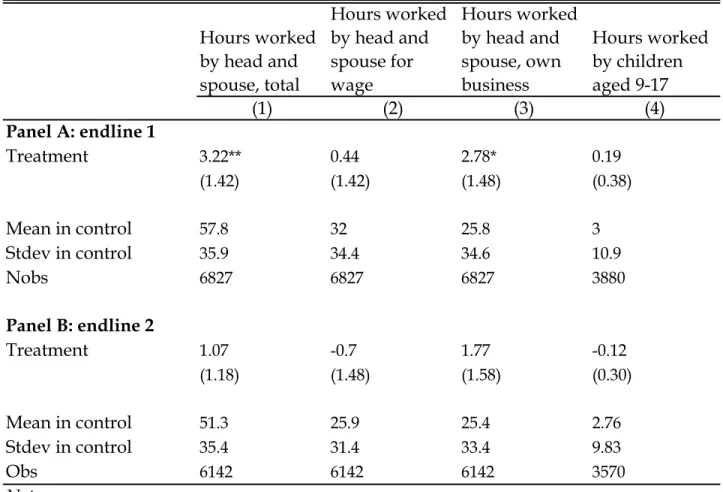
Table 8 shows the impact of the program on labor supply. In endline 1, adults (head and
spouse) in treatment households increase their overall labor supply by an average of 3.22 hours.
of hours worked for wages: those hours may be much less elastic, if the households do not
fully choose them. However, unlike Augsburg et al. (2012), we do not find the increase in
teenagers’ labor supply that is sometimes feared to be a potential downside of microfinance (as
the adolescents are drawn into the business by their parents). By endline 2, as control households
have started borrowing, the difference between treatment and control disappears.
4.4 Microfinance as social revolution: education, health, and women’s
em-powerment?
The evidence so far suggests a different picture from the standard description of the role of
microfinance in the life of the poor: the pent-up