The Impact of Trade Liberalization on Household Welfare and Poverty in India

Full text

(1)MPIA Working Paper 2006-01. The Impact of Trade Liberalization on Household Welfare and Poverty in India. Basanta K. Pradhan Sahoo Amarendra. January 2006. Basanta K. Pradhan (NCAER, New Delhi, India)) b.pradhan@warwick.ac.uk Sahoo Amarendra (Tilburg University, The Netherlands) amar_sahoo@hotmail.com. IDRC photo: N. McKee. 1.

(2) Abstract. A 28-sector, 3-factor and 9-household group Computable General Equilibrium (CGE) model for India is constructed to analyze the impacts of Tariff and Non-tariff Barriers (NTBs) on the welfare and poverty of socio-economic household groups. A general cut in tariffs leads to a decrease in overall welfare and reduction in poverty, which urban households are in a relatively better position to address. The choice of a fiscal compensatory mechanism with indirect tax on domestic consumption does not substantially change the pattern of impact except that it increases overall poverty in the economy. On the other hand, quota reductions on agriculture and food products result in a gain in welfare and a bigger reduction of poverty, with rural households doing better than urban households.. Keywords:. Computable general equilibrium (CGE) model, microsimulations, international trade, poverty, India.. JEL classifications:. D33, D58, E27, F13, F14, I32, O15, O53. This paper forms part of a MIMAP-India Project funded by International Development Research Centre (IDRC), Canada. The authors are thankful to Bernard Decaluwé, John Cockburn and Veronique Robichaud for their suggestions and comments on the CGE model.. 2.

(3) 1. Introduction In the face of serious internal and external imbalances, many developing countries, including India, have recently gone through a variety of structural adjustment programs. For India, major policy changes took place in the beginning of the 1990s. The biggest challenge of India's economic reform program has been the liberalization of its trade sector. Before the 1990s, India's trade policy regime was marked by a high level of tariff and non-tariff barriers, notably quantitative restrictions and various types of import licenses. To make India's trade more competitive internationally, policy makers have been struggling to keep trade restrictions to a minimum. Although the macro implications of these reforms have been studied, their impacts at the household level, which are of great concern to any society, are not well analyzed. Given the heterogeneity of India’s population and household groups, the impacts of trade reforms on their welfare and poverty are not expected to be uniform. Furthermore, although India has had an impressive record of growth since the late 1980s, it still faces massive challenges in terms of poverty and inequality. A World Trade Organisation (WTO) directive has forced the Indian government to focus on the elimination of import barriers in several key sectors. On April 1st 2001, the government announced its Export-Import Policy (EXIM-Policy), which removed quota restrictions from the remaining 715 goods covered. Major products in this list include food products and motor vehicles. In this paper, a computable general equilibrium (CGE) model is constructed in order to analyze the impact of major trade reform issues, viz. the removal of non-tariff barriers (NTBs) and reduction of tariffs on the income, consumer prices, welfare, and poverty levels of different household categories. The poverty line is endogenized in the model to take account of changes in consumer prices. The paper is divided into five sections. Section 2 portrays the Indian economy and highlights trade policy changes. The CGE model and benchmark data are discussed in Section 3. In Section 4, poverty analysis in a CGE framework is briefly described, while simulation results are analyzed in Section 5. Concluding remarks are given in the last section.. 3.

(4) 2. The Indian Economy, Trade Liberalization and Poverty 2.1 The Indian Economy and Policy Reforms• Since the 1960s, India has experimented with various policies in response to economic shocks in the context of a planned economy. For example, the impact of the unprecedented drought of 196567 on real GDP growth and the balance of trade was minimized through orthodox policies. However, there was a high level of inflation - almost 14-15 percent per year - because of loose fiscal and monetary policies. From 1967 to 1973, a number of changes were introduced. Export promotion measures, aiming to counteract the effect of the economy’s first devaluation in 1966, together with import restrictions, improved the trade balance and ultimately led to a trade surplus in 1972-73. During this period, the growing public deficit was financed by money creation. There were two shocks in the 1970s: A prolonged agricultural slump from 1972 to 1976, followed by the first oil crisis. The post-1973 period may be characterized as a period of orthodox stabilization. The foreign exchange constraint was the main problem on the demand side. A world recession in 1980-81 followed the oil shock in 1979-80. Foreign aid did not come easily because of adjustment policies that were underway in other countries. The 1979-80 period saw a rise in the fiscal deficit, which was again financed largely by money creation. India then approached the International Monetary Fund (IMF) and the liberalization process took place in a more systematic manner. Fiscal adjustments were made in order to finance the deficit through both domestic and foreign borrowing. Additionally, the eighties were the most turbulent period in the world’s foreign exchange markets: there was a sharp appreciation of the US dollar such that the Rupee underwent a 35% depreciation against the US Dollar between 1980 and 1985. In spite of all these policies, there was a worsening of fiscal and current account balances due to unchecked government expenditure. The increasing fiscal deficit was financed through borrowing and money creation. This eventually forced policy makers to conduct demand management in order to ease spiraling inflation, particularly by controlling money supply and toning down public spending. However, this austerity program came primarily through a reduction in its capital expenditure. The principal method for reducing the current account deficit during the second half of the eighties was to manage the rupee’s depreciation. Consequently, from 1985 to 1990, the nominal and real effective exchange rates depreciated by nearly 50 and 30 percent respectively. The carryover crisis from the late eighties, together with the Gulf war in the beginning of 1990s, pushed the Indian economy to an unprecedented level of crisis. This took the form of (a) high •. This section is based mainly on reports of various committees of the Government of India, which are referred. 4.

(5) (two-digit) inflation, (b) acute balance of payments disequilibrium, (c) huge fiscal deficits and (d) a rapid increase in external debt. With the objective of improving efficiency, productivity and global competitiveness, both macro and microeconomic reforms were introduced in the country’s industrial, trade and financial policy regimes. For a long period, Indian industries were characterized by inefficiency, high costs and uneconomical means of production with pervasive government control. The industrial policy of 1991 abolished industrial licensing while another major achievement was the abolition of the special permission needed under the Monopolistic and Restrictive Trade Practices Act (MRTP, 1969) for any investment and expansion. In response to the huge losses of public sector units (PSUs), the government took major steps to divest and restructure them. With the objective of addressing fiscal imbalances, reforms included correcting present irrationalities in the tax policies and a more cost-effective management of expenditure. Expenditure reform in India is crucial in view of high government spending and deficit. Agriculture and social sectors account for the majority of government subsidies targeting fertilizer, food, credit, higher and elementary education, etc. In agriculture, there was a shift in the allocation of public expenditure from subsidies to the creation and maintenance of infrastructure. Food subsidies, under the Public Distribution System (PDS), were revamped to target the poorest segments of the population. Both direct and indirect tax reforms were introduced with the objective of widening the tax base, increasing enforcement and equity, and developing a globally competitive economy. Direct tax rates were reduced. Reductions in customs duties, along with changes in excise taxes, played a crucial role in moderating domestic prices. Nevertheless, government revenue collection, as a percentage of GDP, remained stable in the late nineties. Sales taxes and excise duties contributed the most to government revenue and experienced the highest growth rate. Customs revenue, as a percentage of GDP, remained more or less stable. Overall, the growth rate in government revenue collection increased until 1995-96, followed by a drastic reduction in 1997-98 and again in 1998-99 (Table 1). This was, again, mainly due to fluctuations in the customs and excise collections. The major restructuring of the indirect tax system involved a reduction in excise duties even at the risk of losing substantial amount of revenue. The argument in support of this reform was that it would lead to greater efficiency in production, which would contribute to economic growth. Excise duties on major consumption goods were reduced. Broadly speaking, necessities of life like food, pharmaceuticals and footwear, as well as capital goods, are either exempt or bear a low rate of excise duties, semi-luxuries are moderately taxed, and luxuries support high tariff rates. to in the references list.. 5.

(6) Table 1: Percentage Change and Share of Different Taxes in Government Revenue. Income & Corporation Tax Customs duties Union Excise Duties Sales Tax Others Total Revenue Income & Corporation Tax Customs duties Union Excise Duties Sales Tax Others Total Revenue. 1993-94 1994-95 1995-96 1996-97 1997-98 1989-99 1999-00 Share of GDP at factor cost 2.46 2.83 3.01 2.97 2.67 3.00 3.23 2.84 2.93 3.35 3.46 2.89 2.64 2.82 4.06 4.09 3.77 3.64 3.45 3.29 3.57 3.60 3.63 3.34 3.41 3.28 3.22 3.46 2.66 2.69 2.96 2.68 3.04 2.85 3.11 15.61 16.17 16.42 16.17 15.33 15.00 16.19 Share of total government revenue 15.73 17.48 18.30 18.40 17.42 20.00 19.97 18.20 18.12 20.40 21.42 18.87 17.59 17.42 25.99 25.26 22.93 22.50 22.51 21.94 22.05 23.07 22.47 20.37 21.11 21.37 21.45 21.34 17.01 16.66 18.00 16.58 19.83 19.02 19.22 100 100 100 100 100 100 100. Source: Government of India, 1999.. One perennial problem of the Indian excise system has been the taxation of raw materials and intermediate inputs and the resulting cascading effect on the prices of final products. Imposing a value added tax (VAT) minimizes distortions. In India, the VAT has been introduced in the form of a modified value added tax (MODVAT), which provides for complete reimbursement of excise duties paid on raw materials and intermediate inputs used at various stages of production of final goods. Initially, the MODVAT scheme covered only a few items, but it has gradually been extended to a wide range of final manufacturing goods. Beginning in 1994-95, input tax credits were extended to capital goods. In its ideal form, a VAT is collected on the basis of value added at each stage of production and distribution. Since the cumulative effect of input taxation is absent under a VAT, the impact of this tax on production cost is limited. By avoiding distortionary cost escalation, it promotes the competitiveness of domestic industries in the world market. However, its operation has certain limitations in a developing country like India. In principle, a VAT should be imposed at a uniform rate at all stages of production and distribution, so that tax credit claims can be made easily. However, the MODVAT tends to be regressive. To ensure progressiveness, one needs to impose special excise duties on selected luxury items without the advantage of tax credits. On the other hand, exemptions should be extended to necessities only. A sales tax is normally an ad valorem levy imposed on consumers. In many cases, producers also come in its ambit if it applies to intermediate inputs. In India, there are a large number of sales tax rates and, in most cases, commodities that are subject to sales tax are also subject to excise duties. Some state governments have tried to reduce sales tax rates on some of the important commodities such as 6.

(7) capital goods and intermediate goods. In order to lessen distortions, the number of tax rates was reduced. States have also attempted to extend sales taxes to services in order to increase their revenue. Recently, there has been considerable progress towards the equalization of sales tax rates across states. Income tax is a tax on aggregate incomes from various sources. Before the start of the reform process the Indian income tax system was very complicated with many different rates. Subsequently, personal income tax rates were restructured with lower taxes, fewer rates and higher exemption limits. The maximum marginal individual income tax rate was reduced from 56% in 1991-92 to 40% in 199495; currently it is at 30%. It could be argued that these changes have led to “Laffer-type” revenue effects; i.e. a reduction in tax rates resulting in an increase in revenue. Currently, attempts are being made to bring most income earners under the umbrella of income tax. Reductions in income tax would leave households with more disposable income and thus generate more consumption demand and more savings in the economy. The Indian economy showed a recovery in its growth rate after the downturn in 1997 when it was only 4.8 percent (GDP), mainly due to the Asian Crisis. It was 6.6 percent in 1998-99, 6.4 percent in 1999-00 and 6.0 percent in 2000-01. Despite this near stagnancy in growth rates for two consecutive years, the Indian economy has shown remarkable resilience in the context of a substantial rise in the international price of crude oil. The slowdown in growth could chiefly be attributed to a decline in the growth of the service sector and slow growth in agriculture.. 2.2 Recent Trade Reforms In the pre-reform period, India's trade was marked by heavy reliance on quantity restrictions (QRs) and high import tariffs and surcharges aimed to protect local producers and contain the balance of payment deficit. Until the 1970s, India followed restrictive trade policies in order to regulate the current account deficit. In the process, it relied more on quantitative restrictions than on tariffs. A move towards the liberalization of India’s trade policy regime was made during the late 1970s and gained momentum during the latter half of the 1980s. In the mid-1980s, there were many important policy changes that took place in almost all sectors of the economy: industrial, foreign trade, monetary and long term fiscal policy (LTFP). Various committees, such as those led by Government of India in 1978, 1984 and 1985 emphasized two major points: (i) the need to develop an efficient system to render exports less costly and more profitable; and (ii) the need to move away from a discretionary system of quantitative import controls to a system based on tariffs. The LTFP envisaged an eventual removal of import licensing on all imports except consumer goods and also proposed a simplification of the complex tariff structure. Quantitative restrictions were gradually removed and tariffs reduced. Although QRs were not removed, they were simplified. A number of items for capital and 7.

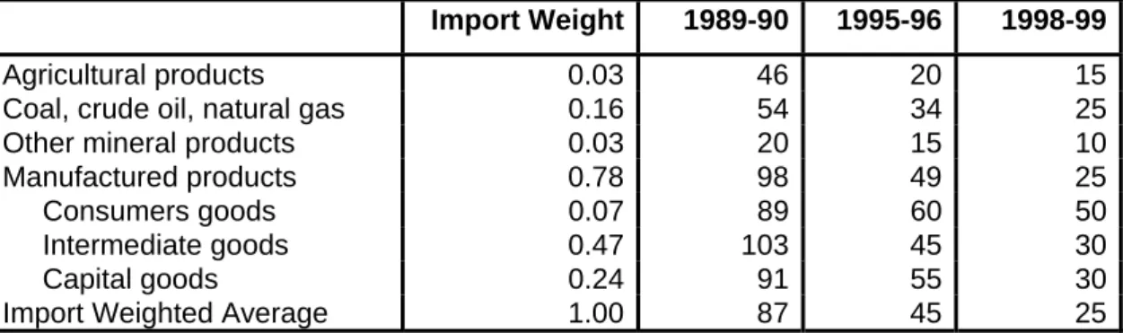
(8) intermediates goods became freely importable under Open General Licenses (OGL). According to some trade experts, as there were no domestic substitutes for items listed under the OGL, lifting of these QRs had little impact on import competition with domestic production (Srinivasan, 1998). Various types of licenses were issued in the pre-reform period: (a) Open General License, (b) Automatic License, (c) Supplementary Import License, and (d) Imports License for government-owned agencies. The beginning of 1991 was marked by a trend towards more liberal trade policy with the objectives of export-led growth, improved efficiency and competitiveness. The QR coverage was 94 percent for agricultural and 90 percent for manufactured intermediate and capital goods (Chadha, et al., 1999). As a result, India’s import-weighted average tariff was as high as 87% in 1989-90. The rapid increase in import tariffs in the latter half of the 1980s led to inefficient resource allocation. The Tax Reforms Committee proposed that the import-weighted average duty rate should be reduced to 45% in 1995 and further to 25% by 1998-99 (Government of India, 1993). It was suggested that average tariff rates on imports of intermediate and capital goods should be brought down drastically from 103 and 91, respectively, in 1989-90 to 30 in 1998-99. It was further suggested that additional protection might be given to new industries and new technologies.. Table 2: Proposed Tariff (Import Weighted Average) Import Weight. 1989-90. 1995-96. 1998-99. 0.03 0.16 0.03 0.78 0.07 0.47 0.24 1.00. 46 54 20 98 89 103 91 87. 20 34 15 49 60 45 55 45. 15 25 10 25 50 30 30 25. Agricultural products Coal, crude oil, natural gas Other mineral products Manufactured products Consumers goods Intermediate goods Capital goods Import Weighted Average Source: Government of India, 1993.. These policy reforms led to the reduction of the average (un-weighted) applied tariff rate from 125% in 1990-91 to 35% in 1997-98. The import-weighted average rate was reduced from 87% in 1990-91 to 20% in 1997-98. The highest rate of duty declined from 335% in 1990-91 to 45% in 199798 and to 40% in 1999-00. The highest protective customs tariff rate was scaled down further to 35% in 2000-01. It is noted that tariffs on consumer goods were drastically reduced as compared to tariffs on intermediate and capital goods.. 8.

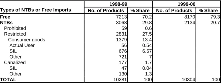
(9) Table 3: Tariff Structure of India (per cent) 1990-91 1993-94 1995-96 1996-97 1997-98 1999-00 2000-01 Average unweighted (whole economy) 125 71 41 39 35 Average weighted (whole economy) 87 47 25 22 20 Consumer goods 153 86 36 33 25 Intermediate goods 77 42 22 19 18 Capital goods 97 50 29 29 24 Maximum tariff rate 355 85 50 52 45 40 35 Source: As quoted by Chadha et al., 1999. Government of India, 2000. With respect to non-tariff barriers, the coverage of the Open General License was extended and the restricted list was cut drastically. There is a negative list of items, which does not fall under OGL. The negative list of imports consists of (i) prohibited items: items not permitted to be imported, (ii) restricted items: this includes consumer goods and special import licenses (SIL); and (iii) canalized items. The first stage of India’s reforms after 1991 continued to focus on the manufacturing sector while the agricultural sector was largely ignored. The share of value added in the manufacturing sector protected by QRs declined from 90 to 36 percent by May 1992 (Pursell, 1996). The corresponding decline was much smaller in agriculture, declining from 94 to 84 percent by May 1995. The import of 40 percent of agricultural products was still restricted since these were classified as consumer goods. The import of some restricted items was liberalized by permitting their imports through freely transferable Special Import Licences (SILs). SIL coverage has been extended systematically since April 1999, freeing various items by transferring them from restricted classification to the SIL list and from the SIL list to the OGL list. Various items have also been decanalized. Some of the newly freed categories, which were in the most restricted groups, were agricultural products and consumer goods. Table 4: Different Types of NTBs on India's Imports Types of NTBs or Free Imports Free NTBs Prohibited Restricted Consumer goods Actual User SIL Other Canalized SIL Other TOTAL. 1998-99 1999-00 No. of Products % Share No. of Products % Share 7213 70.2 8170 79.3 3068 29.8 2134 20.7 59 0.6 2831 27.5 1379 13.4 56 0.54 676 6.57 721 7 177 1.7 47 0.04 130 1.3 10281 100 10304 100. Source: Mehta and Mohanty, 1999.. 9.

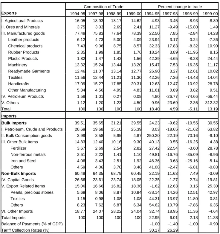
(10) It is estimated that, in 1998-99, there were no NTBs on 7,213 products out of 10,281 products at the 10-digit HS-ITC level (Mehta, 1999). The number of products on the 'Restricted items' list represented 27.5 percent of the total, while only 1.7 percent of products were 'canalized' (Table 4). With India's ExportImport (EXIM) Policy for 1999-00, 957 products were added to the free list, while only 2,134 products were subjected to some type of NTB. According to the estimation of an index of the coverage ratio of NTBs by different sections (21 commodity groups) of the HS classification for 1998-99, more than 90 percent of India's imports of manufacturing goods are not subjected to any type of NTB (Appendix-III). It is believed that India has been maintaining QRs on imports on balance of payments grounds. However, the United States of America filed a case with the WTO Dispute Body (DSB) against these QRs in May 1997. The DSB ruled against India and found that India's QRs on imports were not justified on these grounds. It recommended that India bring its import regime into conformity with WTO agreements to phase out these QRs by 2001. Of the 2,714 import lines at the eight-digit level of the HT-ITC classification on which such QRs were applied in 1997, the Government has been unilaterally liberalizing these imports. The EXIM Policy 2001 declared that QRs on the last batch of 715 items had been removed. A 20% devaluation of the rupee in July 1991 and the introduction of Exim licenses also marked the beginning of trade policy reform. These licenses were allotted to exporters as import entitlements against the value of exports and were freely tradable. In 1992, this system was replaced by a dual exchange rate mechanism with partial convertibility. In 1993, the economy moved into a unified exchange rate system. Since 1992, import licensing had been virtually abolished. In order to stimulate exports, a value-based advance license was introduced to permit duty-free imports of necessary raw materials and intermediate inputs up to a given share of export values. The Export Promotion of Capital Goods (EPCG) scheme was further liberalized to allow imports of capital goods at reduced customs duty rates.. 2.3 India's International Trade Trade policy reforms have helped to strengthen export performance and to improve competitiveness. Exports in US dollars experienced a significant recovery in 1999-00, attaining 13.2 percent, after negative growth in 1998-99 (Table 5). Although the value of imports has gone up substantially, growing by 2.2 percent in 1998-99 and 11.4 percent in 1999-00 due primarily to an increase in international crude oil prices, the current account deficit was contained at 0.9 percent of GDP in 1999-00. Growth in exports was mainly driven by a substantial increase in India's principal exports: handicrafts, textiles and 'chemicals and allied products'. However, the export of agricultural products, which also represents a significant share (14.8 percent) of India exports, fell for two consecutive years.. 10.

(11) Table 5: Structure and growth of India's main commodity exports and imports (US$) Composition of Trade Exports. 1994-95 1997-98 1998-99. I. Agricultural Products. Percent change in trade 1999-00 1994-95 1997-98. 1998-99. 1999-00. 16.05. 18.93. 18.17. 14.62. 4.93. -3.45. -8.93. -8.89. 3.75. 3.03. 2.69. 2.41. 11.27. -9.49. -15.80. 1.49. III. Manufactured goods. 77.49. 75.83. 77.64. 78.39. 22.50. 7.85. -2.84. 14.28. Leather products. 6.12. 4.73. 5.00. 4.09. 23.94. 3.17. 0.24. -7.36. Chemical products. 7.43. 9.06. 8.75. 8.57. 32.33. 17.83. -8.32. 10.90. Rubber Products. 2.35. 1.99. 1.85. 1.76. 18.24. 3.89. -11.95. 8.15. II. Ores and Minerals. Plastic Products Machinery. 1.82. 1.47. 1.42. 1.56. 42.39. -4.65. -8.28. 24.44. 13.32. 15.24. 13.44. 13.20. 15.47. 7.53. -16.35. 11.17. Readymade Garments. 12.46. 11.07. 13.14. 12.77. 26.90. 3.27. 12.61. 10.02. Textiles. 11.56. 12.44. 11.21. 11.30. 42.26. 7.36. -14.48. 14.04. Handicrafts. 17.09. 15.27. 17.85. 20.31. 12.63. 12.47. 10.92. 28.78. 5.34. 4.56. 4.99. 4.83. 11.61. 0.89. 3.82. 9.51. IV. Petroleum Products. 1.58. 1.01. 0.27. 0.08. 4.80. -26.77. -74.66. -66.44. V. Others. 1.12. 1.20. 1.23. 4.50. 9.96. 23.69. -2.36. 312.32. Total. 100. 100. 100. 100. 18.40. 4.59. -5.11. 13.19. Bulk Imports. 39.51. 35.65. 31.21. 39.55. 24.23. -9.62. -10.55. 30.55. I. Petroleum, Crude and Products. 20.69. 19.68. 15.10. 25.39. 3.03. -18.65. -21.62. 63.82. Other Manufacturing. Imports. II. Bulk Consumption goods. 3.99. 3.58. 5.95. 4.87. 250.20. 22.19. 70.16. -9.10. III. Other Bulk Items. 14.83. 12.40. 10.16. 9.30. 40.13. 0.55. -16.25. 4.38. Fertilizer. 3.67. 2.69. 2.54. 2.82. 27.42. 22.54. -3.60. 28.78. Non-ferrous metals. 2.51. 2.22. 1.41. 1.10. 49.81. -16.76. -35.09. -8.96. Iron and Steel. 4.06. 3.43. 2.51. 1.92. 46.36. 3.68. -25.16. -5.14. Others. 4.59. 4.06. 3.70. 3.46. 41.08. -2.47. -6.81. -0.83. Non-Bulk Imports. 60.49. 64.35. 68.79. 60.45. 22.19. 11.63. 7.49. -3.09. IV. Capital Goods. 26.66. 23.61. 23.74. 18.05. 22.35. -1.27. 2.74. -19.81. V. Export Related Items. 15.06. 16.66. 16.82. 18.36. -1.62. 12.63. 3.15. 25.30. 5.69. 8.06. 8.87. 10.94. -38.14. 14.26. 12.51. 42.97. Pearls, precious stones Textiles. 1.15. 0.98. 1.08. 1.08. 44.31. 13.97. 11.80. 0.81. Others. 8.23. 7.62. 6.87. 6.34. 54.62. 10.79. -7.86. 6.35. VI. Other Imports. 18.77. 24.07. 28.22. 24.04. 32.74. 18.95. 11.36. -4.64. 100. 100. 100. 100. Total Imports. 22.95. 6.01. 2.18. 11.38. Balance of Payments (% of GDP). -1.00. -1.40. -1.00. -0.90. Tariff Collection Rates (%). 30.17. 26.29. Source: Compact Disc of Handbook of Statistics on Indian Economy, Reserve Bank of India (2001).. On the other hand, 'petroleum, crude and products' constituted the major share of imports followed by capital goods and 'pearls and precious stones'. There has been a particularly significant rise in import of crude oil and 'pearls and precious stones'. The sharp increase in export-related imports like 'pearls and precious stones’ could be attributed to the heightened sales overseas of gems 11.

(12) and jewelry during this period. However, import of capital goods declined by 19.81 percent in 1999-00 and its share also declined from 23.74 percent to 17.09 percent in the same period. This could reflect a declining investment demand in the economy.. 2.4 Recent poverty trends Since 1991, the beginning of the era of full pace economic reform, there has been a great deal of debate in India about the possible impact of these policies on the poor. If one looks at the head count poverty ratio for rural and urban India since 1983, it can be seen that rural poverty has always been higher than urban poverty (Table 6). Approximately 80 per cent of the total poor live in rural areas. In the pre-reform period until 1990, both rural and urban poverty declined. There has generally been a reduction in poverty throughout both the rural and urban areas. However, the reduction was sharp between 1993-94 and 1999-00 largely due to an increase in GDP growth rate, which many believe was induced by economic reforms in the 1990s.. Table 6: Poverty Head-count ratio for Rural and Urban from 1983 to 1995-96 and 1999-00 Year 1973-74 1977-78. Rural 56.4 53.1. Urban 49.0 45.2. 1983 1987-88 1993-94 1999-00. 45.7 39.1 37.3 27.8. 40.8 38.2 32.4 23.6. Source: Planning Commission (1998, 2002).. 3. The Model The model has 28 production activities and three factors of production, viz. labor, land and non-land capital (Appendix I). Households, the private corporate sector, the public sector and government are the agents. Households are classified into four rural categories and five urban categories (Appendix II). Other than the distinction between land and non-land capital, the key distinguishing feature of this model, as compared to the other models in this volume, is the inclusion of import quota restrictions. When there are quota restrictions on the import of a commodity, its domestic price rises in response to increased demand, as supply of the imported good in domestic market remains unchanged. Prices on the domestic market thus depend on the demand elasticity of substitution between domestic and imported goods. Government administers the auctioning of quota licensing to 12.

(13) importers. The price of the license is competitively determined by the difference between price of the good in the domestic market and its price in the international market, which is expressed as the tariff equivalent. This generates a rent that becomes part of government revenue. However, there is an exception in the case of the import of petroleum products. About 98 percent of these imports are under quotas, which are canalized through government agencies. Any shortage of domestic petroleum supply relative to domestic demand is compensated by increased imports. Government fixes the import price on the domestic market, which, at times, could be lower than the world price. To avoid the complications of modeling this mechanism, we assume that there is no rent on these imports in the benchmark. It is assumed that import demand is endogenously determined in the model and import price in the domestic market is exogenously fixed.. 3.1 Calibration and the Benchmark Equilibrium The Social Accounting Matrix (SAM) gives the benchmark equilibrium for the model. The SAM used for the present study is based on Pradhan, Sahoo and Saluja, 1999. The economy is classified into 28 production sectors to take care of important economic activities. Out of 28 sectors, ‘construction’, ‘electricity’, ‘education’ and ‘health’ are not importable sectors. Sectors that are not engaged in exporting activities are ‘crude oil and gas’, construction’, electricity’, ‘education’ and ‘health’. ’Food-grains’ has been separated from the rest of the agriculture sector for its vital role in poverty. Coal and lignite, and crude oil and natural gas are the two components of the primary energy sector. This sector requires higher investment in exploration and also, due to high domestic demand, a substantial amount of it is imported. The manufacturing sectors are divided in such a way that capital goods are separated from consumer items like ‘food articles and beverages’, ‘textiles’, etc. to take care of investment. Because of rapid economic development, ‘cement and other non-metallic mineral products’, which are basically inputs to the construction sector, are very important. Their growth gives a fillip to the crucial housing sector as well. ‘Fertilizers’ as a sector has a big role to play in influencing agriculture, particularly with respect to the recent debate concerning the withdrawal of fertilizer subsidies. ‘Petroleum products’ are kept separately as these are byproducts of one of the important energy sectors, ‘crude oil and natural gases’. They are also crucial energy sectors whose prices have been, until recently, administered by the government and have strong impacts on the economy. Even now, the market does not have a very big role in determining their prices. Moreover, their prices have recently gone up dramatically in international markets. Construction’ is a highly labor intensive sector. ‘Electricity’ is an important sector, with important linkages in the economy. ‘Infrastructure services’ and 13.

(14) ‘financial services’ have been kept as separate sectors as they play important roles, particularly in the context of liberalization. ‘Health’ and ‘education’ are mainly public goods and also influence welfare. Expenditure in these sectors by government, private institutions and individuals is considered as investment in human capital. Households are classified according to their principal sources of income. There are four rural and five urban occupational household groups. We note that 56% of rural income comes from agriculture while 97% of urban income comes from non-agricultural activities (Table 7). However, there are substantial differences among household groups within each of these areas. While rural agricultural households derive almost 90% of their income from agriculture, the rest of the rural household groups get almost 90% of their income from non-agricultural activities. Also, urban agricultural households derive 75% of their income from agriculture, whereas all other urban household categories derive almost all income from non-agricultural sources.. Table 7: Sources of income for household groups (as a percentage of Total income) HH Categories Rural Self Employed in Agriculture Self Employed in Non-agriculture Agriculture Wage Earners Non-agriculture Wage Earners Other households Total Urban Agriculture Households Self Employed in Non-agriculture Salaried Earners Non-agriculture Wage Earners Other Households Total GRAND TOTAL. Agriculture. Non Agriculture. Total. 87.12 12.87 88.52 10.32 12.53 55.66. 12.88 87.13 11.48 89.68 87.47 44.34. 100 100 100 100 100 100. 74.91 0.95 0.90 2.19 1.03 2.46 32.14. 25.09 99.05 99.10 97.81 98.97 97.54 67.86. 100 100 100 100 100 100 100. Source: Pradhan & Roy (2003) (MIMAP-India Survey (1996)) Note: The SAM used for this model, rural self-employed in non-agriculture and rural non-agricultural households are combined into one group as ‘'rural artisans’'.. 14.

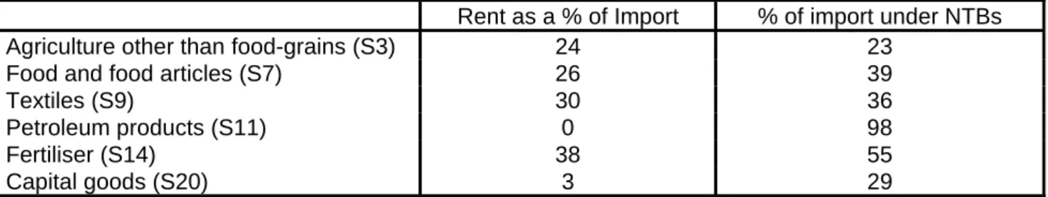
(15) Table 8: Benchmark Parameters1. Food grains Other agriculture (no quota) Other agriculture (with quota) Crude oil Other mining Food articles (no quota) Food articles (with quota) Textiles (no quota) Textiles (with quota) Traditional manufacturing Petroleum products (with quota) Petrochemicals Fertilizer (no quota) Fertilizer (with quota) Other chemical products Non-metallic goods Basic metals Metallic products Capital goods (no quota) Capital goods (with quota) Miscellaneous. manufacturing Construction Electricity Infrastructure services Financial services Education Health Other services Total. CES Import CET Export CES Production Average Tariff Elasticity Elasticity Elasticity Collection* 1.1387 0.92 0.78 1.1387 0.92 0.78 0.1792 1.1387 0.92 0.78 0.1740 1.6195 0 1.1 0.0006 1.6195 0.92 1.54 0.0186 1.1345 1.16 0.58 0.0471 1.1345 1.16 0.58 0.0445 3.082 2.49 0.77 0.1812 3.082 2.49 0.77 0.1824 2.8021 1.2 1.01 0.3139 2.0022 0.69 1.85 0.9961 5.6926 1.06 1.17 0.2998 2.6171 0.69 0.73 0.0118 2.6171 0.69 0.73 0.0116 2.6171 0.69 0.73 0.3597 2.8079 1.04 1.05 0.6627 1.4319 5.42 0.64 0.2588 3.6993 0.68 1.02 0.4145 2.3484 1.32 0.98 0.3185 2.3484 1.32 0.98 0.3334 1.9225 1.64 0.77 0.6551 0 0 1.1 0 0 2.26 2.145 0.92 1.45 2.145 0.92 1.65 0 0 1.08 0 0 1.08 2.145 0.92 1.08 0.3092. Source: Chadha, et al. (1998). CET elasticities of substitution are considered to be the same as export demand elasticities. *Authors' own estimation.. The tariff rates used in the benchmark are the actual collection rates, i.e. ratio of total value of import duties including additional duties to the value of imports. For the computation of the tariff equivalent due to non-tariff barriers, rent generated is computed using the wedge between value of imports of a sector on the domestic market and its value on the international market. There are six importing sectors which involve quota restrictions, viz. 'agriculture products other than food-grains', 'food and food articles', ‘textiles’, ‘petroleum products’, ‘fertilizer’, and ‘capital goods’ (Table 9). Imports of each of these sectors are divided into two parts - one that comes through quota restriction and the 1. Benchmark parameters are given for 23 sectors. Because of a lack of detailed information, the sectors with quota are created as a proportion of their import shares in the original import sectors. We assume that their behavioural parameters are the same as those in their original sectors.. 15.

(16) other that is freely imported. Out of these six sectors, imports of 'petroleum products' are fully canalized through government agencies. It is assumed that this sector does not generate any rent. Table 9: Benchmark quota rent and non-tariff barriers (in 1994-95) Agriculture other than food-grains (S3) Food and food articles (S7) Textiles (S9) Petroleum products (S11) Fertiliser (S14) Capital goods (S20). Rent as a % of Import 24 26 30 0 38 3. % of import under NTBs 23 39 36 98 55 29. Source: Authors' own calculations based on McDougall et al., 1998. The latter gives the price wedges of different imported commodities, i.e. difference between value of imports at the domestic market price and value of the same at the world price (in dollar terms).. In the linear expenditure system (LES) demand functions, the values of marginal budget shares and minimum consumption parameters have been estimated with the help of micro household data taken from MIMAP Household Survey (1996), conducted by the National Council of Applied Economic Research (NCAER), New Delhi. In the benchmark, the minimum consumption parameters are calibrated with the use of these budget shares and the ‘supernumerary income ratio’2 for each household.. 4. Policy Simulations This paper attempts to capture the poverty and welfare impacts resulting from India’s recent sweeping trade reforms. The main objectives of the trade reforms have been to accelerate the growth of the economy by removing the distortions. The policy changes have undoubtedly impacted on the households by affecting their income and consumption levels, and hence, their welfare and poverty. In order to look into the above issues, the following simulation exercises have been carried out in the model3. SIM1: Complete removal of import tariffs across the board without any compensating mechanism regarding government revenue. SIM2: Quota restrictions on imports of 'other agriculture not inclusive of food grains' (S3) and 'food and food articles' (S7) are relaxed, i.e. their import quota limits are increased by 40 per. 2. The supernumerary income ratio measures the amount of available spending power that consumers have over and above the minimum consumption level. For details see Taylor, 1990.. 16.

(17) cent; no compensating mechanism with respect to government revenue. SIM3: Complete removal of import tariffs and an increase in the uniform indirect tax rate on domestic demand to keep government revenue constant.. Completely doing away with import tariffs in SIM1 makes imports cheaper, leading to an inflow of more imports. Lower import prices reduce the relative demand for domestic goods. The degree of change depends on the import elasticity of substitution, import intensity of the sector and the base line tariff. It is expected that sectors with high import intensity and high demand elasticity of import vis-àvis domestic goods would experience a greater increase in imports. However, it also depends on the tariff base of the sector. Sectors with higher tariffs respond more to the reduction in tariff rate. Sectors like 'traditional manufacturing' (S10), 'finished petrochemicals' (S12), ‘other chemicals’ (S15), 'nonmetallic products' (S16), ‘metallic products’ (S18) and ‘other miscellaneous industries’ (S21) have shown a significant rise in imports because of their high CES elasticity and high tariff base (see Table A1-sim1). It is also expected that a high import intensity, i.e. high share of imports relative to domestic consumption, will encourage a rise in imports when tariffs fall. Crude oil and natural gas’ (S4), ‘other mining and quarrying’ (S5), ‘non-quota food products’ (S6), ‘petroleum products’ (S11), and all the service sectors have a small response to tariff reductions because of either low import intensity or a very low tariff base4. Sectors faced with import quotas, i.e. ‘other agriculture’ (S3), ‘food products’ (S7), ‘textiles’ (S9), ‘petroleum products’ (S11), ‘fertilizer’ (S14), and ‘capital good’ (S20) show no gain at all in the volume of imports. With fixed foreign exchange reserves, resources are drawn from these sectors in order to finance imports in other more responsive sectors. With our assumption of a fixed current account, a decline in overall imports leads to a depreciation of the real exchange rate, which encourages exports. It again depends on the elasticity of transformation between the supply of goods to the domestic and export markets as well as exportintensity, i.e. the ratio of exports to domestic supply. Exports from most sectors increase, notably for ‘basic metals’ (S17) and ‘textiles’ (S8 and S9), which have high export elasticities. The lower cost of imports is expected to reduce domestic production due to lower domestic demand. However, this does not happen for some industrial sectors (from S4 to S13) because of their increase in local demand and also in exports, which is the consequence of the overall decline in purchase prices. The fall in import prices results in a decrease in production prices because of lower input prices. The rest of the sectors, including agriculture and services, lose their comparative advantage due to tariff removal. Change in the production activities in the economy results in a 3. Results of the simulations are given in the Annexes’ tables.. 17.

(18) reallocation of factors of production. All the factors of production suffer from a decline in their remuneration, notably non-land capital (see Table A2-sim1). There is an overall decline in factor remuneration. All household groups suffer heavily in terms of declining nominal incomes (see Table A3-sim1). This is mainly because of the contraction in the major domestic sectors and fall in prices. The welfare impacts on the different household groups depend on their real consumption, which is affected by the composite prices of the commodities as well as their disposable income. There is an across-the-board decline in these prices. The largest decline is observed in industrial products because of their relatively high composition of imports. Consumer price indices for different household groups, which determine the real consumption of households, also decline (see Table A4sim1). Equivalent variations, as a measure of welfare, decrease for all rural and urban household groups except rural ‘agriculture labour’ and ‘other household’ groups, and urban 'agriculture household’ and ‘other household’ groups (see Table A5-sim1). Though there has been a decline in consumer prices, there is an overall welfare loss for rural as well as urban households in the economy due to the overwhelming impact of the fall in their net disposable income. The drop in household disposable income is the result of a decrease in relative factor rewards and government transfers to households. Government loses revenue due to tariff removal and hence, there is a squeeze in transfer payments to households. However, the poverty ratio eases up for both rural and urban household groups. This decline could be attributed to the larger impact of the decrease in consumer prices, which reduces the poverty line. Given the undistorted income distribution, the lowering of the poverty line pushes the marginal households out of poverty. Households in the rural areas gain more in terms of the increase in welfare and decrease in poverty than urban households following the complete removal of import tariff. In Simulation 2 (SIM2), reducing quota restrictions on ‘agricultural products’ (S3) and 'food and food articles' (S7) implies allowing more imports of these goods into the domestic market. The import intensities are low for agricultural products and food articles (see Table A6-sim2). This implies that demand for agricultural products is more biased towards those domestically produced in the base year. However, a shift in import demand also depends upon the elasticity of substitution in local demand between domestically produced and imported goods. As elasticity of substitutions are more than onet and almost the same for both S3 and S7, with relaxing of import restrictions on these items, domestic demand for their imports goes up significantly and almost equally. With more availability of hitherto quota-restricted goods, there is a fall in the domestic production of these goods. In order to model the imposition of quota restrictions, tariff equivalents, which are equal to the. 4. There are no tariffs on ‘food grains’ and service sectors.. 18.

(19) difference between domestic and international prices, are imposed on the importers in the model. When quotas are relaxed, this tariff equivalent, otherwise known as rent, decreases in both these sectors significantly. This, in fact, reduces the cost of imports. Hence, composite prices, i.e. prices faced by consumers, of these goods decline. Due to the relatively high import share of food articles (S7), import prices decline more in this sector than in other agriculture (S3). This leads to a significant decline in the composite price of food articles (see Table A9-sim2). Significantly lower import prices for these items, and their linkage to the other sectors in the economy, results in a decline in domestic purchaser prices and producer prices in almost all sectors (see Tables A6-sim2 and A9-sim2). With exogenously given foreign savings, an increase in imports of these goods leads to a depreciation of the exchange rate, i.e. domestic currency becomes cheaper in terms of the US dollar. Imports are withdrawn from the rest of the sectors to finance quota imports. There is overall increase in exports due to depreciation (see Table A6-sim2). Agriculture sectors suffer from the decline in production due to high imports in these sectors. However, industry and service sectors generally increase production due to lower domestic input prices as well as an increase in exports. The lower cost of production, reflected in the value added prices, results in a lowering of remuneration to all factors of production (see Table A7-sim2). However, labour and land suffer relatively more from the lowering of factor rewards due to the shrinkage of domestic agricultural activities. Hence, we might expect that rural household groups would be worst hit. However, there is a marginal rise in other income due to the rise in transfer income from government to households (see Table A8-sim3). The rise in government revenue, as a result of increased domestic activities, contributes to the increase in transfer payments to households. In general, rural and urban household groups almost equally suffer in terms of the decline in nominal disposable income. It is observed that the effect of the reduction in quantitative restrictions on imports of food and agricultural items is positive on the households. Welfare is based on the real consumption of households, which is affected by the change in consumer price indices. There has been a decline in consumer price indices for all household groups (see Table A10-sim2). The decline is greater for rural households due to the lower purchaser prices of agricultural products, which in turn is a result of the relaxation of quotas to the domestic market. Welfare increases for almost all household groups except for the rural ‘agricultural self-employed’. In fact, welfare increases marginally more for rural households. Poverty ratios decline more in the rural area than in the urban areas. This is a result of the dominant role of the decrease in consumer prices over the decline in relative income due to quota removal. Only the ‘agricultural self-employed’ and ‘agricultural labour’ households groups, in rural areas, the ‘salaried class’ in urban areas experience a decline in poverty. In Simulation3 (SIM3), tariffs are removed completely and there is an increase in domestic 19.

(20) indirect taxes to compensate for the loss in government revenue. In this case, the pattern of results is quite similar to Simulation1 (see Tables A11-sim3 to A15-sim3). But factor prices decline more than due to a rise in the cost of production following the compensatory increase in the indirect tax (see Tables A2-sim1 for Simulation 1 and A12-sim3 for Simulation 3). Despite the decline in prices, welfare is reduced for all household groups, even more than the reduction in Simulation 1 (see Tables A5sim1 for Simulation 1 and A15-sim3 for Simulation 3). However, unlike the first simulation, poverty ratios increase for all household groups (see Table A15-sim3). Here, the decline in income dominates the decrease in consumer prices to raise the poverty ratio. Also, unlike the first simulation, households in rural areas experience a larger decline in welfare and a larger increase in poverty than urban households.. 5. Conclusion In the Indian economy, trade policies significantly affect the prices, demands and growth in the economy. They affect the welfare and the poverty of household groups directly as well as indirectly. This paper is confined to some policy issues pertaining to non-tariff barriers (NTBs) on imports of agricultural products as well as on 'food and food articles', and import liberalisation through a general tariff reduction. Though our policy simulation regarding quota restrictions is confined to agriculture and food products only, quota reductions on these sectors are in line with the EXIM policy of India, 2001. Trade liberalisation, both in tariffs and in non-tariffs, promotes exports and hence, export-led growth. Overall welfare decreases in the case of a removal of tariff but increases for quota relaxation. However, poverty declines in both cases. Rural areas are in a better position than their urban counterparts in terms of welfare improvement. Both disposable income and consumer prices decline in both scenarios, but the decline in welfare is attributed to the dominant role of the change in income and the decline in poverty to the fall in prices. When we allow for a compensatory increase in indirect taxes along with tariff removal, overall poverty increases and welfare declines. In this case, rural household groups suffer more than urban households. Another policy implication emerging from our simulations is in the case of tariff elimination, where the removal of quota restrictions could be a prerequisite step in order to have a more positive price effect on the economy, which could lead to higher welfare gains for households.. 20.

(21) References Chadha, Rajesh, Sanjib Pohit, Alan V. Deardorff and Robert M. Stern (1998), The Impact of Trade and Domestic Reforms in India: A CGE Modeling Approach,Ann Arbor, University of Michigan Press. Chadha, R., D.K. Brown, A. V. Deardoff and R. Stern, 1999, “Computational Analysis of India’s Post1991 Economic Reforms and the Impact of the Uruguay Round and Forthcoming WTO-2000 Trade Negotiations”, WTO 2000: South Asia Workshop, NCAER-World Bank, New Delhi (Dec.20-21). Government of India (1978), “Report of the Committee on import-export Policies and Procedures”, Ministry of Commerce, New Delhi. Government of India (1984), “Report of the Committee on Trade Policies”, Ministry of Commerce, New Delhi. Government of India (1985), “Report of the Committee to Examine the Principles of a Possible Shift from Physical to Financial Controls”, Ministry of Finance, New Delhi. Government of India (1993), “Tax Reforms Committee: Final Report Part II”, Ministry of Finance, New Delhi. Government of India (1999), The Economic Survey 1999-2000, Ministry of Finance, New Delhi. Government of India (2000), The Economic Survey 2000-2001, Ministry of Finance, New Delhi. Government of India (2001), The Economic Survey 2001-2002, Ministry of Finance, New Delhi. Mehta, R. (1999), “Tariff and Non-tariff Barriers of Indian Economy: A Profile”, Research and Information System for the non-aligned and Other Development Countries (RIS), New Delhi. Mc.Dougall, R., A. Elbehri and P. Troung (eds.) (1998), "Global Trade, Assistance, and Protection: The GITAP 4 Data Base", Centre for Global Trade Analysis, Purdue University. Planning Commission (1998), Ninth Five Year Plan (1997-2002), Volume-I Planning Commission (2002), National Human Development Report, 2001. Pradhan, B.K. and P.K. Roy (2003), “The Well-Being of Indian Households: MIMAP-India Survey Report”, Tata-McGraw Hill Publishing, New Delhi. Pradhan, B.K., A. Sahoo and M. R. Saluja (1999), “A Social Accounting Matrix for India, 1994-95”, Economic and Political Weekly, November 27. Pursell, G. (1996), “Indian Trade Policies since 1991/92 Reforms,” (mimeo), World Bank, Srinivasan, T.N. (1998), "Foreign Trade Policies and India's Development", in Uma Kapila (ed.), Indian Economy since Independence, Academic Foundation, Delhi. Taylor, L. (1990), Socially Relevant Policy Analysis: Structuralist Computable General Equilibrium Models for the Developing World, Cambridge, Mass: MIT Press.. 21.

(22) APPENDIX I The whole Indian economy is divided into 28 sectors, 5 primary sectors, 18 secondary sectors and 5 service sectors. Agricultural Sectors S1. Food grains (Tradable) S2. Other agriculture (Tradable, no quota) S3. Other agriculture (Tradable with quota) Industries S4. Crude oil and natural gas (non-exported, but importable) S5. Other mining and quarrying: Coal and lignite, Iron ore and other minerals (Tradable) S6. Food products and beverages (Tradable, no quota) S7. Food Products and beverages (Tradable with import quota) S8. Textiles (Tradable, import quota) S9. Textiles (Tradable with import quota) S10. Other traditional manufacturing goods, viz. wood, paper and leather products (tradable) S11. Petroleum products (Tradable with import quota) S12. Finished petrochemicals (Tradable) S13. Fertiliser (Tradable, no quota) S14. Fertiliser (Tradable with import quota) S15. Other chemicals (Tradable) S16. Non-metallic products: cement and other non-metallic mineral products (Tradable) S17. Basic metal industries including iron and steel (Tradable) S18. Metallic products (Tradable) S19. Capital goods (Tradable, no quota) S20. Capital goods (Tradable with import quota) S21. Other miscellaneous manufacturing industries (Tradable) S22. Construction (non-tradable) S23. Electricity (non-tradable) Service Sectors: S24. Infrastructure services: gas and water supply, trade, transport, hotel and restaurants (Tradable) S25. Financial services: banking and insurance (Tradable) S26. Education (non-tradable) S27. Health (non-tradable) S28. Other services (Tradable, due to the Information Technology sector). 22.

(23) APPENDIX II Households. A. Rural Households. 1. RAGSLF: Rural Agricultural Self-employed) 2. RAGLAB: Rural Agricultural Labour 3. RNAG: Rural Non-agricultural Labour) 4. ROTH: Rural Other Households. B. Urban Households. 1. UAG: Urban Agricultural Households 2. UNAGSLF: Urban Non-agricultural Self-employed 3. USALARY: Urban Salaried Class 4. UNAGLAB: Urban Non-agricultural Labour (casual labour) 5. UOTH: Urban Other Households. 23.

(24) Appendix III: India's Import-weighted Average Tariff Rates and Non-tariff Barriers by Different Sections of HS Classification Import-weighted Average additional duties). Tariff. Live Animals: Animal Production Vegetable Products Animal or veg.fats & oils Prepared foodstuffs, Beverages Mineral Products Product of the Chemical Plastic & articles thereof Raw hides, skins, leather Wood & wood articles, wood Pulp of wood or other fibre Textle & textile articles Footwear, headgear, umbrellas Articles of some plaster Natural or cultured pearls Base Metals & articles of base Machinery & mechanical appliances Vehicles, aircraft, vessels Optical, photograph, cinematograph Arms & ammunition, parts Misc. manufactured articles Works of arts collector's pieces TOTAL. Rates. (including. 1993-94 89.55 112.46 85.00 104.74 101.40 91.11 368.97 75.25 85.43 83.98 117.48 85.01 94.39 85.00 96.31 102.13 85.17 86.15 85.00 85.68 81.86 102.34. Different Types of NTBS on India's Imports: 1998-99 (Rs. Crores) Free NTBs Not 1989-99 Total Value Per cent Value Per cent Estimable 22.38 31.81 85.35 5.46 14.65 5.94 43.21 24.28 2182.75 17.11 10577.41 82.89 5.29 12765.45 40.44 17.19 0.70 2453.36 99.30 598.59 3069.14 68.23 160.825 36.62 278.345 63.38 45.39 484.56 32.33 6358.81 25.41 18670.22 74.59 423.32 25452.35 38.69 12772.81 85.30 2201.94 14.70 355.25 15330 65.05 3592.84 95.78 158.25 4.22 151.67 3902.76 19.29 498.27 97.77 11.34 2.23 7.1 516.71 4.63 965.88 99.81 1.84 0.19 0 967.72 28.12 1719.22 60.65 1115.65 39.35 59.63 2894.5 52.40 1560.89 90.46 164.54 9.54 15.21 1740.64 50.80 108.51 99.58 0.46 0.42 0.36 109.33 55.81 404.44 95.64 18.45 4.36 16.34 439.23 50.80 43.19 0.31 14043.79 99.69 2.65 14089.63 47.29 11049.6 99.10 100.77 0.90 1062.73 12213.1 35.60 17121.66 95.40 826.48 4.60 2380.61 20328.75 38.08 3330.72 64.98 1795.09 35.02 149.58 5275.39 34.65 2088.49 98.36 34.72 1.64 19.11 2142.32 50.80 0 0.00 1.77 100.00 0 1.77 49.45 193.37 87.45 27.75 12.55 23.55 244.67 30 7521.44 99.99 0.6 0.007977 0 7522.04 38.13. Source: Mehta (1999). 1.

(25) Table 1: Indicators of protection Sectors Agriculture Mining Primary Food, beverages and tobacco Textiles and leather Wood, cork and products Paper and printing Chemicals, petrol and coal Non-metallic minerals Basic metal industries Metal products and machinery Other Manufacturing Secondary Total. Nominal Rate of Protection Effective Rate of Protection Quantitative Restrictions 1988-89 1995-96 SAM 1988-89 1995-96 SAM 1988-89 1995-96 1999-00 91.1 24.5 35.0 92.1 25.7 34.7 100.0 78.4 59.9 106.5 39.2 41.3 102.4 38.1 38.9 99.4 30.2 27.1 92.3 25.6 35.5 92.9 26.7 35.1 100 74.8 57.4 144.7 48.9 66.8 87.1 60.8 108.2 100.0 74.5 48.0 145.4 49.8 65.0 151.4 55.1 75.0 100.0 56.0 45.1 127.8 48.1 65.0 133.7 56.2 77.5 100.0 42.0 5.7 149.6 43.0 60.5 142.4 41.6 60.2 100.0 42.3 22.5 177.7 45.4 62.6 224.1 47.8 70.1 97.5 38.1 15.5 145.9 50.0 65.0 150.9 52.2 70.5 98.3 76.5 36.3 197.5 46.6 49.0 180.3 49.4 52.1 53.4 13.8 11.4 138.2 49.6 62.3 128.9 50.6 67.2 80.1 40.7 25.0 151.5 49.1 64.6 151.6 50.3 68.3 78.5 53.6 21.5 152.5 48.4 62.4 151.3 51.6 71.4 87.4 46.1 27.7 112.2 33.2 44.4 112.2 34.9 47.1 95.8 65.3 47.6. Source: Mihir Pandey, NCAER, 1998 (Revised, 2000). Notes: 1. SAM refers to the year of the SAM, which is 1994-95. 2. The years indicated are suggestions and can be modified according to data availability. 3. The sectors should correspond to the branches/products in your SAM. More lines can be added as required. 4. For quantitative restrictions, indicates if any products in the sector are affected or, preferably, indicate the coverage ratio (tariff lines affected/total tariff lines).. 2.

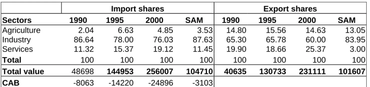
(26) Table 2: International trade. Sectors Agriculture Industry Services Total Total value CAB. 1990 2.04 86.64 11.32 100 48698 -8063. Import shares 1995 2000 6.63 4.85 78.00 76.03 15.37 19.12 100 100 144953 256007 -14220 -24896. SAM 3.53 87.63 11.45 100 104710 -3103. 1990 14.80 65.30 19.90 100 40635. Export shares 1995 2000 15.56 14.63 65.78 60.00 18.66 25.37 100 100 130733 231111. SAM 13.05 83.95 3.00 100 101607. Sources: 1. National Accounts Statistics, Government of India (2001) 2. Handbook of Statistics on Indian Economy, Reserve Bank of India (2001) Notes: 1. SAM refers to the year of the 1994-95. 2. The years indicated are suggestions and can be modified according to data availability. 3. The sectors correspond to the branches/products in SAM. More lines can be added as required. 4. Total value in Rs. Crores. 5. CAB = Current account balance in Rupees Crores.. Table 3: Government revenue (SAM year) Tariffs Direct taxes Production taxes Sales taxes Other revenues Total Total revenue Total expenditure Public deficit. 1985 19.93 13.75 30.06 18.48 17.78 100% 47805 44156 -3649. 1990 17.67 11.07 24.58 23.09 23.59 100% 116807 95379 -21428. 1995 15.29 15.99 20.40 25.21 23.11 100% 233821 195187 -38634. 2000 10.95 14.80 17.33 22.03 34.89 100% 436391 309531 -126860. SAM 18.55 25.90 12.21 35.15 8.20 100% 144414 180969 -36555. Source: National Account Statistics, Government of India (2001) Notes: 1. SAM is of the year 1994-95. 2. The years indicated are suggestions and can be modified according to data availability. 3. The sectors should correspond to the branches/products in your SAM. More lines can be added as required. 4. Total revenue, total expenditure and public deficit in Rs. Crores.. 1.

(27) Table 4: Average tax rates (SAM year) Sectors S1 S2 S3 Agriculture S4 S5 S6 S7 S8 S9 S10 S11 S12 S13 S14 S15 S16 S17 S18 S19 S20 S21 Industry S22 S23 S24 S25 S26 S27 S28 Services Total. Effective tariffs. Sales taxes 0.003 0.028 0.028 0.020 0.118 0.027 0.028 0.028 0.04 0.04 0.042 0.216 0.041. 0.174 0.174 0.139 0 0.018 0.045 0.045 0.182 0.182 0.336 0.988 0.323 0.012 0.012 0.375 0.817 0.265 0.441 0.333 0.333 0.753 0.326. Production taxes. 0.044 0.057 0.045 0.033 0.063 0.063 0.047 0.054 0 0.056 0.021 0.018 0.04 0.020 0.032. 0.290. Source: Based on Pradhan, Sahoo and Saluja (1999) Notes: SAM refers to the year of the SAM, which is 1994-95. For sectoral classification see Appendix 1.. 2. -0.048 -0.018 -0.018 -0.028 0.01 0.009 0.004 0.004 0.003 0.003 0.013 0.222 0.079 0.029 0.029 0.06 0.011 0.03 0.015 0.047 0.047 0.031 0.036 0.013 0.017 0.003 0.002 0 -0.002 0.008 0.006 0.010.

(28) Table 5: Sources of household income (1994-95r) Average Wage Capital Land Public Private Foreign Household Population income income income rent transfers transfers transfers* categories (shares) (values) (shares) (shares) (shares) (shares) (shares) (shares) Rur Cultivator 24.22 5324 13.36 20.46 78.49 34.61 2.68 Rur ag lab 22.08 3349 16.85 0.46 0.56 9.71 4.44 Rur Artisan 13.85 4927 10.01 14.81 15.50 13.04 3.49 Rur Other 14.76 6327 14.80 3.76 4.18 8.49 11.93 Urb farmer 1.24 5751 0.74 1.62 1.28 1.19 2.70 Urb nag self 5.40 11090 6.03 32.69 0.00 14.39 28.03 Urb salary 12.19 12814 34.34 14.26 0.00 11.88 23.32 Urb Casual Lab 2.81 5074 2.96 3.54 0.00 2.54 1.05 Urb Other 3.44 14946 0.90 8.40 0.00 4.16 22.35 Total 100% 100% 100% 100% 100% 100% 100% Total value Source: Pradhan & Roy (2003) * SAM for India, Pradhan, Sahoo and Saluja (1999) Notes: 1. SAM refers to the year of the 1994-95. 2. Total values and average income values in rupees.. Table 6: Poverty and Inequality. Headcount ratio RURAL URBAN Poverty gap RURAL URBAN Poverty severity RURAL URBAN Gini coefficient RURAL URBAN. 1983-84 44.50 45.70 40.80 11.96 12.32 10.61 4.61 4.78 4.07. 1987-88 38.90 39.10 38.20 9.32 9.11 9.94 3.26 3.15 3.60. 1993-94 36.00 37.30 32.40 8.30 8.45 7.88 2.79 2.78 2.82. 0.2976 0.3303. 0.2983 0.3537. 0.2819 0.3394. Source: Planning Commission (1998), * Pradhan & Roy (2003) Notes: SAM refers to year, which is 1994-95.. 3. 2000 27.09 23.62. SAM (1994-95)* 36.84 39.69 28.48 25.18 19.59 3.77 2.05 0.289 0.338.

(29) Table 7: Household consumption patterns (1994-95) Sectors Cultivator Rur Aglab Rur Artisan Rur other Urb farmer Urb nonag self Urb salaried Urb casual Urb other Total S1 15.28 25.03 17.26 20.64 13.47 7.81 11.64 12.44 8.02 15.24 S2 19.91 17.03 18.40 16.60 23.32 20.96 9.97 24.55 8.49 16.83 S3 5.95 5.09 5.50 4.96 6.96 6.26 2.98 7.33 2.54 5.03 Agriculture 41.15 47.15 41.16 42.20 43.75 35.04 24.58 44.33 19.05 37.10 S4 0.00 0.00 0.00 0.00 0.00 0.00 0.00 0.00 0.00 0.00 S5 0.02 0.03 0.02 0.04 0.02 0.03 0.05 0.03 0.03 0.03 S6 5.35 5.82 6.60 5.57 6.32 5.73 5.38 6.63 7.71 5.76 S7 3.42 3.72 4.22 3.56 4.04 3.66 3.44 4.24 4.93 3.68 S8 4.99 6.24 5.14 7.58 4.33 4.36 7.04 4.71 3.66 5.73 S9 2.81 3.51 2.89 4.26 2.44 2.45 3.96 2.65 2.06 3.22 S10 1.23 0.73 1.01 0.81 0.81 1.06 1.09 0.75 1.05 1.02 S11 0.81 1.18 1.00 1.65 1.11 1.44 2.33 1.59 1.46 1.42 S12 0.59 0.29 0.56 0.38 0.30 0.39 0.54 0.28 0.44 0.47 S13 0.00 0.00 0.00 0.00 0.00 0.00 0.00 0.00 0.00 0.00 S14 0.00 0.00 0.00 0.00 0.00 0.00 0.00 0.00 0.00 0.00 S15 1.30 0.97 1.18 0.85 1.11 1.45 1.42 1.03 1.41 1.23 S16 0.00 0.00 0.00 0.00 0.00 0.00 0.00 0.00 0.00 0.00 S17 0.00 0.00 0.00 0.00 0.00 0.00 0.00 0.00 0.00 0.00 S18 1.45 0.71 1.38 0.95 0.74 0.96 1.32 0.69 1.08 1.17 S19 2.06 1.00 1.96 1.35 1.05 1.37 1.88 0.97 1.54 1.66 S20 0.84 0.41 0.80 0.55 0.43 0.56 0.77 0.40 0.63 0.68 S21 0.70 0.34 0.67 0.46 0.36 0.46 0.64 0.33 0.52 0.56 Industry 25.57 24.94 27.43 27.99 23.04 23.92 29.85 24.29 26.51 26.63 S22 0.00 0.00 0.00 0.00 0.00 0.00 0.00 0.00 0.00 0.00 S23 0.55 0.80 0.67 1.11 0.74 0.97 1.56 1.07 0.98 0.95 S24 21.87 16.54 19.96 14.67 18.79 24.58 24.38 17.67 23.88 21.01 S25 1.64 1.22 1.49 1.07 1.40 1.83 1.79 1.30 1.77 1.56 S26 2.44 3.08 3.24 5.74 4.77 5.96 8.28 4.90 15.88 5.19 S27 1.36 1.18 1.18 2.13 1.98 2.36 3.88 1.72 2.45 2.11 S28 5.42 5.08 4.87 5.08 5.53 5.35 5.67 4.73 9.47 5.44 Services 33.28 27.91 31.42 29.81 33.22 41.04 45.57 31.38 54.44 36.27 Total 100 100 100 100 100 100 100 100 100 100 Source: Pradhan & Roy (2003), Pradhan, Sahoo & Saluja (1999). Notes: SAM refers to the year of the SAM, which is 1994-95.For sectoral classification see Appendix 1.. 1.

(30) Table 8: Production and factor markets (1994-95) Sectors S1 S2 S3 Agriculture S4 S5 S6 S7 S8 S9 S10 S11 S12 S13 S14 S15 S16 S17 S18 S19 S20 S21 Industry S22 S23 S24 S25 S26 S27 S28 Services Total. Output Output Value added Value added Labour value Capital value Land value Returns to Returns to Returns to (values) (shares) rate (VA/XS) (shares) added share added share added share Total labor (shares) capital (shares) land (shares) 11689708 6.81 0.69 9.47 49.87 10.23 39.90 100% 9.68 2.47 31.41 17987433 10.48 0.76 15.96 50.00 10.20 39.80 100% 16.36 4.15 52.81 5372869 3.13 0.76 4.77 50.00 10.20 39.80 100% 4.89 1.24 15.77 35050010 20.42 0.74 30.19 49.96 10.21 39.83 100% 30.92 7.86 100.00 100% 969400 0.56 0.84 0.95 27.95 72.05 0.54 1.74 1669664 0.97 0.60 1.17 27.95 72.05 100% 0.67 2.16 100% 4191781 2.44 0.18 0.90 38.47 61.53 0.71 1.41 100% 2679991 1.56 0.18 0.58 38.47 61.53 0.45 0.90 100% 6675934 3.89 0.25 1.92 58.03 41.97 2.28 2.05 100% 3755213 2.19 0.25 1.08 58.03 41.97 1.28 1.15 100% 3297104 1.92 0.29 1.12 49.36 50.64 1.14 1.45 100% 2532396 1.48 0.08 0.25 20.06 79.94 0.10 0.50 100% 2305493 1.34 0.22 0.59 17.55 82.45 0.21 1.24 100% 626320 0.36 0.23 0.17 24.06 75.94 0.08 0.33 100% 765502 0.45 0.23 0.21 24.06 75.94 0.10 0.40 100% 7238389 4.22 0.23 1.95 24.68 75.32 0.99 3.75 100% 2401913 1.40 0.23 0.65 41.43 58.57 0.55 0.98 100% 6679938 3.89 0.17 1.31 33.43 66.57 0.90 2.22 100% 2981847 1.74 0.27 0.94 51.21 48.79 0.99 1.17 100% 9631696 5.61 0.31 3.50 55.49 44.51 3.98 3.97 100% 3934073 2.29 0.31 1.43 55.49 44.51 1.63 1.62 100% 1964523 1.14 0.47 1.08 44.37 55.63 0.98 1.53 64301177 37.47 0.26 19.80 43.37 56.63 100% 17.60 28.61 100% 11877298 6.92 0.41 5.63 82.41 17.59 9.52 2.53 100% 5671544 3.30 0.36 2.37 29.03 70.97 1.41 4.29 100% 30674648 17.87 0.60 21.55 39.31 60.69 17.37 33.36 100% 6048644 3.52 0.80 5.66 28.76 71.24 3.34 10.29 100% 3003200 1.75 0.81 2.83 3.59 96.41 0.21 6.96 100% 3119176 1.82 0.90 3.29 77.11 22.89 5.20 1.92 100% 11873312 6.92 0.63 8.67 81.16 18.84 14.43 4.17 11332252 42.11 0.59 50.01 50.20 49.80 100% 51.48 63.53 100% 0.50 100% 48.78 39.20 12.02 100% 100.00 100.00 100.00. Source: Pradhan & Roy (2003); Pradhan, Sahoo and Saluja (1999). Notes: 1. The capital (labour) value added share is equal to the share of capital (labour) remuneration in value added; 2. Value of output is in Rupees hundred thousands; 3. For sectoral classification see Appendix 1.. 2.

(31)

No results found