Working Paper Series
Minimum-Variance Kernels, Economic Risk Premia, and Tests of Multi-beta Models
Pierluigi Balduzzi and Cesare Robotti Working Paper 2001-24
The authors thank Eric Jacquier, Luanne Isherwood, and seminar participants at Boston College, the 1999 Meetings of the Society for Computational Economics, the 2000 Meetings of the European Finance Association, and the 2000 Meetings of the Financial Management Association for useful comments. The authors also acknowledge financial support from Boston College research grants. The views expressed here are the authors’ and not necessarily those of the Federal Reserve Bank of Atlanta or the Federal Reserve System. Any remaining errors are the authors’ responsibility.
Please address questions regarding content to Pierluigi Balduzzi, associate professor of finance, Wallace E. Carroll School of Management, Boston College, 140 Commonwealth Avenue, Chestnut Hill, Massachusetts 02467-3808, 617-552-3976, 617-552-0431 (fax), [email protected], or Cesare Robotti, financial economist, Research Department, Federal Reserve Bank of Atlanta, 1000 Peachtree Street, N.E., Atlanta, Georgia 30309-4470, 404-498-8543, 404-498-8810 (fax),
The full text of Federal Reserve Bank of Atlanta working papers, including revised versions, is available on the Atlanta Fed’s Web site at http://www.frbatlanta.org/publica/work_papers/index.html. To receive notification about new papers, please
Federal Reserve Bank of Atlanta Working Paper 2001-24
November 2001
Minimum-Variance Kernels, Economic Risk Premia,
and Tests of Multi-beta Models
Pierluigi Balduzzi, Boston College
Cesare Robotti, Federal Reserve Bank of Atlanta
Abstract: This paper uses minimum-variance (MV) admissible kernels to estimate risk premia associated with economic risk variables and to test multi-beta models. Estimating risk premia using MV kernels is appealing because it avoids the need to 1) identify all relevant sources of risk and 2) assume a linear factor model for asset returns. Testing multi-beta models in terms of restricted MV kernels has the advantage that 1) the candidate kernel has the smallest volatility and 2) test statistics are easy to interpret in terms of Sharpe ratios. The authors find that several economic variables command significant risk premia and that the signs of the premia mostly correspond to the effect that these variables have on the risk-return trade-off, consistent with the implications of the intertemporal capital asset pricing model (I-CAPM). They also find that the MV kernel implied by the I--CAPM, while formally rejected by the data, consistently outperforms a pricing kernel based on the size and book-to-market factors of Fama and French (1993).
JEL classification: G12
Introduction
There is considerable evidence against the static Capital Asset Pricing Model (CAPM), suggesting that variables other than the rate of return on a market-portfolio proxy command significant risk premia. The theory of the intertemporal CAPM (I-CAPM, Merton, 1973) suggests that these additional variables should proxy for the position of the investment opportunity set. Hence, beginning with Chen, Roll, and Ross (1986), several researchers have investigated the empirical performance of multi-beta models with macroeconomic risk factors.
Despite significant amount of work on these models, the implications regarding the size and significance of risk premia, for both traded and non-traded risk variables, are less than conclusive. For example, Chen, Roll, and Ross (1986) find that the exposure to the rate of return on the value-weighted NYSE index commands a negative and insignificant risk pre-mium. On the other hand, Burmeister and McElroy (1988)find that exposure to market risk commands a positive and insignificant premium; whereas McElroy and Burmeister (1988)
find that the sign of the market premium changes depending on whether a January dummy is included. Finally, Ferson and Harvey (1991) estimate a market risk premium which is gen-erally positive, and in one case significant. When it comes to non-traded, macro-economic variables, such as the inflation rate, Chen, Roll, and Ross estimate negative and often sig-nificant risk premia on unexpected inflation. McElroy and Burmeister obtain negative and significant estimates of the unexpected-inflation premium; whereas Burmeister and McEl-roy obtain positive and significant estimates. Ferson and Harvey obtain estimates that are negative and only marginally significant. In addition, the magnitudes of the estimated risk premia change substantially from one study to the other.
The evidence on the ability of multi-beta models to correctly price asset returns is equally mixed. For example, both McElroy and Burmeister (1988) and Burmeister and McElroy (1988) fail to reject the restrictions of a multi-beta model which uses various macroeconomic variables as factors. On the other hand, Chan, Karceski, and Lakonishok (1998) find that except for the default premium and the term premium, macroeconomic factors perform
poorly in explaining the cross-section of asset returns. Conversely, Ferson and Harvey (1999) claim that loadings on macro variables which predict asset returns, provide significant cross-sectional explanatory power.
This paper contributes to the existing literature by separating the estimation of risk premia from the testing of multi-beta models, and by proposing a new approach for the estimation of risk premia and the testing of multi-beta models.
Our focus is mainly on economicor non-traded risk variables. Hence, risk premia cannot be directly estimated from asset returns, but need to be identified through an asset-pricing model. The model takes the form of a pricing kernel, i.e. a random variable that assigns prices to cash flows to be received in different states of the world (see, for example, Hansen and Richard, 1987). Since markets are generally incomplete, there is a multiplicity of models,
i.e. pricing kernels, that are consistent with observed prices. Among these multiple kernels, we follow Hansen and Jagannathan (1991) (HJ) and choose the one with minimum-variance, the MV kernel. We then estimate the risk premia assigned by the MV kernel. Relative to the to the traditional approach of estimating risk premia in the context of a multi-beta model, our method has the advantage that we do not need to identify all relevant sources of risk, nor we need to assume the linearity of returns in the factors. Moreover, since the kernel that we employ is the one with minimum-variance, there is an advantage in terms of the precision of risk-premium estimates.
We then show that a multi-beta model can be translated into an MV pricing kernel, constructed using the cash-flows of the portfolios hedging the economic risk variables driving returns. The resulting kernel has the minimum variance among all the kernels that share the same pricing implications. This property is useful in GMM tests of Euler equations, which tend to “reward” the variability of a kernel (Hansen and Jagannathan, 1997). Moreover, this formulation of a multi-beta model makes the comparison of pricing-kernel volatilities (HJ) and the Hansen-Jagannathan distance measure (Hansen and Jagannathan, 1997) intuitively interpretable in terms of comparisons of Sharpe ratios.
First, several of the variables used in previous studies of multi-beta models these variables indeed command significant risk premia. And the sign of the risk premia is generally consis-tent with the intuition of the intertemporal CAPM (I-CAPM): variables affecting positively (negatively) the risk-return trade off command a positive (negative) risk premium. Namely, the rate of return on a stock market proxy, per-capita consumption growth, the slope of the term structure, the real rate of interest, and the default premium, all command positive (and mostly significant) risk premia. With the exception of the real rate of interest, all these variables have an overall positive effect on future expected returns, and a negative effect on future volatility. The rate of inflation, on the other hand, commands a significant negative premium, consistent with its overall negative effect on expected returns and its positive effect on volatility.
Second, although all the multi-beta models that we consider are formally rejected, their performance differs greatly. The consumption-oriented CAPM (C-CAPM) and the standard CAPM (S-CAPM) have similar performance and are strongly rejected. The I-CAPM and the Fama-French model (FF) are rejected far less strongly, and the I-CAPM consistently outperforms the FF model.
The issues and techniques of this paper are related to several recent papers in the asset-pricing literature. Balduzzi and Kallal (1997) also estimate risk premia assigned by the minimum-variance kernel, but the focus of their analysis is very different. They show that if a candidate pricing kernel assigns risk premia which differ from those of the minimum-variance kernel, then the variability of the candidate must exceed the variability of the minimum-variance kernel. This intuition is exploited to tighten the minimum-variance bounds of Hansen and Jagannathan (1991). These new tightened bounds are used to test various versions of the C-CAPM. Lamont (2001) shows that linear factor models which use as regressors hedging portfolio returns, rather than the raw factors, provide more precise estimates of the factor sensitivities. His analysis differs from ours in that he focuses on the sensitivities of asset returns to the factors, rather than on the factor risk premia, and he does not perform tests of the factor models. Jagannathan and Wang (2001) contrast the formulation of multi-beta models in terms of pricing kernel, or stochastic discount factor (SDF), and in terms of a linear
factor model, or beta representation. They show that when the moments of the factors are not known, as it is typically the case, the precision of risk premium estimates for economic factors is the same across the two methods. Moreover, they show that the two methods have a similar ability in detecting mispricing. Their results, together with the generality of the SDF representation, motivate our focus on pricing kernels.
This paper is organized as follows. Section I illustrates the risk premia assigned by the MV admissible kernel. Section II discusses the relation with the analysis of multi-beta models. Section III illustrates the methods used for estimation and testing. Section IV describes the data. Section V presents the empirical results. Finally, Section VI concludes.
I.
MV Kernels and Economic Risk Premia
In this section: i) we define the economic risk premia; ii) we introduce the MV kernel; iii) we calculate the risk premia assigned by the MV kernel; iv) we relate these premia to the excess cash-flows of hedging portfolios; and v) we discuss the effects on risk premia estimates of imposing the positivity constraint on the MV kernel.
A.
Economic Risk Premia
We denote withrt+1 the N×1 vector of (gross) security returns on theN risky assets under consideration. By the law of one price, we have
Et(rt+1mt+1) =1 (1)
for someadmissible stochastic discount factor, or pricing kernelmt+1, where 1N is an N×1
vector of ones. In the analysis that follows we interpret all quantities as real quantities. Hence, mt+1 stands for the real pricing kernel.
We denote withrf t the possibly time-varying rate of return on a risk-free asset. We have
and
Et(rf tmt+1) = 1. (3)
For convenience, we perform the analysis that follows in terms of the pricing kernel scaledby the risk-free rate, or the normalized pricing kernel, rf tmt+1 ≡ qt+1.1 The normalized kernel
qt+1 has mean one and satisfies
Et(rt+1qt+1) =1Nrf t. (4)
In other words, after “adjusting” forqt+1, any expected asset return equals the risk-free rate.2
One advantage of considering the normalized kernel qt+1, as opposed to the original kernel
mt, is that we do not need to worry about the mean of qt+1, which is set at 1. Moreover,
several asset-pricing models, such as the CAPM, have implications for asset premia, but not for the risk-free rate,i.e. they have implications forqt+1 but not mt+1.
Using equation (4), we obtain the familiar orthogonality condition
Et[(rt+1 −rf t1N)qt+1] = 0. (5) Rearranging, we obtain
[Et(rt+1)−1Nrf t]Et(qt+1) =Et(rt+1)−1Nrf t =−Covt(rt+1, qt+1). (6)
Equation (6) above states that the expected return on any asset in excess of the risk-free rate equals minus the conditional covariance between the asset return and the normalized pricing kernel.
We denote with yt+1 the K ×1 vector of K economic risk variables under considera-tion. We start by assuming that there exist portfolios exactly mimicking the economic risk variables, and we denote by ryt+1 the K×1 vector of their returns. We have
ryt+1−1Nrf t =λt+ [yt+1−Et(yt+1)], (7)
1Other papers that focus on the normalized kernel q
t+1, rather than mt+1, are, for example, Balduzzi and Kallal (1997) and Dumas and Solnik (1995).
2This means thatq
where λt is a K ×1 coefficient vector. According to (6), we have
λt=Et(ry,t+1−1Nrf t) =−Covt(yt+1, qt+1), (8)
which is the vector of equilibriumconditionalrisk premia on the corresponding economic risk variables, yt. The unconditional risk premia are obtained by applying the law of iterated
expectations to (8):
λ≡E(λt) = E(ry,t+1)−1NE(rf t) = −Covt(yt+1, qt+1). (9) Note that, if the economic risk variables have conditional standard deviation equal to one, then the conditional risk premia also have the interpretations of Sharpe ratios: mean excess returns per unit of risk. Similarly, the unconditional risk premia also have the interpretation of mean Sharpe ratios.
From the discussion above it follows that if the risk variables are traded, then any admis-sible pricing kernel will assign the same risk premia. Indeed, in this case the risk variables would be payoffs on existing assets, and all admissible pricing kernels correctly price exist-ing assets. The estimation of the risk premia on traded variables would boil down to the estimation of mean cash flows on traded securities.
On the other hand, if the risk variables are not traded, then the risk premia λt are not
immediately available. The present paper focuses on this situation. This is the reason why the risk variables yt+1 are denoted “economic,” to be differentiated from traded variables. There are both academic and practical reasons why we want to estimate risk premia asso-ciated with non-traded risks. First, these risk premia are an indication of how “important” an economic variable is. Second, if new securities are introduced whose payoffs track the economic variables, it is important to know how the new securities should be priced.
B.
The MV Kernel
Following HJ, we can construct an admissible (normalized) pricing kernel, i.e. a random variable with mean of one that satisfies equation (4) and that is linear in rt+1: qt∗+1 ≡
α0t+r>t+1αt, whereα0t is a scalar andαt is an N ×1 coefficient vector. We have
Et(rt+1)Et(qt+1) + Covt(rt+1, qt+1) = 1Nrf t. (10)
Using (4) and q∗
t+1 ≡α0t+r>t+1αt, we have
−Σrrtαt =Et(rt+1)−rf t1N, (11)
whereΣrrt is the covariance matrix of risky asset returns (which we assume to be invertible).
We obtain
αt=−Σ−rrt1[Et(rt+1)−rf t1N], (12)
while
α0t = 1−Et(rt+1)>αt. (13)
HJ show that qt∗+1 has the minimum variance among all the admissible kernels.
The MV kernel q∗t+1 has at least two other properties worth recalling. First, the vectorαt
is proportional to the vector of portfolio weights of the tangencyportfolio obtained from the risky-security returns rt+1. Hence, qt∗+1 is perfectly, negatively, correlated with the rate of return on the tangency portfolio, rτt+1. Another important property is that the conditional
variance of qt∗+1 equals the squared conditional Sharpe ratio of the tangency portfolio, Sτt.
In fact, given perfect correlation between rτt+1 and q∗t+1, we have
[Covt(rτ,t+1, qt∗+1)]2 = Vart(rτ,t+1)Vart(qt∗+1). (14) Since qt∗ prices correctly all the securities under consideration, it also prices correctly the
tangency portfolio, and we have −Covt(rτ,t+1, q∗t+1) =Et(rτ,t+1)−rf t. Using this result and
rearranging equation (14) above, we obtain
Eqt(rτ,t+1)−rf t Vart(rτ,t+1) 2 ≡Sτ2t = Vart(q∗t+1). (15)
Finally, since Vart(qt∗+1) =Et[(qt+1−1)2], then Var(qt∗+1) = E[(qt+1−1)2], and
Var(qt∗+1) = E(Sτ2t). (16)
Hence, the unconditional variance of q∗
t+1 equals the mean squared Sharpe ratio of the tan-gency portfolio.
C.
The MV Kernel and Economic Risk Premia
As mentioned earlier, since the economic risk variables yt+1 are typically not traded, the associated risk premia differ depending on the model used to value securities. This generates a problem since, unless markets are complete, there is a multiplicity of pricing kernels which are admissible, and there is no obvious reason to choose one kernel over another. Our approach to this problem is to choose the most parsimonious admissible pricing kernel, i.e.
the one with the lowest variability. Given the MV kernel qt∗+1, the risk premia assigned by
q∗ t+1 are given by λ∗t ≡ −Covt(yt+1, q∗t+1) (17) and λ∗ ≡ −E[Covt(qt∗+1yt+1)] = −Cov(yt+1, qt∗+1). (18)
The discussion of the previous section highlights one first reason to focus on the risk premia assigned by the MV admissible kernel. The MV kernel is perfectly correlated with the rate of return on the tangency portfolio. Hence, if the MV kernel assigns a significant risk premium to an economic risk variable, this means that the rate of return on the tangency portfolio correlates significantly with that variable. Since the tangency-portfolio return is the natural benchmark against which all other portfolios are evaluated, this also means that the economic variable is of relevance to the investors.
D.
Risk Premia and Hedging Portfolios
While the risk premia λ∗t are completely characterized in terms of the interaction between
the economic risk variables and the MV kernel, an alternative characterization in terms of
hedging portfoliosturns out to be useful. Namely, consider the conditional projections of the economic risk variablesyt+1 onto the augmented span of returns,y∗t+1 ≡γ0t+γ>t rt+1, where
γ0t is a K×1 vector and γt is an N ×K matrix. Let
λ∗t ≡ −Covt(y∗t+1, qt+1) =−Covt(y∗t+1, qt∗+1). (19)
Since q∗
t+1 satisfies the moment restriction (4) by construction, we have
λ∗t = −Covt(y∗t+1, q∗t+1) = −Covt(γt>rt+1, qt∗+1) = −γt>Covt(rt+1, qt∗+1)
= γt>[Et(rt+1)−1Nrf t], (20)
which is the vector of mean cashflows generated by the portfolios hedging the economic risk variables financed at the riskless rate. In other words, λ∗
t is the vector of risk premiums on
the hedging portfolios for the economic risk variables. This implies that λ∗
t doesnotdepend
on the choice of the (normalized) pricing kernel, but only on the asset returns under scrutiny. Note that the hedging portfolios defined here are analogous to the “economic tracking portfolios” of Lamont (2001). The main difference in his approach is that the portfolios are constructed to track changes in expectations offuturerealizations of the economic variables. Instead, our hedging portfolios are designed to track the contemporaneous realizations of economic variables.
The composition of the hedging portfolios is worth further discussion. First, the hedging portfolios contain allocations to the riskless asset in the amountγ0t/rf t. (The rates of return
on the hedging portfolios contain a constant componentγ0t resulting from the investment in
the riskless asset.) Second, the hedging portfolio quantities do not sum up to one. Third, the composition of the hedging portfolios corresponds to the coefficients of a regression of the economic risk variables on the asset returns:
γt = Σ−rrt1Σryt
γ0t = Et(yt+1)−γt>Et(rt+1). (21)
Hence, the hedging portfolios are the discrete-time counterparts of the portfolios held by a dynamic portfolio optimizer to hedge against changes in the investment-opportunity set (see Merton (1973)).
The introduction of the hedging portfolios and their cashflows also provides an additional motive of interest in the risk premiaλ∗
t. If one were to introduce a new security whose payoffs
track an economic risk variable ykt+1, one can place bounds on its expected rate of return
in excess of the risk-free rate, λkt. As shown in Balduzzi and Kallal (1997), these bounds
are centered around the expected excess cash flows of the mimicking portfolio, i.e. they are centered around λ∗
kt.3
Two issues concerning the estimation and interpretation of the risk premia are also worth noting. First, the excess cash flows on the hedging portfolios in general differ from minus the cross products between the MV kernel, in excess of its mean, and the risk factors. In fact, we have
γt>(rt+1−1Nrf t) =ΣyrtΣ−rrt1(rt+1−1Nrf t), (22)
whereas
−yt+1(qt∗+1−1) =yt+1[rt+1−Et(rt+1)]>Σ−rrt1[Et(rt+1)−1Nrf t]. (23)
The variances of the two quantities also differ, which means that their expectations will be estimated with different degrees of precision. The variance of the excess cash-flows on the mimicking portfolios is given by
Vart[γt>(rt+1−1Nrf t)] = Vart(γt>rt+1)
= ΣyrtΣ−rrt1ΣrrtΣ−rrt1Σryt
= ΣyrtΣ−rrt1Σryt. (24)
On the other hand, the variance of the cross product between the MV kernel, in excess of its mean, and the risk factors is given by the expression
Vart[yt+1(qt∗+1−1)] = Et[yt+1y>t+1(qt∗+1−1) 2]
−Et[yt+1(qt∗+1−1)]Et[yt+1(qt∗+1−1)]>
3Specifically, they show that λ∗kt−
q
[Vart(qt+1)−Vart(qt∗+1)][Vart(ykt+1)−Vart(ykt∗+1)]≤λkt ≤λ∗kt+
q
[Vart(qt+1)−Vart(q∗t+1)][Vart(ykt+1)−Vart(y∗kt+1)],
whereqt+1 is an admissible kernel for the underlying economy. A similar result is obtained in Cochrane and Sa´a-Requejo (2000) to calculate bounds on the price of an option when markets are incomplete.
= Et[yt+1yt>+1(qt∗+1−1) 2
]−λ∗t(λ∗t)>, (25)
which cannot be easily formulated in terms of the moments of economic variables and returns. Second, the equality between the mean excess cash-flows on the hedging portfolios and the risk premia assigned by the MV kernel allows for a conversion of the risk premia λ∗
t into
Sharpe ratios. Specifically, we obtain Sharpe ratios by dividingλ∗t by the standard deviations
of the excess cashflows on the hedging portfolios.4 Note, though, that the conditional Sharpe ratio of the k-th hedging portfolio, Sy∗
kt, depends on the risk premium, on the volatility of the economic variable, as well as on how closely the economic variable is replicated. In fact, we have Sy∗ kt ≡ λ∗kt σy∗ k = λ ∗ kt σyk q R2 ykt , (26) where R2
ykt is the R-squared of the conditional projection of ykt+1 onto the augmented span of returns. This observation is important because two portfolios hedging variables with the same volatility might receive the same risk premium, and still command different Sharpe ratios. This is because the two portfolios capture different fractions of the variability of the corresponding economic variables.
E.
Positivity
While the minimum-variance pricing kernel q∗
t satisfies the law of one price, equation (5),
in general it does not satisfy the no-arbitrage condition q∗
t > 0. Nonetheless, as in HJ,
we can extend our analysis to take this restriction into account. Indeed, one advantage of our approach is that we can estimate economic risk premia without imposing an explicit asset-pricing model, while at the same time we can impose the no-arbitrage condition which applies to any admissible kernel.
In the following, we want determine whether the imposition of the no-arbitrage condition can have a large impact on our risk-premia estimates. Let ˜αt denote an N ×1 coefficient
4This is also a way to obtain quantities that are scale-free,i.e. they are not affected by the fact that the portfolio weights do not sum up to one.
vector, and define ˜qt+1 ≡( ˜α0t+r>t+1α˜t)+ ≡max(˜α0t+r>t+1α˜t,0). Assume
Et(˜qt+1rt+1) =1Nrf t. (27)
As shown by HJ, the random variable ˜qt+1 has the smallest variance among all nonnegative random variables with mean of one, satisfying restriction (27).
Consider the risk premium ˜λkt assigned by ˜qt+1, we can write
˜
λkt ≡ −Et[yk,t+1(˜qt+1−1)]
= −Et[y∗k,t+1(˜qt+1−1)]−Et[(yk,t+1−yk,t∗ +1)(˜qt+1−1)]
= λ∗kt−Et[(yk,t+1−yk,t∗ +1)(˜qt+1−1)], (28)
where, in general,Et[(yk,t+1−yk,t∗ +1)(˜qt+1−1)]6= 0. Hence, when the positivity restriction is imposed, the risk premium assigned by the minimum-variance kernel differs from the mean excess cashflow generated by the hedging portfolio by the quantity−Et[(yk,t+1−y∗k,t+1)(˜qt+1− 1)]. If ˜qt is volatile, and if ykt is mimicked poorly by its nearest hedge, then there is the
potential for the discrepancy to be substantial.
In summary, when the no-arbitrage condition is imposed, the equivalence between the risk premia assigned by the minimum-variance kernel and the mean excess cashflows generated by the mimicking portfolios is no longer valid. Whether the “wedge” introduced between the two quantities is economically relevant is a question that will be addressed in the empirical analysis. It is important to note, though, that our approach of estimating risk premia assigned by MV kernels allows us to avoid the formulation of an explicit asset-pricing model, while at the same time we can impose the no-arbitrage restriction that any equilibrium model should satisfy.
II.
Multi-beta Models
In this section: i) we illustrate the relation between the risk premia assigned by the MV kernel and those assigned by beta models; ii) we show how the restrictions of a
multi-beta model can be translated into the formulation of an MV kernel; and iii) we review four multi-beta models that will be tested in the empirical analysis.
A.
Risk Premia and Multi-beta Models
A multi-beta model implies that expected excess returns are linear in the sensitivities of the returns to the economic risk variables, with coefficients given by the risk premia associated with the factors:
Et(rt+1)−rf t1N =βt>λt, (29)
where βt = Σ−yy1Σyr is a K ×N matrix of projection coefficients of the returns onto the
economic risk variables. For the multi-beta models to be meaningful, we assume K < N: the number of factors driving returns is strictly smaller than the number of assets. Asset returns are described by the model
rt+1−1Nrf t =βt>λt+βt>[yt+1−Et(yt+1)] +et+1, (30)
where et+1 is a vector of N ×1 mean-zero perturbances orthogonal to the economic risk variables yt+1, with covariance matrix Σeet. The pricing kernel qyt+1 underlying the pricing result (29) has the form5
qyt+1 = 1−[yt+1−Et(yt+1)]>Σ−yyt1λt. (31)
Consider now the risk premia assigned by the minimum-variance kernel q∗
t. From (20)
we have
λ∗t = γt>βt>λt
= ΣyrtΣ−rrt1ΣrytΣ−yyt1λt. (32)
5Note that the linearity of the pricing kernel in the factors is not a restrictive assumption. In fact, we can define the “factor” yqt+1 ≡ −qt+1. In this formulation, a single-beta version of equation (29) obtains, where the factor is (minus) the pricing kernel itself.
To make the relation between λ∗t and λt more immediate, note that
Vart(γt>rt+1) = Σy∗y∗t
= ΣyrtΣ−rrt1ΣrrtΣ−rrt1Σryt
= ΣyrtΣ−rrt1Σryt. (33)
Hence, from equation (32) we have
Σ−y∗1y∗tλt∗ =Σ−yyt1λt. (34)
Several comments are worth making based on equation (34) above. First, the l.h.s. of (34) is the vector of coefficients of the MV kernel qy∗t+1 that prices the mimicking portfolios,
qy∗t+1 ≡α0yt+α>yty∗t+1 = 1−[y∗t+1−Et(y∗t+1)]>Σ− 1
y∗y∗tλ∗t, while the r.h.s. of (34) is the vector
of coefficients linking the linear kernelqyt+1 to the economic factorsyt+1 (see equation (31)). Second, if the factors are standardized and made orthogonal, i.e. Σyyt = IK, then the risk
premia of a multi-beta model coincide with the coefficients of qy∗t+1. Third, from equation
(34) we have
λt=ΣyytΣy−∗1y∗tλ∗t. (35)
Hence, one important difference between λ∗t and λt is that the individual elements of λt
are interrelated, in that they depend on the choice of factors, while the elements of λ∗
t can
be estimated separately without the need to identify all relevant sources of risk. Moreover, equation (35) linkingλttoλ∗t is meaningless if expected returns do not conform to the
multi-beta model, whereas the vectorλ∗t is of economic importance regardless of the validity of an
asset-pricing model.
B.
Tests of Multi-beta Models and MV Kernels
When it comes to testing a multi-beta model, two approaches are typically used. The first approach is that of testing the restriction that a multi-beta model places on the asset-return generation process. Namely, one would test equation (30). The second approach is that of testing the pricing kernel qyt.
Here we propose a third approach. This approach is based on the observation that since the projection ofyt+1 onto the augmented span of returns isy∗t+1, equation (34) implies that
qy∗t+1 is the projection of qyt+1 onto the augmented span of returns. Hence, qy∗t+1 inherits the pricing properties of qyt+1 w.r.t. the span of returns rt+1. This means that testing qy∗t
is equivalent to testing qyt.
This alternative approach has two main advantages. First, it reduces the variability of the kernel being tested. This is important in the standard tests of overidentifying restrictions pioneered by Hansen and Singleton (1982). These tests are based on estimates of the statistic
χ2 ≡T ×E[(rt+1−rf t1N)xt+1]>Var[(rt+1−rf t1N)xt+1]−1E[(rt+1−rf t1N)xt+1], (36)
whereT is the number of observations andxt+1 is the candidate kernel being tested. If xt+1 is very volatile, then the estimated statistic χ2 can be “small” even though the mean pricing errors E[(rt+1−rf t1N)xt+1] are “large,” leading to type-II errors.
The second advantage has to do with the interpretability of tests of asset-pricing models. Hansen and Jagannathan in their 1991 and 1997 articles have developed two tests that complement the tests of overidentifying restrictions. The first test compares the volatility of the candidate kernel xt to the volatility of the MV kernel q∗t. Specifically, one tests the
condition:6
HJV ≡qVar(xt)−
q Var(q∗
t)≥0. (37)
If the candidate kernel is the MV kernel constructed from the hedging-portfolio cash flows,
qy∗t, then its variance is the mean squared Sharpe ratio of the tangency portfolio constructed
using the hedging portfolios. In other words, testing HJV≥0 is equivalent to testing whether the mean squared Sharpe ratio of the tangency portfolio constructed using the hedging portfolio is greater or equal to the Sharpe ratio of the tangency portfolio constructed using all the securities available:
HJV = q E(S2 y∗t)− q E(S2 τt)≥0. (38)
6See, for example, Cecchetti, Lam, and Mark (1994), and Cochrane and Hansen (1992). Note that we formulate the volatility bound here in terms of standard deviations rather than variances. This is because standard deviations are more easily interpretable than variances.
Obviously, E(Sy2∗t)<E(Sτ2t): restricting the composition of the tangency portfolio toK < N
linear combinations of the original N assets reduces the Sharpe ratio. This means that the HJV statistic is always negative and it measures the loss in Sharpe ratio that an investor would suffer for believing in a multi-beta model. The second test is the Hansen-Jagannathan (1997) distance test, which is based on the volatility of the difference between the projection of xt onto the augmented span of returns, x∗t, and qt∗:
HJD≡ q
E(x∗t −qt∗)2. (39)
Note that, if the candidate kernel is qy∗t, its projection onto the augmented span of returns
is qy∗t itself. Moreover, E(qy∗t) = E(qt∗) = 1, and Cov(qy∗t, qt∗) = Var(q∗t). Hence, we can
rewrite (39) as7
HJD =qE(S2
τt)−E(Sy2∗t). (40)
C.
Multi-beta Models
We now review asset-pricing theories which impose restrictions on the form of the linear kernelqyt+1 of a multi-beta model. We consider four models: the I-CAPM of Merton (1973); the S-CAPM, which is embedded in the I-CAPM; the C-CAPM of Breeden (1979); and the FF model of Fama and French (1993).
Merton’s (1973) I-CAPM, in its discrete-time approximate version, implies a pricing kernel qyt+1 linear in the market return and the realizations of economic variables driving the investment-opportunity set. Hence, according to the I-CAPM, the projection qy∗t+1 is obtained from the cashflows of the portfolios hedging the market and the variables affecting the investment-opportunity set. The S-CAPM is a special case of the I-CAPM, where qy∗t+1 can be constructed using the market portfolio only.
Consider now Breeden’s (1979) C-CAPM. Its pricing implication, in its discrete-time approximate version, is that qyt+1 is linear in aggregate per-capita consumption growth.
7This result is analogous to the one derived by DeRoon and Nijman (2001) for the case where the candidate kernel is the MV kernel constructed using asubsetof the asset returns.
Hence, the projectionq∗yt+1 is obtained from the cashflows of the portfolio hedging aggregate per-capita consumption growth.8
The FF model combines a risk-based explanation for expected excess returns, i.e. the exposure to the market, with characteristic-based explanations, i.e. the total market value and the book-to-market ratio. The characteristics are transformed into portfolios to obtain a multi-beta representation, where expected excess returns are explained by the betas with respect to the market, the size factor, and the book-to-market factor. In the empirical analysis, we test an extended version of the FF model, where two “bond” factors, the term and the default spreads, are added to the three “equity” factors to price the cross-section of both bonds and equities. Hence, the projected kernel qy∗t+1 is linear in the cash flows of the three equity factors (they are traded), and in the cash flows of the portfolios hedging the term and default spreads.
III.
Estimation
In this section: i) we explain the approach taken to document time-variation in the first and second moments of asset returns; ii) we illustrate the estimation of the MV kernel; iii) we illustrate the estimation of the economic risk premia; iv) we illustrate how the explicit asset-pricing models discussed in the previous section are tested.
A.
Predictability and Heteroskedasticity
Without loss of generality, we assume the first element of the instrument vector zt to be
unity, z1t= 1. We model the conditional mean and conditional volatility of asset returns as
linear functions of the instruments. Namely, we assume
Et(rt+1) = µk1+µk2z2t+. . .+µkJzJt
8Breeden, Gibbons, and Litzenberger (1989) exploit a similar result, testing the mean-variance efficiency of the portfolio that tracks per-capita consumption growth.
Et[|rt+1−Et(rt+1)|] = σk1+σk2z2t+. . .+σkJzJt. (41)
B.
The MV Kernel
As is common in the asset-pricing literature (see, for example, Cochrane and Hansen, 1992), we consider “scaled” versions of the two conditions that an admissible kernel must satisfy:
ztEt(q∗t+1) = zt (42)
Et[(rt+1⊗zt)qt∗+1] = (1N ⊗zt)rf t. (43)
Assuming stationarity, and applying the law of iterated expectations, we have
E(ztq∗t+1) = E(zt) (44)
E[(rt+1⊗zt)q∗t+1] = E[(1N ⊗zt)rf t]. (45)
The two conditions above ensure that, conditioning on zt, q∗t has mean one and correctly
prices the securities under consideration. Hence, we proceed to construct such a random variable following HJ. We definerz
t+1 ≡rt+1⊗zt and 1zt ≡1N ⊗zt. We have qt+1 ≡z>tα0+ (rz
t+1)>α, where α0 is aJ×1 coefficient vector andα is aN J×1 coefficient vector. The two coefficient vectors are estimated by method of moments, imposing the conditions (44)-(45).9 When the positivity constraint is imposed, we estimate the kernel ˜qt+1 ≡[z>t α˜0+ (rzt+1)>α˜]+ satisfying (44)-(45).
C.
Economic Risk Premia
In order to estimate the conditional risk premia associated with the variablesykt we use two
approaches. First, we consider the conditional covariance between the minimum-variance
9Closed-form expressions for the two coefficient vectors are given by:
α = −{E[rzt+1(rzt+1)>]−E(rzt+1z>t )E(ztz>t )−1E[zt(rzt+1)>]}−1{E(rzt+1z>t )E(ztz>t )−1E(zt)−E(rf t1zt)} α0 = E(ztz>t )−1{E(zt)−E[zt(rzt+1)>]α}.
kernel and yk. Second, we construct hedging portfolios and we estimate their conditional
risk premia.
In implementing the first approach, we assume
λkt∗ ≡ −Covt(yk,t+1, qt∗+1) =−Et[yk,t+1(q∗t+1−1)] =λk1+λk2z2t+. . .+λkJzJt. (46)
Without loss of generality, we assume Var(zjt) = 1. Hence the coefficients λkj can be
interpreted as the change in the conditional risk premium for a one-standard-deviation change in the instrument. The assumption that the conditional risk premia are determined by the set of instrumentszt is quite natural: the conditional risk premia assigned by the
minimum-variance kernel are the expected cash flows generated by the hedging portfolio financed at the riskless rate. Hence, if the variables inztare predictors of asset returns, they should also
predict excess returns on the hedging portfolios. In fact, modeling the time-variation of risk premia in this fashion is common to other studies, Ferson and Harvey (1991), for example. Note that, without loss of generality, we can also assume E(zjt) = 0, i = 2, . . . , J. This
means that
E(λ∗kt) =λk1. (47)
The distinction between conditional and unconditional risk premia is important, because, even if the unconditional premium is close to zero, the conditional premia may take values over time which are significantly different from zero.
When the positivity restriction is imposed, we have ˜
λkt ≡ −Covt(yk,t+1,q˜t+1) =−Et[yk,t+1(˜qt+1−1)] = ˜λk1+ ˜λk2z2t+. . .+ ˜λkJzJt. (48)
The second approach to the estimation of the economic risk premia is based on the construction of hedging portfolios. The cash flows y∗
kt+1 of the hedging portfolios satisfy the conditions
ztEt(ykt+1−ykt∗+1) = 0J (49)
where 0J is a J ×1 vector of zeros, whereas 0N J is an N J×1 vector of zeros. Assuming
stationarity, and applying the law of iterated expectations, we have
E[zt(ykt+1−ykt∗+1)] = 0J (51)
E{[(rt⊗zt)(ykt+1−ykt∗+1)]⊗zt} = 0N J. (52)
Hence, we have y∗
kt+1 ≡ z>tγ0k + (rzt)>γk, where γ0k and γk are a J ×1 and an N J ×1
coefficient vector, respectively. The two coefficient vectors are estimated by method of moments imposing the conditions (49)-(50).10 The excess cashflows of the hedging portfolios are given by
[(rt+1−rf t1N)⊗zt]>γk. (53)
These cash flows are projected on the instrumentszt to obtain estimates of conditional and
unconditional risk premia.
Finally, we estimate the Sharpe ratios of the hedging portfolios, since they might differ substantially from the conditional risk premia (see discussion above). Hence, we take the ratio between the risk premium and the standard deviation of the hedging-portfolios cash
flows.
D.
Multi-beta Models
We now turn to the issue of testing explicit asset-pricing models. Based on a variety of test we want to determine whether an MV kernel constructed from the cash-flows of the hedging portfolio, qy∗t+1, prices all securities. The cash-flows of the hedging portfolios are given by
y∗
t+1 ≡ γ0>zt +γ>rzt+1, where γ0 and γ are a J ×K and an N J ×K coefficient matrix, respectively. Each column of γ0y (γ) is given by the coefficient vector γ0k (γk). Now, note
10Closed-form expressions for the two coefficient vectors are given by:
γk = {E[rzt+1(rzt+1)>]−E(rzt+1z>t )E(ztz>t )−1E[zt(rtz+1)>]}−1{E(rzt+1y>t+1)−E(rzt+1z>t )E(ztz>t )−1E(zt)} γ0k = E(ztzt>)−1{E(ztyt>+1)−E[zt(rzt+1)>]γk}.
that the first component of the cash-flows, γ0>zt, is certain, conditioning on zt. Hence, a
kernel which conditionally has mean of one, prices this first component correctly.11 As a result, the conditions that qy∗t must satisfy are
E(ztqy∗t+1) = E(zt) (54)
γ>E(rzt+1qy∗t+1) = γ>E(rzt+1−1
z
trf t). (55)
The resulting MV kernel has the form qy∗t =z>t α0y + (γ>rzt+1)>αy, where α0y and αy are a
J×1 and a K×1 coefficient vector, respectively. The χ2 statistic is a test of the moment conditions
E(ztqy∗t+1) = E(zt) (56)
E(rzt+1qy∗t+1) = E(rzt+1−1
z
trf t). (57)
We haveJ+K coefficients in the vectors α0y and αy and J+N J moment conditions, for a
total of N J−K overidentifying restrictions.
The HJV statistic is an estimate of the difference q
Var(qy∗t)−
q Var(q∗
t). (58)
The HJD statistic is an estimate of the quantity q
Var(q∗
t)−Var(qy∗t). (59)
IV.
Data
This section illustrates the data used in the empirical analysis. The period considered is March 1959-December 1996 for stock and bond returns and February 1959-November 1996 for economic and information variables.
11In fact, E(z
A.
Asset Returns
We use decile portfolio returns on NYSE, AMEX, and NASDAQ listed stocks. Ten size
stock portfolios are formed according to size deciles on the basis of the market value of equity outstanding at the end of the previous year. If a capitalization was not available for the previous year, the firm was ranked based on the capitalization on the date with the earliest available price in the current year. The returns are value-weighted averages of the
firms’s returns, adjusted for dividends. The securities with the smallest capitalizations are placed in portfolio one. The partitions on the CRSP file include all securities, excluding ADRs, that were active on NYSE-AMEX-NASDAQ for that year.
To be consistent with previous literature, we performed all our tests using twelve indus-try stock portfolios as well. The twelve indusindus-try stock portfolios are formed following the classification in Ferson and Harvey (1991)12. The industries are Petroleum, Finance/Real Estate, Consumer Durables, Basic Industries, Food/Tobacco, Construction, Capital Goods, Transportation, Utilities, Textile/Trade, Services, Leisure. The results for these tests are not reported in the tables, but they are discussed in the main text.
Together with the stock returns, we use bond portfolio returns. The bond portfolios are a long-term government bond, a long-term corporate bond, and the Treasury bill that is closest to 6 months to maturity. The long-term government and corporate bonds are provided by Ibbotson Associates, while the 6-month Treasury bill rate is from CRSP (Fama Treasury Bill Term Structure Files). The 1—month Treasury Bill rate chosen is from Ibbotson Associates SBBI module and pertains to a bill with at least 1 month to maturity.13
All rates of return are deflated using monthly inflation. The monthly rate of inflation is from SBBI Yearbook and is not seasonally adjusted.
12We thank Campbell Harvey for kindly providing the FORTRAN codes necessary to form these twelve industry portfolios.
13In order to minimize measurement error problems, we use the 1-month bill rate from CRSP Fama Treasury Bill Term Structure Files. This methodology closely follows Ferson and Harvey (1991).
B.
Economic Variables and Instruments
We concentrate on a set of seven variables which have been previously used in tests of multiple-beta models and/or in studies of stock-return predictability. (See, for example, Chen, Roll, and Ross (1986), Burmeister and McElroy (1988), Ferson and Harvey (1991, 1999), Downs and Snow (1994), and Kirby (1998)). These variables are statistically signifi -cant in multi-variate predictive regressions of means and volatilities and/or they have special economic significance:
INF is the monthly rate of inflation (Ibbotson Associates).
XEW represents the equally-weighted NYSE-AMEX-NASDAQ index return (CRSP) deflated by the monthly inflation rate from Ibbotson Associates.
CG denotes the logarithm of the monthly gross growth rate of per capita real consump-tion of nondurable goods and services. The series used to construct consumpconsump-tion data are from CITIBASE. Monthly real consumption of nondurable goods and services are the GMCN and GMCS series deflated by the corresponding deflator series GMDCN and GMDCS. Per capita quantities are obtained by using data on resident population, series POPRES.
HB3 is the 1-month return of a 3-month Treasury bill less the 1-month return of a 1-month bill (CRSP, Fama Treasury Bill Term Structure Files).
DIV denotes the monthly dividend yield on the Standard and Poor’s 500 stock index (CITIBASE).
REALTB denotes the real 1—month Treasury bill (SBBI).
PREM represents the yield spread between Baa and Aaa rated bonds (Moody’s Indus-trial from CITIBASE).
We select as instruments the lagged values of the previous seven variables as a proxy for the information investors use to set prices in the market. This choice of instruments mainly
follows Ferson and Harvey (1991). The reason for using as instruments the lagged values of the economic variables is that, according to the I-CAPM intuition, the variables that drive asset returns should also be the variables affecting the risk-return trade-off,i.e. they should also be the variables predicting returns.
V.
Results
Here we report results on: i) the analysis of predictability and heteroskedasticity; ii) the estimation of risk premia and Sharpe ratios; and iii) tests of multi-beta models.
A.
Predictability and Heteroskedasticity
Table I presents our results using decile and bond portfolio returns. We report the coefficients of the mean and variance equations, as well as three statistics. ¯µr is the average slope
coefficient in the mean equations. ¯σr is the average slope coefficient in the variance equations.
¯
µr−σ¯r is the difference between the two average slope coefficients. These statistics provide
an indication of the net effect of the instruments on the investment opportunity set. The following patterns emerge from the analysis (see especially Panel C):
The inflation rate (INF) has a negative and significant average impact on returns; and a positive and significant average impact on return volatility. The net effect on the investment-opportunity set is strongly negative.
Lagged stock returns (XEW) have a positive and significant average impact on returns, and a negative and significant average impact on return volatility. The net effect is strongly positive: only the term structure variable HB3 has a stronger positive effect. Consumption growth (CG) has an overall positive and significant effect on returns; and a negative, but insignificant, overall effect on volatility. The net effect is positive but very small.
The slope of the term structure (HB3) has an overall positive and significant impact on returns. The impact on volatility is negative and significant. The net effect is positive and large. Indeed, the slope of the term structure has the strongest positive effect on the investment-opportunity set among all instruments.
The dividend yield (DIV) affects positively and significantly returns. The overall effect on volatility is also positive and significant. The net effect is positive and fairly large. The real rate of interest (REALTB) affects negatively and significantly returns, while the effect volatility is positive. The net effect is negative and large, although smaller than the inflation rate.
The default premium (PREM) has a positive impact on returns and a negative, but insignificant, impact on volatility. The net effect is positive, but smaller than that of all other variables, with the exception of consumption growth.
In summary, we can rank the net effects of the different variables on the investment-opportunity set as follows (from largest to smallest): HB3, XEW, DIV, PREM, CG, RE-ALTB, INF. This preliminary analysis of predictability is useful because it allows us to establish a link between the effect of a variable on the risk-return trade-off, and the sign and size of the risk premium it commands. This link is new relative to existing studies and it may help us shed light on previous results.
The results from the same tests using industry-sorted stock portfolio returns are very similar. The only noteworthy difference is that all the predictability patterns tend to be more significant when we use size portfolios. This difference will appear in all tests, a possible indication that returns tend to behave more alike within a capitalization sector than within an industry.
B.
Risk Premia and Sharpe Ratios
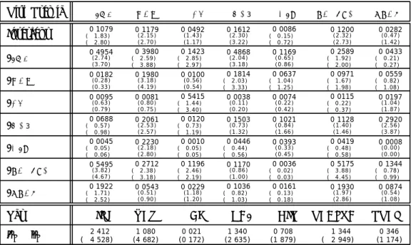
Table II reports estimates of the coefficients of the economic risk premia estimated using the minimum-variance kernel q∗t. Notice that since the instruments are demeaned, the intercept
term can be interpreted as the unconditional risk premium on ykt.
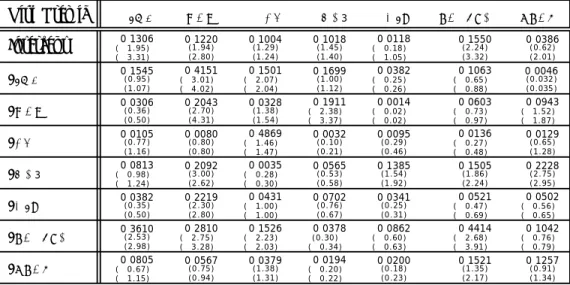
Table III reports results for the risk premia assigned by the non-negative kernel ˜qt.
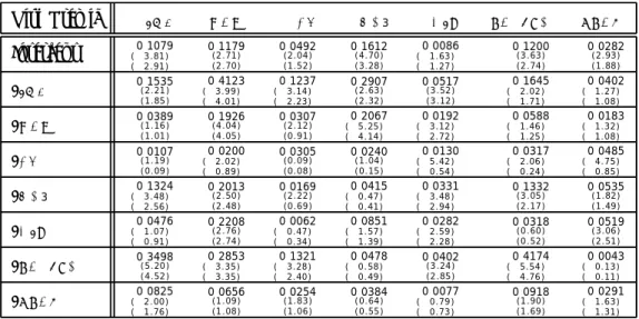
Table IV reports coefficient estimates of the economic risk premia estimated using the hedging portfolios.
The premia assigned by q∗
t and ˜qt∗ differ because the second kernel is more volatile than
the first one. The additional volatility of ˜qt may generate a correlation with the component
ofykt which is orthogonal to asset returns, and hence generate a discrepancy betweenλ∗t and
˜
λt.
The expected excess cash-flows on the hedging portfolios are identical to the risk premia assigned byq∗
t. Yet, the realized excess cash flows on the hedging portfolios in general differ
from (q∗
t −1)ykt. Hence, the estimates of the unconditional risk premia using the “q∗” and
the “hedging-portfolio” approaches will coincide, although their standard errors may differ. In addition, the impact of the conditioning variables on the conditional risk premia will also differ.
The tables report two sets of T-ratios. The first T-ratio is obtained using a two-step procedure: we first estimate the coefficients of q∗
t, ˜qt, and y∗kt. We then estimate the risk
premia by GMM. The second t-ratio is obtained estimating all parameters by GMM. The reason for the two separate approaches is that we are concerned with the large number of estimated parameters when the coefficients of the minimum-variance kernels and the hedging portfolios are estimated by GMM. As it turns out, the T-ratios change only marginally across the two procedures. In all tests, standard errors are adjusted for heteroskedasticity of unknown form and serial correlation (MA of order 11).
The results are fairly similar across the three approaches. The signs of the unconditional premia are the same, while the absolute size of the unconditional premia, as well as their significance, tend to be slightly higher when using the ˜qt approach. The patterns of time
variation, on the other hand, tend to be stronger for the risk premia assigned by qt∗ and for
In the following discussion we focus on the results from the hedging-portfolio approach, Table IV. We do this for two reasons. First, standard errors tend to be tight, and several coefficients are significant. Second, these premia correspond to actual average excess cash
flows, which are also one of the inputs to the Sharpe ratios estimated in the next exercise. The following patterns emerge from the tables:14
The unconditional inflation premium is negative, as one would expect given the nega-tive net impact of inflation on the investment-opportunity set. The premium equals -11 basis points using the q∗ and hedging portfolio approaches; it equals -13 basis points
using the ˜q approach.
There is also evidence of significant time-variation. The inflation premium is less negative for a higher real rate of interest: an increase in REALTB by one standard deviation increases the premium by 35 to 55 basis points. The premium is more negative for a steeper term structure: a one-standard deviation increase leads to an fall in the premium between.
The unconditional market risk premium is positive and significant, consistent with its positive net effect on investment opportunities.
The premium increases with stock returns, the slope of the term structure, and the dividend yield; the premium decreases with inflation and the real rate.
The unconditional consumption risk premium is positive, but insignificant. This re-sult is consistent with the somewhat weak positive effect of consumption growth on investment opportunities.
Interestingly, although the unconditional consumption risk premium is insignificant, there is significant time-variation. Namely, inflation and the real rate affect negatively the conditional consumption risk premium.
The unconditional risk premium on the slope of the term structure is positive and
14The discussion is based on the T-ratios obtained estimating the portfolio weights inside the GMM algorithm.
significant.15 This is consistent with the evidence that a steeper yield curve has a positive effect on investment opportunities.
The premium increases with the inflation rate and decreases with stock returns. The dividend-yield unconditional premium is negative and insignificant. This evidence can be reconciled with the relatively small net effect of this variable on investment opportunities.
As with the consumption premium, there is significant time-variation. The premium becomes less negative as inflation and the real rate increase. The premium becomes more negative as stock returns, the slope of the term structure, and the dividend yield increase.
The real rate of interest commands a positive unconditional risk premium. This result may appear puzzling, given the negative net effect on the risk-return trade-off. Yet, investors should care about both the slope and the position of the capital allocation line (CAL). A higher real rate of interest means an upward shift of the CAL, which may more than compensate the negative effect on the slope of the CAL.
As with other risk premia, there is significant time variation. The premium increases with the slope of the term structure and decreases with the real rate.
Finally, the default premium receives an insignificant positive unconditional risk pre-mium. This is consistent with the mildly positive net effect on investment opportuni-ties.
The premium increases with the dividend yield.
The results from the tests using industry-sorted portfolios are very similar. Based on the results above, we can draw a few conclusions:
First, the sign and significance of the unconditional risk premia associated with the selected economic variables are largely consistent with the predictability patterns previously
15It is positive, but insignificant, when estimated using the ˜q
documented. Hence, there is support for Merton’s (1973) I-CAPM intuition.
Second, conditional risk premia exhibit significant time variation. The time-varying patterns are estimated more precisely than in other studies. For example, Ferson and Harvey (1991) also document time variation in the market premium. They only find two significant effects, though: the premium increases with the dividend yield and decreases with the real rate. Our results show that two other variables affect significantly the market premium: the slope of the term structure (positive effect) and the rate of inflation (negative effect).
The risk premia estimated above coincide with the Sharpe ratios of exact hedging port-folios. But, in general, economic risk variables can be tracked only imperfectly by asset returns. Hence, in order to obtain Sharpe ratios on traded portfolios we need to standardize the estimates obtained above by the volatility of the approximate hedging portfolio cash
flows. The composition of the hedging portfolios is estimated separately from the Sharpe ratios.
Table V presents unconditional risk premia on the seven hedging portfolios, the uncondi-tional volatility on the portfolio cash-flows, and unconditional Sharpe ratios. In interpreting the results, it is useful to recall that the volatility of the portfolio cash-flows equals the square-root of the R2 coefficient of a regression of the economic variables on the asset re-turns and a constant. Hence, the Sharpe ratios are simply the products of the risk premia and the reciprocals of the square roots of the R2 coefficients.
The Sharpe ratios allow us to effectively rank the importance of the seven risk variables:
Interestingly, the largest Sharpe ratio is not associated with the market portfolio proxy, XEW, but with the term-structure variable HB3: .19 (.23 using industry-portfolio returns). The Sharpe ratio is about 20% higher than the risk premium.
The second largest Sharpe ratio is associated with the real rate of interest, REALTB,
.16, which is about 30% higher than the corresponding risk premium.
Then we have the market proxy, with .12, and consumption growth, with .09. The market proxy is tracked almost exactly by its hedging portfolio,and hence the premium
and the Sharpe ratio essentially coincide. The consumption-growth premium, on the other hand, is 91% higher than the corresponding premium.
The Sharpe ratio on the dividend yield is positive, small in absolute value, and in-significant.
The smallest Sharpe ratio, but the second largest in absolute value, is associated with the inflation rate, −.16 (52% higher, in absolute value, than the corresponding pre-mium).
We can also compare the ranking of the economic variables based on their Sharpe ratios to that based on their net effect on investment opportunities. In both rankings, HB3 is the
first variable, INF is the last one, and CG ranks fifth. The rankings of the other variables, on the other hand, are somewhat different.
The results from the industry-portfolio returns are roughly similar, although somewhat less significant.
C.
Multi-beta Models
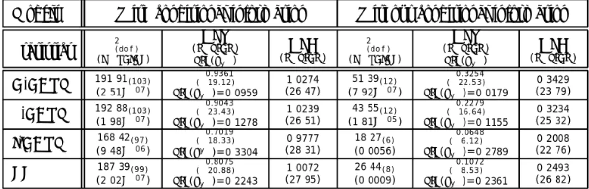
In this section we discuss the results of tests of the four multi-beta models: C-CAPM, S-CAPM, I-S-CAPM, and FF.16 Results of the tests are presented in Table VI. The tests are performed using the full set of instruments zt (“With conditional information”) and using
only the constant z1 (“Without conditional information”) to scale asset returns.
We report three statistics: i) the χ2 statistic associated with a test of the overidentifying restrictions; ii) the difference between the standard deviation of the candidate pricing kernel and the standard deviation ofq∗
t, the HJV statistic; and iii) the Hansen-Jagannathan (1997)
distance measure, the HJD statistic. We also report the p-values associated with theχ2 test, and the T-ratios associated with the HJV and HJD statistics.
16We obtained from Fama his monthly series of the size and book-to-market factors for the 1963-1993 period. We construct mimicking portfolios for the two factors using the 1963-1993 sample, and we performed the tests using the mimicking-portfolio cashflows for the full 1959-1996 period.
In the test of overidentifying restrictions, the coefficients of the candidate kernel are estimated by GMM, although the composition of the mimicking portfolios is estimated sep-arately, outside of the GMM algorithm. This is because we wanted to ensure that the coefficients of the mimicking portfolios exactly satisfied the orthogonality conditions (51)-(52). The shortcoming of this approach is that the size of the test is not adjusted for the sampling variability in the estimates of the hedging-portfolio weights, and hence the test tends to reject too often.
In the tests based on the HJV and HJD, the coefficients of the candidate kernel are estimated separately from the statistics themselves. This means that the test take the form of the candidate kernel asgiven.
Overall, the table shows that while all four models are formally rejected, in both con-ditional and unconcon-ditional tests, their performance varies considerably. Across tests, the I-CAPM is the best performer, followed by the FF model, the S-CAPM, and the C-CAPM. In most tests, though, the difference in performance between the C-CAPM and the S-CAPM is modest. Comparing conditional and unconditional tests, the conditional tests tend to de-emphasize the differences across models and to lead to stronger rejections that the un-conditional tests.
We now turn to a discussion of the different tests. We begin with the conditional tests. The χ2 tests strongly reject all four models. Interestingly, the χ2 statistics are very similar for the C-CAPM and the S-CAPM, 191.91 and 192.88, respectively. The FF model has only a slightly lower χ2 statistic, 187.39, whereas the I-CAPM has the lowest statistic, 168.42, although the rejection is still very strong. Hence, the performance of the four models is remarkably similar. One way to understand this feature is to note the total number of scaled returns that the restricted MV kernel must price is very large relative to the number of factors: we have N = 13 and J = 8, for a total of 104 scaled returns, while the number of factors ranges from 1 (C-CAPM and S-CAPM) to 5 (FF) and 7 (I-CAPM). Hence, the addition of even 6 factors makes little difference when the total number of securities to price is so large.
The HJV tests also strongly reject all four models. For a better understanding of the economic magnitudes involved, it is worth noting that the standard deviation of the MV kernel constructed using the original scaled returns is 1.033. The standard deviations of the restricted MV kernels implied by the C-CAPM and S-CAPM are one order of magnitude
smaller, 0.0959 and 0.1278, respectively. The restricted MV kernel implied by the FF model has a standard deviation of 0.2243, whereas the MV kernel of the I-CAPM kernel has a standard deviation of 0.3304. Hence, the comparison of standard deviations allows to better differentiate the four models. In particular, the increase in volatility going from the FF model to the I-CAPM amounts to more than 47%.
The HJD tests deliver essentially the same message as the comparison of standard devi-ations. While the highest HJD statistic is for the C-CAPM, 1.0274, the S-CAPM delivers a very similar result, 1.0239. The FF model leads to a statistic not very dissimilar, 1.0072. The lowest HJD statistics is for the I-CAPM, 0.9777.
We now turn to the unconditional tests.
The χ2 statistic now favors the S-CAPM relative to the C-CAPM: 43.55 vs 51.39. The statistic for the FF model is substantially lower, 26.44. The I-CAPM performs best, with a statistic of 18.27. The p-values of the statistics are overall much higher than in the conditional tests, the highest being for the I-CAPM model, 0.56%. Hence, in unconditional tests, the
χ2 statistics better differentiate across models, with the I-CAPM being markedly the best performer.
In interpreting the HJV tests it is worth noting that the standard deviation of the MV kernel constructed using the original returns is 0.3438. In comparison, the standard deviation of the MV kernel restricted by the C-CAPM is very low, 0.0179. Considerably higher is the standard deviation of the S-CAPM, 0.115. Further increases in volatility are obtained by the FF model, 0.2361, and especially by the I-CAPM, 0.2789. Hence, we have again a marked variation in performance across models, with the I-CAPM being by far the bet performer.
Finally, we examine the results of HJD tests. The statistics for the C-CAPM and S-CAPM are fairly similar, 0.3429 and 0.3234, respectively. Substantially lower are the
statis-tics for the FF model, 0.2493, and for the C-CAPM model, 0.2008.
While not reported in the table, we also performed the tests using industry-sorted stock portfolios. As in the other tests, using industry-sorted portfolio returns introduces more noise in the estimation. This translates into less precise estimates and, in this case, in somewhat less dramatic rejections of the multi-beta models.
VI.
Conclusions
This paper presents a new approach for the estimation of risk premia associated with ob-servable sources of risk, which is based on the moments of the minimum-variance kernel of Hansen and Jagannathan (1991). Consistent with the I-CAPM intuition, we find that vari-ables that significantly affect the position of the investment-opportunity set (the conditional means and volatilities of asset returns) also tend to receive non-zero risk premia. More-over, variables that positively (negatively) affect the Sharpe ratio tend to receive positive (negative) risk premia.
We also provide extensive evidence on the performance of explicit asset-pricing models: the C-CAPM, the S-CAPM, the I-CAPM, and the FF model. While all models are formally rejected, the FF model and the I-CAPM perform substantially better than the static CAPM and the consumption CAPM. In addition, wefind that the I-CAPM consistently outperforms the FF model.
References
[1] Balduzzi, Pierluigi, and H`edi Kallal, 1997, Risk premia and variance bounds, Journal of Finance 52, 1913-1949.
[2] Breeden, Douglas T., 1979, An intertemporal asset pricing model with stochastic con-sumption and investment opportunities, Journal of Financial Economics 7, 265-296. [3] Breeden, Douglas T., Michael R. Gibbons, and Robert H. Litzenberger, 1989, Empirical
tests of the consumption-oriented CAPM, Journal of Finance 44, 231-262.
[4] Burmeister, Edwin, and Marjorie B. McElroy, 1988, Joint estimation of factor sensitiv-ities and risk premia for the arbitrage pricing theory, Journal of Finance 43, 721-733. [5] Cecchetti, Stephen G., Pok-Sang Lam, and Nelson C. Mark, 1994, Testing volatility
restrictions on intertemporal marginal rates of substitution implied by Euler equations and asset returns, Journal of Finance 49, 123-152.
[6] Chan, Louis K. C., Jason Karceski, and Josef Lakonishok, 1998, The risk and return from factors, Journal of Financial and Quantitative Analysis 33, 159-188.
[7] Chen, Nai-Fu, Richard Roll, and Stephen A. Ross, 1986, Economic forces and the stock market, Journal of Business59, 383-403.
[8] Cochrane, John, and Lars P. Hansen, 1992, Asset pricing explorations for macroeco-nomics, NBER Macroeconomics Annual.
[9] Cochrane, John, and Jesus Sa´a-Requejo, 2000, Beyond arbitrage: good deal asset price bounds in incomplete markets, Journal of Political Economy108, 79-119.
[10] DeRoon, Frans A., and Theo E. Nijman, 2001, Testing for mean-variance spanning: a survey, Journal of Empirical Finance 8, 111-155.
[11] Downs, David H., and Karl N. Snow, 1994, Sufficient conditioning information in dy-namic asset pricing, Working Paper, University of North Carolina.
[12] Dumas, Bernard, and Bruno Solnik, 1995, The world price of foreign exchange risk,
Journal of Finance 50, 445-479.
[13] Fama, Eugene F., and Kenneth R. French, 1993, Common risk factors in the returns on stocks and bonds, Journal of Financial Economics33, 3-56.
[14] Ferson, Wayne E., and Campbell R. Harvey, 1991, The variation of economic risk pre-miums, Journal of Political Economy99, 385-415.
[15] Ferson, Wayne E., and Campbell R. Harvey, 1999, Conditioning variables and the cross-section of stock returns, Journal of Finance 54, 1325-1360.
[16] Hansen, Lars P., and Ravi Jagannathan, 1991, Implications of security market data for models of dynamic economies, Journal of Political Economy 99, 225-262.
[17] Hansen, Lars P., and Ravi Jagannathan, 1997, Assessing specification errors in stochas-tic discount factors models, Journal of Finance52, 557-590.
[18] Hansen, Lars P., and Scott F. Richard, 1987, The role of conditioning information in deducing testable restrictions implied by dynamic asset pricing models, Econometrica
55, 587-613.
[19] Hansen, Lars P., and Kenneth J. Singleton, 1982, Generalized instrumental variables estimation of nonlinear rational expectations models, Econometrica 50, 1269-1286. [20] Jagannathan Ravi, and Zhenyu Wang, 2001, Efficiency of the stochastic discount factor
method for estimating risk premiums, Unpublished Manuscript, Northwestern Univer-sity and Columbia UniverUniver-sity.
[21] Kirby, Chris, 1998, The restrictions on predictability implied by rational asset pricing models, Review of Financial Studies 11, 343-382.
[22] Lamont, Owen, 2001, Economic Tracking Portfolios, forthcomingJournal of Economet-rics.
[23] McElroy, Marjorie, and Edwin Burmeister, 1988, Arbitrage pricing theory as a restricted nonlinear multivariate regression model: ITNLSUR estimates, Journal of Business and Economic Statistics 6, 29-42.
[24] Merton, Robert, 1973, An intertemporal capital asset pricing model, Econometrica 41, 867-887.
Table I
Predictability and Heteroskedasticity
We report estimates of a predictive model of the conditional mean and volatility of the returns on ten size-sorted equity portfolios,r1. . . r10, and on three bond portfolios,rT B6,rCORP, andrGOV. Both conditional mean and conditional volatility are assumed to be linear linear functions of the lagged economic variables. INF denotes the monthly rate of inflation (percentage points per month). XEW is the equally-weighted NYSE-AMEX-NASDAQ index return less the monthly inflation rate (percentage points per month). CG is the monthly growth rate of per-capita real consumption of nondurables and services (percentage points per month). HB3 is the 1-month return of a 3-month Treasury bill less the 1-month T-bill rate (percentage points per month). DIV is the monthly dividend yield on the Standard and Poor’s 500 stock index (percentage points per month). REALTB is the real 1-month Treasury bill rate (percentage points per month). PREM represents the yield spread between Baa and Aaa rated bonds (percentage points per month). T-statistics, in parentheses, are adjusted for heteroskedasticity and serial correlation. The sample period is 1959:3-1996:11.
Panel A: Slope Estimates of Mean Equations
Var INF XEW CG HB3 DIV REALTB PREM
r1 (−−23..148219) 2.328 (6.111) 0.074 (0.992) 1.057 (2.164) 1.277 (2.324) − 1.104 (−1.959) 0.251 (0.601) r2 (−−23..491918) (51..905867) (−−00..005077) (21..026144) (21..448935) <