What most Matters in Strengthening Educational Competitiveness?: An Application of FS/QCA Method

(1)

Procedia - Social and Behavioral Sciences 197 ( 2015 ) 2182 – 2190

Peer-review under responsibility of Academic World Education and Research Center. doi: 10.1016/j.sbspro.2015.07.354

ScienceDirect

7th World Conference on Educational Sciences, (WCES-2015), 05-07 February 2015, Novotel

Athens Convention Center, Athens, Greece

What most matters in strengthening educational competitiveness?:

An Application of FS/QCA method

Young-Chool Choi

a

*, Ji-Hye Lee

b a_{Chungbuk National University, Cheongju City, Korea}

b_{Seowon University, Cheongju City, Korea}

Abstract

This study was conducted in order to investigate the relationships between different factors affecting educational competitiveness, which is crucial to enhancing national competitiveness in every country, and to put forward policy implications whereby each country may raise the level of its educational competitiveness. PISA score was selected as an indicator representing the educational competitiveness of 22 OECD countries, and this included some independent variables, such as per capita GDP, total public expenditure on education as a percentage of GDP, and total per capita public expenditure on education (US dollars), affecting educational competitiveness. We employed the fuzzy set analysis method (FS/QCA) to analyze the complex causal relationships among the factors affecting educational competitiveness. The research results show that there are three significant combinations of variables affecting educational competitiveness (PISA score). Model 1 is a configuration of four variables (high total expenditure on education as a percentage of GDP, high total per capita expenditure on education, high ratio of private-source expenditure on education to GDP, and high GDP), and includes Netherlands, Finland, Australia, and Ireland. Model 2 is a configuration of five variables (low total expenditure on education, low total per capita expenditure on education, low ration of students to teaching staff, low private-source expenditure on education, and low GDP, and includes Poland. Model 3 is a configuration of five variables (low total expenditure on education, low total per capita expenditure on education, high private-source expenditure on education, high ratio of students to teaching staff, and high GDP), and includes Japan. Finally, the study suggests that each country should endeavour to enhance its own educational competitiveness, considering how the factors associated with this relate to each other.

Peer-review under responsibility of Academic World Education and Research Center.

* Young-Chool Choi. Tel.: +82432612203; fax: +82432711137.

E-mail address: [email protected]

(2)

Keywords: educational competitiveness, FSQCA, Qualitative Comparative Analysis, education policy

1. Introduction

It is generally accepted that educational competitiveness can greatly affect national competitiveness. International institutions such as the International Institute of Management and Development (IMD) and the World Economic Forum (WEF) have published reports on the national competitiveness of different countries. Educational

competitiveness, as a sub-branch of national competitiveness, is regarded as an important element in national

development. Hence, researchers and practitioners have primarily concentrated on which factors are most strongly associated with enhancing educational competitiveness, and on how to strengthen it. However, most studies have tended to select educational infra, including the percentage of secondary student enrollments among persons of the same age or the percentage of illiterate persons among people over fifteen years of age, as a dependent variable representing educational competitiveness. However, although factors connected with educational infra can be components of educational competitiveness, they are not suited to representing the final variable which educational

competitiveness is oriented towards. With this background in mind, this study selects international educational

achievement score as a final dependent variable to denote educational competitiveness, which is understood as a tool for evaluating the learning achievements of students and how these change over time. The main reason for selecting

the variable educational competitiveness as a dependent variable is that most countries in the world are now trying

to strengthen their educational competitiveness and the quality of the education they provide on the basis of their international educational achievement score, which they are also using as objective evidence in their attempts to ameliorate their educational environment (KEDI, 2010). The international institutions which evaluate students’ achievements from a comparative perspective are the International Association for the Evaluation of Educational

Achievement (IEA) and the OECD. The former publishes Trends in International Mathematics and Science Study

(TIMSS), while the latter publishes the reports of the Programme for International Student Assessment (PISA). TIMSS and PISA are concerned with evaluating students’ achievements in, respectively, mathematics and science, and reading, mathematics, and science. This study selects PISA score as a final indicator to represent educational competitiveness. PISA, as mentioned above, is organized by the OECD, and assesses the extent to which 15-year-old students have acquired key knowledges and skills that are essential for full participation in modern society. It is assumed that PISA score differences between countries are attributable to differences in administrative and financial infras. However, empirical studies in these areas have so far been limited. With this background in mind, this study attempts to identify factors associated with educational competitiveness, to investigate which factor is most strongly related to it, and to analyze how these factors may be causally interrelated, using the structural equation modeling approach. Through this study, scholars and policy practitioners involved in educational policy are expected to understand the factors affecting educational competitiveness and to utilize them in order to enhance the quality of education at central and local levels.

2.Theoretical background

2.1.Educational competitiveness

It is assumed that the term ‘competitiveness’ is derived from the term ‘national competitiveness’, or ‘regional competitiveness’. International institutions such as the International Institute of Management Development (IMD) and the World Economic Forum (WEF) have used the term ‘national competitiveness’ or ‘global competitiveness’.

The IMD publishes the World Competitiveness Yearbook, while the WEF publishes its Global Competitiveness

Report annually. These bodies define the term ‘national competitiveness’ as the ability of a nation to create and maintain an environment that sustains greater value creation in its enterprises and more prosperity for its people (IMD, 2013: 480–1); however, the term is sometimes defined differently. The IMD and WEF categorize the field of national competitiveness into a dozen sub-categories, with education normally being contained in the sub-category

infra. Consonant with the definition of the term ‘competitiveness’, educational competitiveness can be defined as the ability of a nation to create and maintain an environment which sustains quality of education and greater

(3)

prosperity for its people. This definition can cause some confusion or differences of opinion among scholars. However, on the assumption that any area of national competitiveness has to make contributions toward enhancing the quality of life of ordinary people and making their lives more comfortable, it would be possible for us to define ‘educational competitiveness’ in the same way as the term ‘national competitiveness’ is defined. What, then, are the

components of educational competitiveness? WEF’s Global Competitiveness Report classifies national

competitiveness into 12 pillars. Of these, pillar 4 is made up of factors relating to primary education and pillar 5 of factors relating to higher education. In this paper, educational competitiveness includes primary education and secondary education and excludes higher education, and so it is more related to the indicators contained in pillar 4. In order to measure educational competitiveness, we can use composite indicators or a single indicator, and either quantitative or qualitative indicators. In this regard, the IMD uses 15 composite plural indicators, including hard and soft education data, to measure educational competitiveness. This is different from the method the WEF uses, in that the WEF distinguishes primary- and secondary-education-related indicators from higher-education-related indicators. Today, primary and secondary education is believed to foster innovation and creativity, which are crucial for strengthening national competitiveness. In other words, if a country’s primary and secondary education is not competitive, this can prove an obstacle to the innovativeness of that country, weakening its growth potential and the creativity of its young people (WEF, 2013: 5). As regards the contribution of educational competitiveness to national competitiveness, primary and secondary education is more important than higher education. Therefore, in this study, we focus on primary and secondary education, rather than on higher education, in dealing with educational competitiveness.

The next important factor is which indicators can be included in the indicator set for constructing national competitiveness. Indicators can be composite or single, or hard data or soft data. Here, seeing that we focus primarily on primary and secondary education, and that we also believe that creativity and innovation in terms of national human resources are highly important for national development, we adopt PISA score as a representative indicator for educational competitiveness. In this study, the PISA score published in 2013 by the OECD is used. PISA evaluates the extent to which 15-year-old students have acquired mathematics, science and reading skills, which are essential for their successful activity in society. PISA results reveal what is possible in the field of education, by showing what students in the highest-performing and most rapidly improving education system can do (OECD, 2013: 3). It is hypothesized that the higher the PISA score, the stronger will be educational competitiveness.

2.2.Factors affecting educational competitiveness

It is generally understood that many factors can affect the educational competitiveness of a country, and many studies have indicated that a number of factors can be involved in improving the educational sector in one country. Here, we address the potential factors associated with educational competitiveness and their interrelationships.

First, we hypothesize that per capita GDP is associated with total expenditure on education. In OECD member countries, the proportion of total expenditure on education as a percentage of GDP is relatively high, accounting for approximately 5.6 percent of GDP in 2006. The proportion of expenditure on primary and secondary education is 3.7 percent of GDP, whereas that of expenditure on higher education is 1.4 percent of GDP (OECD, 2010). The expenditure of OECD member countries on education increased by 28 percent between 2000 and 2006, reaching an average annual growth rate of 4 percent. In spite of the fact that expenditure on education nowadays accounts for a large proportion of GDP, and also has been increasing constantly, there have been few studies proving that growth in education spending leads to growth in educational quality. In the meantime, some studies (Choi, 2008; Shin and Joo, 2013) have concluded that accumulated per capita expenditure on education has positively affected PISA score. On the basis of these research findings, this study hypothesizes that per capita GDP, total expenditure on education, and total per capita expenditure on education affect educational competitiveness, and that per capita GDP also affects total expenditure on education as a percentage of GDP, and total per capita expenditure on education.

(4)

Second, we hypothesize that parents’ concerns about education is associated with educational competitiveness. It is important, in relation to educational competitiveness, whether parents are strongly concerned about a student’s future career or not. This is more important in Asian than in Western societies. Parental concerns about children’s education can be represented by total expenditure on education burdened by the private sector. There have been few studies examining the relationships between total expenditure on education burdened by the private sector and educational competitiveness. Here, following the work of some scholars (Choi, 2008; KEDI, 2010), we hypothesize that private-source expenditure on education as a percentage of GDP is positively associated with educational competitiveness.

Third, we hypothesize that pupil–teacher ratio can affect educational competitiveness. The ratio of students to teaching staff is an important issue as regards the quality of education worldwide. It is assumed that the smaller the number of students a teacher can teach, the greater will be the effectiveness of the teaching.

In summary, we include per capita GDP, total expenditure on education as a percentage of GDP, total per capita expenditure on education, ratio of students to teaching staff, and parents’ concerns about education as independent variables affecting the dependent variable, educational competitiveness.

2.3.Research questions

On the basis of the theoretical discussion above, we suggest the following two research questions: Which configurations can affect educational competitiveness as a dependent variable?

3. Research design

3.1.Variables

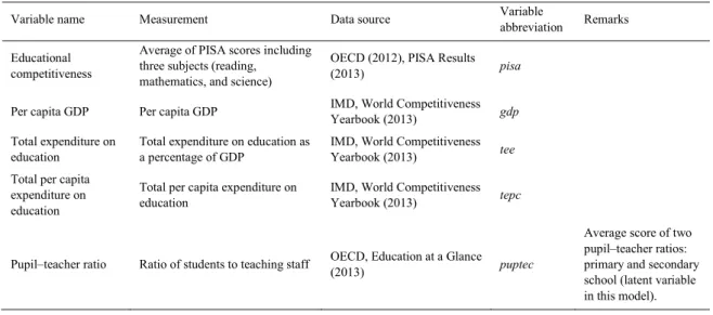
The countries to be included in this analysis are OECD member countries. Among 34 OECD countries, twelve countries including Mexico and New Zealand, are excluded because of problems with data. The variables analyzed in this research consist of five independent variables and one dependent variable. The five independent variables are: per capita GDP, total expenditure on education as a percentage of GDP, total per capita expenditure on education, ratio of students to teaching staff, and parental concerns about children’s education. The one final dependent variable is educational competitiveness. Table 1 explains the names of the variables, their measurement, and their data source.

Table 1 Variables and data source

Variable name Measurement Data source Variable _abbreviation Remarks

Educational competitiveness

Average of PISA scores including three subjects (reading,

mathematics, and science)

OECD (2012), PISA Results (2013) pisa

Per capita GDP Per capita GDP IMD, World Competitiveness _{Yearbook (2013)} gdp

Total expenditure on education

Total expenditure on education as a percentage of GDP

IMD, World Competitiveness Yearbook (2013) tee Total per capita

expenditure on education

Total per capita expenditure on education

IMD, World Competitiveness Yearbook (2013) tepc

Pupil–teacher ratio Ratio of students to teaching staff OECD, Education at a Glance (2013) puptec

Average score of two pupil–teacher ratios: primary and secondary school (latent variable in this model).

(5)

Parental concerns about children’s education

Ratio of private-source expenditure on education to GDP

OECD, Education at a Glance

(2013) privat exp

3.2.Analysis method

As the data used in this study include 22 cases, conventional quantitative methods are difficult to apply in such a small N research design. QCA, however, offers an alternative approach to investigating the research question of this study. QCA is a case-oriented analytic technique that can systematically deal with small number of cases (i.e. 5-50) by applying “Boolean algebra to implement principles of comparison used by scholars engaged in the qualitative study of macro social phenomena (Zeng, 2013: 230-231). It is proposed by Ragin (1987) and has gradually developed into a widely applied method in various research fields. In the field of public administration, there are not many studies using QCA. As the outcome can be produced by multiple causal mechanisms, one feature of QCA is that it considers the outcome a result of the combination of several conditions. Differently from the regression analysis which can only tell the relationships among independent variables affecting dependent variable, QCA can detect conditioning effects of independent variables and specify paths to the outcome. The first state in a QCA, like other methods is to show descriptive statistics of the variables included in the analysis. Then, it is necessary to standardize the original values of each variable in order to address the problems relating to mean and standard deviation of each variable occurring in the analysis process. The next stage is to produce fuzzy set membership score of each variable. For this, we used the fs/QCA calibrate function. This function requires three values of the variable as anchor points that indicate (1) full membership in the set; (2) full non membership in the set; ant (3) the point of maximum ambiguity (neither in nor out of the set) (Ragin, 2010). Conventionally, a membership of 0.95 or

greater indicates an item that is Āfully or nearly fully inā the set; a membership of 0.05 or less indicates an item

that is Āfully out or nearly fully outā of the set; and a membership of 0.5 indicates the point of maximum of

ambiguity as to membership in the set (Thygeson, et al. 2011: 25-26). And then, the next step is to build a truth table with data for selected cases regarding the causal conditions and the outcome variables. Truth tables list the logically possible combinations of conditions and the outcome associated with each combination (Poveda, 2013). Next, investigation of a truth table by itself allows for a study of diversity, showing which configurations are common and which ones do not happen or happen very seldom. Finally, we produce configuration explaining educational competitiveness.

4. Research results

4.1.Descriptive statistics

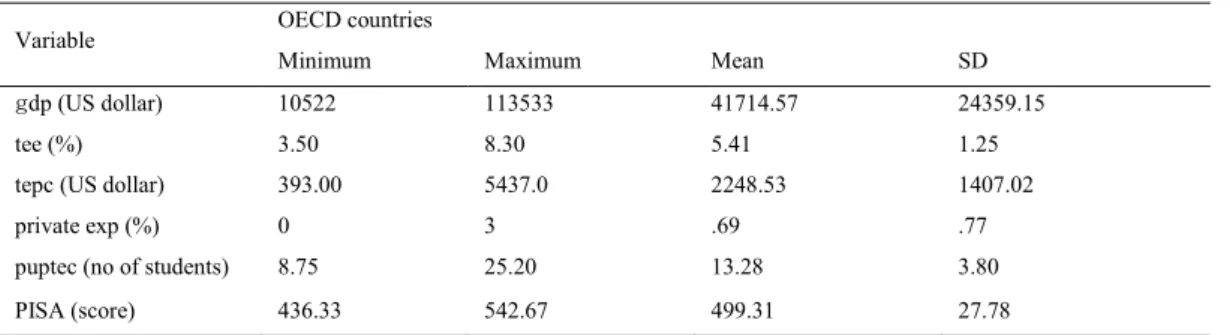
Table 2 presents descriptive statistics for the constructs analyzed in our study, including means, standard deviations, and the minimum and maximum of the variables contained in the final sample of 22 OECD countries.

Table 2 Descriptive statistics Variable OECD countries

Minimum Maximum Mean SD

dp (US dollar) 10522 113533 41714.57 24359.15 tee (%) 3.50 8.30 5.41 1.25 tepc (US dollar) 393.00 5437.0 2248.53 1407.02 private exp (%) 0 3 .69 .77 puptec (no of students) 8.75 25.20 13.28 3.80 PISA (score) 436.33 542.67 499.31 27.78

(6)

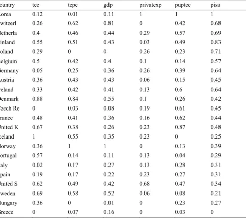
Table 3 shows fuzzy set membership scores of variables included in the analysis, which were converted by the “calibrate” procedure using Fs/QCA program.

Table 3 Fuzzy set membership score of variables by county

country tee tepc gdp privatexp puptec pisa Korea 0.12 0.01 0.11 1 1 1 Switzerl 0.26 0.62 0.81 0 0.42 0.68 Netherla 0.4 0.46 0.44 0.29 0.57 0.69 Finland 0.55 0.51 0.43 0.03 0.49 0.83 Poland 0.29 0 0 0.26 0.23 0.71 Belgium 0.5 0.42 0.4 0.1 0.14 0.57 Germany 0.05 0.25 0.36 0.26 0.39 0.64 Austria 0.36 0.43 0.43 0.06 0.15 0.45 Ireland 0.33 0.42 0.41 0.13 0.6 0.64 Denmark 0.88 0.84 0.55 0.1 0.26 0.42 Czech Re 0 0.03 0.08 0.19 0.61 0.45 France 0.48 0.41 0.36 0.16 0.62 0.44 United K 0.67 0.38 0.26 0.23 0.87 0.48 Iceland 1 0.55 0.35 0.23 0 0.25 Norway 0.36 1 1 0 0.13 0.39 Portugal 0.57 0.14 0.11 0.13 0.04 0.29 Italy 0.02 0.17 0.27 0.13 0.28 0.31 Spain 0.19 0.17 0.22 0.23 0.27 0.31 United S 0.62 0.49 0.42 0.68 0.47 0.34 Sweden 0.69 0.58 0.52 0.06 0.08 0.21 Hungary 0.36 0 0.01 0 0.23 0.27 Greece 0 0.07 0.16 0 0.03 0

4.2.Truth table analysis

Table 4 shows the result of the truth table analysis. Here what should be done is to distinguish configurations that are subsets of the outcome from those that are not. Values below 0.75 indicate substantial inconsistency. The 1s and 0s indicated the different corners of the vector space defined by the fuzzy set causal conditions. It is now necessary to indicate which configurations can be considered subsets of the outcome and which cannot. In this Table 4, there are three configurations (solutions) which meet the consistency level.

Table 4 Truth table

tee tepc privatexp puptec gdp number pisa raw consist.

0 0 1 0 0 1 1 1 0 0 1 1 1 1 1 1 1 1 0 1 1 3 1 1 1 1 1 1 1 4 1 0.75 0 0 0 0 0 2 0 0.5 0 0 1 0 1 2 0 0.5 0 0 1 1 0 2 0 0.5 0 1 0 0 1 2 0 0.5 1 1 0 0 1 5 0 0.4 0 0 0 1 0 3 0 0.333333 0 0 0 0 1 1 0 0 1 0 1 1 0 1 0 0

(7)

1 1 1 0 1 1 0 0

1 0 0 0 0 2 0 0

Note: number means the number of cases with greater than 0.5n membership in that corner of the vector space and raw consist

means the degree to which membership in that corner of the vector space is a consistent subset of membership in the outcome.

Figure 1 shows the output for the most parsimonious solution for the educational competitiveness. Here, 0.75 was

given as the consistency cutoff. The solution indicates three paths to educational competitiveness.

Figure1. Truth table analysis

G Dojrulwkp=#Txlqh0PfFoxvnh|G Wuxh=#4# G G G G G G 000#WUXWK#WDEOH#VROXWLRQ#000G G G G G G iuhtxhqf|#fxwrii=#41333333G G G G G G frqvlvwhqf|#fxwrii=#31:83333G G G G G G Dvvxpswlrqv=G G G G G G G G udzG fryhudjhG xqltxh#G fryhudjhG frqvlvwhqf|G G G G 00000000000G 00000000000G 00000000000G G whh䔡whsf䔡sxswhf䔡jgsG G G G G G whh䔡 whsf䔡 sulydwh{s䔡 sxswhf䔡 jgsG G G G G G whh䔡 whsf䔡 sulydwh{s䔡 sxswhf䔡 jgsG G G G G G vroxwlrq#fryhudjh=#G G G G G G vroxwlrq#frqvlvwhqf|=#G G G G G G Fdvhv#zlwk#juhdwhu#wkdq#318#phpehuvkls#lq#whup#whh䔡whsf䔡sxswhf䔡jgs=#Qhwkhuodqgv4,#+4/4,#/G Ilqodqg#+4/4,#/#Dxvwudold#+4/4,#/#Luhodqg#+4/4,#/G Iudqfh#+4/4,#/#Xqlwhg#Nlqjgrp#+4/4,#/#Xqlwhg#Vwdwhv#+4/3,G

Fdvhv#zlwk#juhdwhu#wkdq#318#phpehuvkls#lq#whup#whh䔡whsf䔡sulydwh{s䔡sxswhf䔡jgs=#Srodqg#+4/4,G

Fdvhv#zlwk#juhdwhu#wkdq#318#phpehuvkls#lq#whup#whh䔡whsf䔡sulydwh{s䔡sxswhf䔡jgs=#Mdsdq#+4/4,G

Figure 1 above includes measures of coverage and consistency for each solution term and for the solution as a whole. As shown in the Table, the solution coverage of the completed solution is 0.5333, whereas the solution

consistency of it is 0.88, which are statistically acceptable. Consistency measures the degree to which solution terms

and the solution as a whole are subsets of the outcome. Unique coverage measures the proportion of membership in

the outcome explained solely be each individual solution term. Raw coverage measures the proportion of

membership in the outcome explained by each term of the solution. Solution coverage measures the proportion of

membership in the outcome that is explained by the complete solution. Solution consistency measures the degree to

which membership in the solution is a subset of membership in the outcome. With Fs/QCA, the consistency of the set-theoretical relationship is analogous to the p-value. Consistency greater than 0.90 indicates a strong, empirical significant relationship, much as a p-value less than 0.05 indicates a low probability that the findings in a conventional statistical analysis are a chance observation (Thygeson et al., 2011:39).

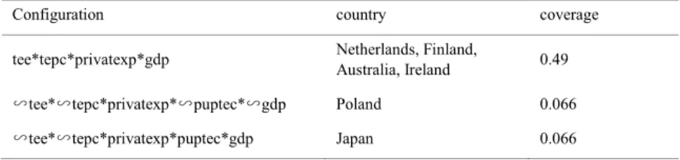
The findings of the Fs/QCA show there are three configurations explaining educational competitiveness of OECD countries. Table 5 below summarizes them.

(8)

Table 5 Analysis result

Configuration country coverage tee*tepc*privatexp*gdp Netherlands, Finland, _{Australia, Ireland} 0.49

ītee*ītepc*privatexp*īpuptec*īgdp Poland 0.066

ītee*ītepc*privatexp*puptec*gdp Japan 0.066 Note: ଭmeans Logical Not

As shown in Table 5, there are three configurations explaining educational competitiveness in OECD countries. Model 1 is a configuration of four variables (high total expenditure on education as a percentage of GDP, high total per capita expenditure on education, high ration of private-source expenditure on education to GDP, and high GDP), and includes Netherlands, Finland, Australia, and Ireland. Model 2 is a configuration of five variables (low total expenditure on education, low total per capita expenditure on education, low ration of students to teaching staff, low private-source expenditure on education, and low GDP, and includes Poland. Model 3 is a configuration of five variables (low total expenditure on education, low total per capita expenditure on education, high private-source expenditure on education, high ratio of students to teaching staff, and high GDP), and includes Japan.

5. Conclusion

The main purpose of this study is to demonstrate specific configuration models explaining educational competitiveness in OECD countries, in order both to portray the causal connections between GDP, total expenditure on education as a percentage of GDP, total per capita expenditure on education, private-source expenditure on education as a percentage of GDP, ratio of students to teaching staff as independent variables and educational competitiveness as a dependent variable, and to put forward policy implications whereby each country can strengthen its educational competitiveness. Following the requirements of the FS/QCA model specification, we converted actual value of each variable to fuzzy set membership scores, produced truth table, and derived the three

configurations explaining educational competitiveness. The three configurations are: tee*tepc*privatexp*gdp, ī

tee*ītepc*privatexp*īpuptec*īgdp, and ītee*ītepc*privatexp*puptec*gdp.

FS/QCA is an alternative approach to analysis in educational competitiveness that involves truth tables, Boolean algebra and search for a greater understanding of causal conditions. The use of QCA has been rarely reported in educational competitiveness studies, and is likely to be conceptual and paradigmatic challenges to its adoption in some settings. The potential of FS/QCA to refocus research questions and to offer a logical interpretation of combinations of qualitative and quantitative data may be especially useful for many small cases studies.

Some limitations of this study can be identified. First, it is important to remember that this study has focused primarily on OECD member countries. Even though this research result supports the constructed hypotheses, it could result in a narrow view of the effects of educational competitiveness effects, one that it might not be possible to extrapolate to other country groups less sensitive to the influence of economic and financial factors. Second, many variables exist which could influence the variables considered in the study, but which are not present in the study’s conceptual model. More interesting and valid conclusions could be drawn from a more global study that could consider non-economic and non-financial factors, such as organizational structure and adequacy of teaching method.

Acknowledgements

This work was supported by the National Research Foundation of Korea Grant funded by the Korean Government (NRF-2012-413-B0031)

(9)

References

Adam, A., Delis, M., Kammas, P. (2008). Fiscal decentralization and public sector efficiency: evidence from OECD countries. CESIFA working paper no. 2364.

Biever, T. and Martens, K. (2011). The OECD PISA study as a soft power in education? Lessons from Switzerland and US, European Journal of Education, 46(1), part 1.

Borgonovi, F., Montt, G. (2012). Parental involvement in selected PISA countries and economies. OECD Education working paper no. 73. Cakar, F. and Karatas, Z. (2012). The self-esteem, perceived social support and hopelessness in adolescents: the structural equation modeling,

Educational Sciences: Theory and Practice 12(4), 2406–12.

Chien, H., Kao, C., Yeh, I. and Lin, K. (2012). Examining the relationship between teachers’ attitudes and motivation toward web-based professional development: a structural equation modeling approach, TOJET, 11(2), 120–7.

Choi, Y. C. (2008). Relationships between national competitiveness and decentralization, Korean Association of Local Government Studies Summer Conference Proceedings.

Enikolopov, R., Zhuravskaya, E. (2007). Decentralization and political institutions, Journal of Public Economics, 91, 2261–90. Fisman, R., Gatti, R., (2002). Decentralization and corruption: evidence across countries, Journal of Public Economics 83, 325–46.

Gao, S., Mokhtarian, P. and Johnston, R. (2008). Exploring the connections among job accessibility, employment, income, and auto ownership using structural equation modeling, Ann Reg Sci, 42, 341–56.

Hayduck, L. A. (1987) Structural Equation Modeling with LISREL: Essentials and advances. Baltimore, MD: Johns Hopkins.

Holzinger, K. and Knill, C. (2008). Theoretical framework: causal factors and convergence expectations, in K. Holzinger, C. Knill and B. Arts (eds), Environmental Policy Convergence in Europe: The impact of international institutions and trade. Cambridge: Cambridge University Press.

Huh, J. (2013). Advanced Structural Equation Modeling by AMOS. Seoul: Hanare Academy. IMD (2013). World Competitiveness Yearbook. Geneva: IMD.

KEDI (2010). Analysis of Effects of Education on National Competitiveness. Seoul: KEDI. KICE (Korea Institute for Curriculum and Evaluation). Homepage.

Laglera, J. M., Collado, J. and Oca, J. A. M. (2013). Effects of leadership on engineers: a structural equation model, Engineering Management Journal, 25(4), 7–16.

Lee, C. and Lee, K. H. (2006). Analysis of the Conditions of Korea Education Competiveness Index of IMD World Competitiveness Yearbook.

The Journal of Korean Education, 33(1), 173-197.

Lingard, B. and Grek, S. (2007). The OECD, indicators and PISA: an exploration of events and theoretical perspectives. Edinburgh, ESRC/ESP Research Project.

OECD (2010). Education at a Glance. Paris: OECD. OECD (2013). PISA 2012 Results in Focus. Paris: OECD.

Ragin, C. (2000). Fuzzy-Set Social Science. Chicago: The University of Chicago Press.

Rowan, Correnti, and Miller (2002). What large scale,survey research tells us about teacher effects on student achievement: insight from the “prospect” study of elementary schools. CPRE research report series.

Shin, H. S. and Joo, Y. H. (2013). Global governance and educational policy in Korea, Korean Journal of Educational Research, 51(3), 133–59. Tanzi, V. and Schuknecht, L. (1998). Can small governments secure economic and social well being?, in Grubel, H. (ed.), How To Spend the

Fiscal Dividend: What is the optimal size of government? Vancouver: Fraser Institute.

Thygeson, M.M., Solberg, L., Asche, S.E., Fontaine, P., Pawlson, L. G., Scholle, S.H. (2011). Using Fuzzy Set Qualitative Comparative Analysis to Explore the Relationship between Medical Homenss and Quality. Health Research and Education Trust. DOI: 10.1111/J.1475. Research Article.

Yavuz, M. (2009). Factors that affect mathematics-science (MS) scores in the secondary education institutional exam: an application of structural equation modeling, Educational Sciences: Theory and Practice, 9(3), 1557–72.