Nonparametric predictive inference with right-censored data

Nonparametric predictive inference with right-censored

data

Yan, Ke-Jian

How to cite:

Yan, Ke-Jian (2002) Nonparametric predictive inference with right-censored data, Durham theses, Durham University. Available at Durham E-Theses Online: http://etheses.dur.ac.uk/4026/

Use policy

The full-text may be used and/or reproduced, and given to third parties in any format or medium, without prior permission or charge, for personal research or study, educational, or not-for-prot purposes provided that:

• a full bibliographic reference is made to the original source • alinkis made to the metadata record in Durham E-Theses • the full-text is not changed in any way

The full-text must not be sold in any format or medium without the formal permission of the copyright holders. Please consult thefull Durham E-Theses policyfor further details.

Academic Support Oce, Durham University, University Oce, Old Elvet, Durham DH1 3HP e-mail: [email protected] Tel: +44 0191 334 6107

w i t h right-censored data

Ke-Jian Yan

The copyright of this thesis rests with the author. No quotation from it should be published without his prior written consent and information derived f r o m it should be acknowledged.

A Thesis presented for the degree of

Doctor of Philosophy

Statistics and ProbabiUty Group

Department of Mathematical Sciences

University of Durham

England

July 2002

right-censored data

Ke-Jian Yan

Submitted for the degree of Doctor of Philosophy

July 2002

Abstract

This thesis considers nonparametric predictive inference for lifetime data that in-clude right-censored observations.

The assumption A^n) proposed by Hill in 1968 provides a partially specified predictive distribution for a future observation given past observations. But i t does not allow right-censored data among the observations. Although Berliner and Hill in 1988 presented a related nonparametric method for dealing with right-censored data based on ^ ( „ ) , they replaced 'exact censoring information' (ECI) by 'partial censoring information' (PCI), enabling inference on the basis of >1(„). We address i f ECI can be used via a generalization of A(„).

We solve this problem by presenting a new assumption 'right-censoring y l ( „ ) '

(rc-A(„)), which generalizes ^ ( n ) . The assumption rc-^(„) presents a partially spec-ified predictive distribution for a future observation, given the past observations including right-censored data, and allows the use of ECI. Based on rc-v4(„), we de-rive nonparametric predictive inferences (NPI) for a future observation, which can also be applied to a variety of predictive problems formulated in terms of the future observation.

As applications of NPI, we discuss grouped data and comparison of two groups of lifetime data, which are problems occurring frequently in reliability and survival analysis.

This thesis is the result of research carried out by the author between October 1998 and June 2002 in the Department of Mathematical Sciences at the University of Durham, under the supervision of Dr. Frank Coolen. No part of this thesis has been submitted elsewhere for any other degree or qualification.

Chapters 1 and 2 contain necessary background material and no claim of orig-inality is made. The remaining work is believed to be original. Chapters 3, 4 and 5 are based on joint work with my supervisor, Dr. Prank Coolen, and these can be found in [19, 20, 21], which have been submitted to 'Journal of Statistical Planning and Inference', 'Reliability Engineering and System Safety' and 'Statistics and Prob-ability Letters', respectively. A summary of results in Chapter 3 can be also found in [22], which was presented at the Third International Conference on Mathematical Methods in Reliability, Trondheim (Norway), June 2002.

Copyright © 2002 by K E - J I A N Y A N .

"The copyright of this thesis rests with the author. No quotations from it should be published without the author's prior written consent and information derived from it should be acknowledged".

I t is a pleasure to thank my supervisor, Dr. Frank Coolen, for the careful advice and guidance of my research. He checked my work very carefully, even my spelling and grammar. He was so generous with his time on supervising me. His instruction will continue to benefit my research work in the future.

I would like to thank the Department of Mathematical Sciences of the University of Durham for funding my research studies, and for providing me with good working conditions. In particular I would like to thank the Statistics Group for their pleasant and supportive help.

I would like to thank the Graduate Society of the University of Durham for support by providing an accommodation grant.

Abstract 2 Declaration 3 Acknowledgements 4 1 Introduction 11 1.1 Overview 11 1.2 Lifetime data 12 1.3 Censoring 14

1.4 Outline of the thesis 15

2 Nonparametric inference and right-censored data 16

2.1 Introduction 16

2.2 Kaplan-Meier estimator 17

2.3 Assumption ^ ( n ) and imprecise probability 19

2.3.1 Overview of A(„) 19

2.3.2 A(n) and imprecise probability 20

2.4 Berliner-Hill method 24

2.5 Nonparametric methods for grouped data

with right-censoring 26

2.5.1 Introduction 26

2.5.2 The standard life table estimator 28

2.5.3 The imprecise Dirichlet model for grouped data 29

2.6 Nonparametric methods for comparison of

two groups of lifetime data 31

2.6.1 Introduction 31

2.6.2 Mantel's test 31

2.7 Remarks 33

3 Right-censoring A(„) and nonparametric predictive inference 35

3.1 Introduction 35

3.2 Preparing for right-censoring A(„) 36

3.2.1 Introduction 36

3.2.2 Effect of right-censored data on 38

3.2.3 Shifted-v4(„) for right-censored random quantities 40

3.2.4 Right-censoring v4(„) for M-functions on (c(j),oo) 42

3.3 Right-censoring A^n) 47

3.3.1 The assumption right-censoring A^n) 47

3.3.2 Justification of right-censoring A^n) 48

3.3.3 Discussion of 50

3.4 Inference based on rc-A^n) 51

3.4.1 Probabilities for r „ + i G 52

3.4.2 Imprecise probabilities based on rc-yl(„) 56

3.4.3 Lower and upper survival functions 57

3.4.4 Example 60

3.5 Comparison with alternative nonparametric methods 64

3.5.1 Comparison with the Berliner-Hill method 64

3.5.2 Comparison with the Kaplan-Meier method 67

3.5.3 Example 69

3.7 Use of rc-^(n) for left-censored data 73

3.8 Concluding remarks 76

4 Nonparametric predictive inference for grouped data 77

4.1 Introduction 77

4.2 Grouped lifetime data and configurations 78

4.3 Predictive probabilities per interval 80

4.4 Predictive survival functions 89

4.5 Comparison with alternative nonparametric methods 94

4.6 Concluding remarks 97

5 Nonparametric predictive comparison of two groups of lifetime

data 99 5.1 Introduction 99

5.2 Predictive comparison of two groups of lifetime data 100

5.3 Examples 106

5.4 Concluding remarks 108

6 Summary and concluding remark 109

2.1 Dukes' C colorectal cancer survival data 18

2.2 The predictive probabilities and survival function, according to the

uniform Berliner-Hill method 26

2.3 The standard life table estimate 29

2.4 Bounds of E{6z\e, c, s, t) for Example 5 31

2.5 Relapse-free survival times for Hodgkin's disease patients ( > t

indi-cates right-censoring at t) 33

3.1 M-function values for T7 (Example 7) 48

3.2 The probabilities for Tj G (t(i), ^(i+i)) (Example 7) 56

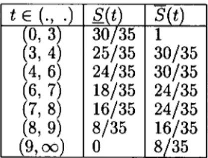
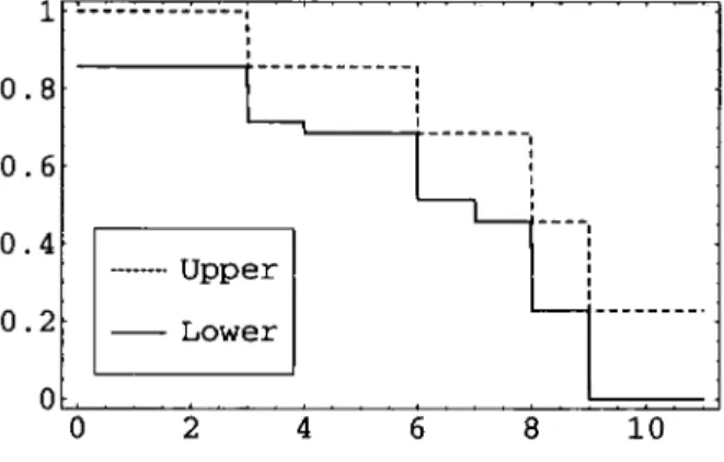
3.3 The lower and upper survival functions (Example 7) 59

3.4 Cervical cancer survival data (> t indicates right-censoring at t). . . . 61

3.5 M-function values for TA,I7 and P ( T ^ , i 7 G lA,i) (Example 8). . . . 62

3.6 M-function values for TB,I5 and P ( T B , I 5 e IBJ) (Example 8) 62

3.7 Lower and upper survival functions for cervical cancer example. . . . 63

3.8 Lower and upper survival functions for Example 3 67

3.9 Acute leukemia survival data (> t indicates right-censoring at t). . . . 71

3.10 Predictive probabilities for TB,22 (Example 9) 72

3.11 Predictive probabilities for T4,22 (Example 9) 73

3.12 Predictive probabilities for Tg (Example 10) 74

3.13 Predictive probabilities for Tg (Example 10) 75

4.1 The lower and upper probabilities for T59 € (Example 11) 89

4.2 Lower and upper survival function for grouped data (Example 11). . . 94

4.3 Event and censoring times per interval 96

4.4 Lower and upper predictive survival functions, and standard life table

estimator 96

4.5 Lower and upper predictive survival function for (oz, Oz+i) 96

4.6 Lower and upper predictive probabilities for T n+ i G I^, and lower and

upper expected values for 6^ in imprecise Dirichlet model 97

5.1 Relapse-free Survival Times for Hodgkin's disease patients ( > t

1.1 (a) Real time; (b) time T from entry ( X , death; Q, censoring). . . . 13

2.1 PL estimator of survival function (Example 1) 19

2.2 Ball bearings example: survival functions for T24 23

3.1 Upper and lower survival functions (Example 7) 60

3.2 Upper and lower survival functions (Example 8) 64

3.3 Lower and upper survival function, and the uniform BH survival

func-tion (Example 3) 68

3.4 Survival functions for ^4,17 (Example 8) 69

3.5 Survival functions for TB,ib (Example 8) 70

3.6 The upper and lower survival functions with ties (Example 9) 72

3.7 The upper and lower survival functions for (Example 10) 75

Introduction

1.1 Overview

Statistical analysis of lifetime data is a topic of considerable interest in areas such as medicine and engineering. The field has developed rapidly in the past half century, and many statistical methods for lifetime data have been presented. By studying these methods, we can find that most earlier methods mainly involved parametric models. An advantage of parametric models is that they are often specified by only a few parameters. However, it is often difficult to derive such parametric models, which considerably affects the use of parametric models. A classical method presented by Kaplan and Meier [46] proposed a nonparametric method for lifetime data. After that, nonparametric methods have been widely applied in statistical analysis for lifetime data.

We know that, in the study of lifetime data, incomplete observations due to censoring often occur. As the most common form of incomplete observation, right-censored data are considered in most nonparametric methods, such as the Kaplan-Meier estimator of the survival function. Other nonparametric methods introduced in Chapter 2, such as the 'standard life table estimator' [48] for grouped data, and Mantel's test [50] for comparison of two groups of lifetime data, present how to deal with right-censored observations in different problem situations. These nonparamet-ric methods have a common character on dealing with right-censored observations, that is they do not take all censoring times precisely into account.

All methods mentioned above are based on estimation of the survival functions, and they are not intended for prediction of a future observation, or other predictive inferences. Estimation is often important, but prediction also plays a key role in

real decision-making processes [1, 10, 37]. Talking of prediction, we may consider Bayesian prediction. Conventional Bayesian methods yield a predictive posterior distribution, using a prior distribution for a parameter. But in this procedure, the selection of a statistical model and a prior distribution may be difficult. Particu-larly, i f there is no appropriate model, Bayesian prediction becomes difficult. Hill

39] proposed the assumption ^(„) for prediction in the case of extremely vague a prior knowledge about characteristics of the underlying source of observations, sometimes it is also called low structure Bayesian prediction [38]. Based on the assumption i4(„), Berliner and Hill [6] presented a nonparametric predictive method based on lifetime data including right-censored observations. A disadvantage of their method is that they use so-called 'partial censoring information' instead of the exact censoring information, which makes a slight change to the censored data.

This thesis presents a new way to deal with censoring information in our non-parametric predictive methods. By generalizing Hill's a new assumption is presented, called 'right-censoring ^ ( n ) ' - Based on this new assumption, we obtain

predictive inferences which take all censoring times precisely into account. A t the same time, we can also extend these inferences to other predictive problems, such as grouped data and comparison of two groups of lifetime data.

1.2 Lifetime data

In statistical analysis, data may, for example, arise from the following situations: (1) The survival times of patients in a clinical trial; (2) The lifetimes of machine components in industrial reliability; (3) The duration of periods of unemployment in economics; (4) The lengths of tracks on a photographic plate in particle physics; (5) The number of years until death of people who have bought life assurance policies. The data in such situations are often referred to as 'lifetime data' even though the observations may not refer to lifetimes in the strictest sense. Mathematically we can think of a 'lifetime' as a one-dimensional non-negative random variable. Let

T denote the lifetime random variable, then T G [0,oo). Lifetime data are often encountered in both medicine and engineering applications such as those in cases (1) and (2) respectively. The study of lifetime data in engineering applications is normally referred to as reliability analysis, whilst in medicine we often talk about survival analysis. Cases (3) and (4) illustrate that lifetime data are encountered in a wide range of disciplines such as economics and science. Case (5) is an important

consideration when setting premiums for life assurance policies.

In order to determine lifetime data precisely, three basic elements are needed:

(i) A starting point for measuring time (the time origin); (ii) A finishing point for measuring time (ending event of interest); (Hi) A scale for measuring time. The time origin can be viewed as the starting point of the measuring process. The in-dividuals in the study may have diflferent time origins. For example, most clinical trials have staggered entry, and each patient's lifetime is measured from their date of entry into the trial (first time), rather than from the date of the first entry into the trial. For the end point, first there must be a defined event related to particular time points. For example, in medical work, this event could be death from a specific cause (e.g. lung cancer) or the recurrence of a disease after treatment. The scale for measuring time is often real (clock) time, but could also be the operating time of a system, the mileage of a car, or some measure of cumulative load encountered.

-X - X 1980 1985 1987 1990 ( a ) -X - X - X - O t=o t=10 ( b )

Figure 1.1 (a) gives the real times for ten individuals with staggered entry and follow-up until 1990, and using death as point event. Figure 1.1 (b) illustrates the lifetimes for these ten individuals respectively. I t should be noticed that seven of them are dead before 1990, and three of them are still alive at 1990. So we can ob-tain the exact lifetimes for those who are dead before 1990. For those who are still alive at 1990, we only know that their lifetimes exceed certain times. Such obser-vations refer to a special feature of lifetime data, these are known as right-censored observations and will be discussed in the next section.

1.3 Censoring

We review censoring, closely following Lawless [48]. Censoring arises in various ways. Formally, an observation is said to be right-censored at c i f i t is only known that the lifetime is greater than c. For example, when a patient has been given a certain treatment, a right-censoring time might arise i f the patient is still alive at the end of the time period set aside for observation. Similarly, an observation is said to be left-censored at c if it is known only that the observation is less than c; this situation might arise if a patient were put on test, but only checked for reaction every month. I f at the first check after one month, the patient is found to have died, then we only know that his lifetime was less than one month. In this example, i f the patient was found to have died between the second and third checks (that is, the patient was alive at the second check, but had died by the third check) then we would know that the patient had a lifetime between two and three months. This is an example of interval censoring. Obviously, right-censoring and left-censoring are two special types of interval censoring. As an incomplete observation in the study of lifetime data, right-censoring is the most common form. In this thesis, we present a nonparametric predictive method based on lifetime data, including right-censored observations. Throughout the thesis, except Section 3.7 (where left-censored observations are considered), we will refer to all lifetime data as 'event time', i f i t is a time at which the event of interest actually occurred, or 'right-censoring time'.

On analysing censored data, there are some important assumptions about the nature of the censoring and its relationship to the event process. Following Meeker and Escobar [52], we describe these assumptions. First, a censoring time can be random, but it is often a predetermined value due to practical reasons. For example.

in a life test experiment of n patients, a decision is made to terminate a study at a date on which not all patients' lifetimes will be known, then right-censored observations for such an experiment will occur. In order for standard censored data analysis methods to be valid, i t is necessary that the censoring time of an observation depends only on the history of the observed event process. Using future events to stop observation could cause bias. The second assumption is that censoring is non-informative. For right-censoring, this means that such an event is only known not yet to have taken place at the corresponding right-censoring time, and no further information with regard to the corresponding event time is available.

As censored data are often encountered in collection of lifetime data, undoubt-edly, we must be able to deal with it in statistical analysis. In Chapter 2, we will review some nonparametric methods, and discuss how they deal with right-censored data.

1.4 Outline of the thesis

This thesis considers nonparametric predictive inference for lifetime data including right-censored observations, based on the new assumption 'right-censoring /!(„)'. In Chapter 2 we briefly review some nonparametric methods presented for lifetime data and discuss how the right-censored data are dealt with in these methods. Hill's assumption A^n) is also reviewed in this chapter. In Chapter 3, we generalize Hill's and present the assumption right-censoring A(^n) (rc-^(n))- The assumption

rc-A(n) and corresponding nonparametric predictive inference (NPI) are the main topic of this chapter, and indeed of this thesis. They present a new way for dealing with right-censored data in the nonparametric situation. In Chapter 4, we apply rc-A(^n)

and N P I to grouped data with right-censored observations. We also compare our method with alternative nonparametric methods. In Chapter 5, we apply rc-A(„) and NPI to predictive comparison of two groups of lifetime data including right-censored observations, and compare our approach with an alternative nonparametric method. Finally, we summarize our main results, along with some concluding remarks, in Chapter 6.

Nonparametric inference and

right-censored data

2.1 Introduction

Nonparametric methods are widely used in statistics. In practice, they are often attractive as they allow more flexibility than the use of parametric models. As Hill [40] remarked: ' I n fact, nonparametric analyses represent the great majority of statistical situations, whilst parametric models are appropriate only in quite limited cases'.

In this chapter, we briefly review some nonparametric methods for lifetime data, and discuss how these methods deal with right-censored data. In Section 2.2, we introduce the classical nonparametric method by Kaplan and Meier [46]. As a non-parametric estimator of a population survival function, the Kaplan-Meier method [46] presents a tool for analyzing censored data. For nonparametric predictive anal-ysis, the assumption A^n) has been proposed by Hill [39]. In Section 2.3 we present Hill's A^n) and briefly discuss possible inferences based on this assumption. Although

A(n) does not apply to censored data, it provides an important tool for nonpara-metric predictive analysis. Later we will use this assumption to present our non-parametric predictive inference with right-censored data. Based on the assumption

A^n), Berliner and Hill [6] present a nonparametric method for predictive analysis in case of right-censored data, which is described in Section 2.4. Section 2.5 discusses 'grouped data', focusing on two methods, the standard life table estimator [48] and the method by Coolen [13], based on Walley's [58] imprecise Dirichlet model. These two methods are also used to compare with our nonparametric method presented in

Chapter 4. Section 2.6 reviews comparison of two groups of lifetime data with right-censored observations, and Mantel's test [50] is considered in this section. Later in Chapter 5, Mantel's test is used to compare with our nonparametric method. Finally, in Section 2.7 we briefly add a few concluding remarks.

2.2 Kaplan-Meier estimator

In this section, we discuss the nonparametric estimator of the survival function for data including right-censored observations, presented by Kaplan and Meier [46], which is also known as the 'Product-Limit' (PL) estimator. This method is widely used, and presented in about all textbooks on survival analysis, e.g. [23, 45, 48, 53, 55 .

Before we introduce the Kaplan-Meier method, we first give an important concept used in the method. I f the events of interest are the deaths of individuals, the risk set at time t is the set of individuals known to be alive (i.e. alive and uncensored) at time t, and denoted as n j . In this thesis, at an event or censoring time t, rit does not include the individual corresponding to the observation, so rij is always equal to the number of event and censoring times greater than t. In addition, we use Uf to denote the number of individuals known to be alive just prior to t.

Suppose that there are observations on n individuals, and there are k {k < n)

distinct observed event times ti < t2 < • • • < tk, where i t is possible to have multiple events at tj, let dj be the number of events at tj. In addition to the lifetimes ti,...,tk, assume that there are n - X l j = i r i g h t - c e n s o r e d observations for individuals whose event times are not observed. Let there be / different right-censoring times, ci < . . . < Q. The PL estimator of the survival function, on the basis of these observed data, is

s(t) =

n

where fitj is the number of individuals at risk just prior to tj.

The PL estimator is a step function, which is constant on [tj,tj^i), for j =

0 , 1 , . . . , A; — 1 with = 0, and decreases at event time tj by a factor (nt^. — dj)/hty

If the largest observation is at event time tk, then the PL estimator is zero on

[tk,oQ). I f the largest observation is a right-censoring at Q, then the PL estimator is a positive constant on [tk,ci), but for interval [cj,oo) i t is often left undefined.

On the interval [ 0 , t i ) , the PL estimator is equal to one. In the PL estimator, every drop of value happens at an event time, there is no change at censoring times. So we can say that censoring times do not have any direct effects on the PL estimate, their only effect is on the size of the later steps.

The PL estimator provides a nonparametric estimate of the survival function corresponding to the lifetime distribution for a population, and it is the Maximum Likelihood Estimator (MLE) [46], as such generalizing the empirical survival func-tion in case of no censorings. I t should be noted that, for the PL estimator to be the nonparametric M L E , the implicit assumption is made that attention is restricted to the class of all probability distribution functions [46]. The discrete model that underlines this estimator is described in detail by Lawless [48, Section 2.3].

Now we illustrate the PL estimator via an example.

Example 1

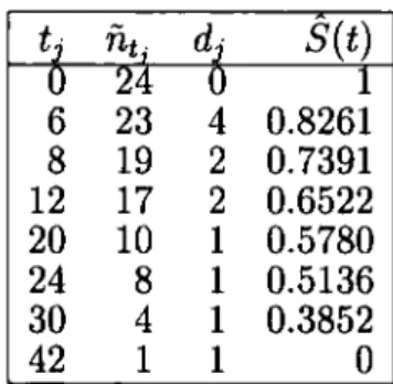
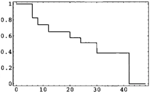
The data for this example are from the Dukes' C colorectal cancer patients of Mclll-murray and Turkic [51]. The data are on survival of 24 patients with Dukes' C colorectal cancer randomly assigned to receive control treatment. These survival times are being measured in months, and given in Table 2.1, together with the PL estimator S{t). Figure 2.1 is a plot of the PL estimator.

6 8 12 20 24 30 42 23 19 17 10 8 4 1 4 2 2 1 1 1 1 S{t) r 0.8261 0.7391 0.6522 0.5780 0.5136 0.3852 0

Table 2.1: Dukes' C colorectal cancer survival data.

The Kaplan-Meier method is regularly used to graphically present data including right-censored observations. Many nonparametric methods for inference based on lifetime data, for example, the standard life table estimator [48] for grouped data, are related to this method.

1 0.8 0.6 0.4 0.2 0 10 20 30 40

Figure 2.1: PL estimator of survival function (Example 1).

2.3 Assumption A^^) and imprecise probability

2.3.1 Overview of

The assumption was proposed by Hill [39, 40], for prediction in the case of extremely vague a prior knowledge about characteristics of the underlying source of the observation. Let f j , for i = 1 , . . . , n, be data values obtained by sampling from a population, and let t(i) be their ordered values (in increasing order of magnitude). Let Ti be the corresponding pre-data random quantities, so that the data consist of the observed values, Ti — ti, i — 1,... ,n. Following Hill [42], A^n) is defined as follows.

1. The observable random quantities T i , . . . , T „ are exchangeable. (In the original definition of A^n) [39], exchangeability was not included allowing more general situations.)

2. Ties have probability 0. (Generalization to include possible ties is straightforward, see Hill [40], but leads to more awkward notation.)

3. Given data ti, i = 1,... ,n, the probability that the next observation falls in the open interval = (i(_,),t(j+i)) is l / ( n + 1 ) , for all j =

0 ,. . . , n, where we define t^o) — —oo (or, for example, <(o) = 0 when dealing with non-negative random quantities) and t( n + i ) = oo.

It is clear that A^^) is a post-data assumption related to finite exchangeability

[30], see Hill [40] for a detailed presentation and discussion of and an overview

of related work, including important contributions by Dempster [31] and Lane and Sudderth [47]. Hill [42] presents a class of parametric models, called 'splitting pro-cesses', with a member which results exactly in v4(„) as posterior predictive assuming finite additivity, hence providing a nonparametric Bayesian justification for

A^n)-A natural interpretation of A^n) is in terms of ranks, namely the rank of the next observation amongst all observations will be equal to any possible value with probability l / ( n + 1 ) . Prior to the data {ti,..., f „ } , this is just an implication of exchangeability, so can be considered as a 'post-data version of exchangeability', the data carry information on location, but no information whatsoever on the rank of the future observation, which indeed corresponds to absence of prior knowledge.

De Finetti's representation theorem [30] uses a similar setting to justify a Bayesian framework for learning about an underlying parameter, and a probability distribu-tion for that parameter, but he relies on the assumpdistribu-tion that indeed there is an infinite sequence of random quantities involved, whereas our interest is mostly in inference on a single future observation. Even more, the Bayesian approach, as justified by De Finetti's [30] important results, explicitly needs a specified prior distribution, and together with the conditional independence of future observations (conditional on an unknown parameter) this adds quite a bit more structure to the data.

2.3.2 and imprecise probability

The assumption A(„) is not sufficient to derive precise probabilities for many pos-sible events of interest. However, i t does provide bounds for probabilities, by what is essentially an application of De Finetti's 'fundamental theorem of probability' 30] or Walley's 'natural extension' [57]. I n this situation, some related predictive inferences, based on the assumption A(n), can be expressed using imprecise proba-bility. In this subsection we review the related concepts and properties of imprecise probability, and describe -based imprecise probabilities which are bounds for

the predictive survival function in case of no censoring.

(I) Imprecise probability

The idea to use imprecise probabilities dates back at least to the middle of the nine-teenth century [8]. Since then, the use of imprecise probabilities has been suggested in many areas of statistics. Recently, there has been increasing activity in this area by researchers from widely varying backgrounds, resulting in a series of conferences

27, 28], special issues of journals [7, 24, 26] and a webpage [29 .

Extending De Finetti's theory [30] to imprecise probability, or more generally imprecise previsions, Walley [57] provides a rigorous generalization of the concept of probability, based on a behavioural interpretation of subjective imprecise proba-bility as bets with possibly differing maximum buying price P and minimum selling price P. Augustin and Coolen [4] propose an expression for imprecise probability. According to such an expression, the imprecise probability, for an event of interest

A, can be expressed by two optimal bounds,

P{A)=miP{A),

P{A) = snpP{A).

An important consequence for these two bounds is that P{A) and P{A) are conju-gate,

P{A)^1-P{A'), (2.2)

where A'^ is the complementary event to A. The conjugacy property can often be used to simplify the calculation of imprecise probabilities for events of interest and their complementary events (we will use this in Chapter 5).

Here we mainly introduced the related concepts and conjugacy property of im-precise probability. They will be referred to throughout this thesis. For a complete introduction and overview of imprecise probability, we refer to Walley [57].

( I I ) Imprecise survival functions

Now we illustrate how imprecise probabilities are derived for T„+i > t, giving im-precise survival functions based on the assumption ^(„) [17.

The survival function represents the probability for an individual of surviving past a certain moment of time. The survival function for an individual with random

positive lifetime T is defined as Srit) = P{T > t). Assuming observed event times for n individuals, ordered as t^i) < t^2) < • • • < ^(n), and denoting t(o) = 0 and ^(n+i) = OO) the assumption gives direct predictive probabilities for the lifetime

T„ + i of a further individual, at ty) this leads to predictive survival function for T^+i equal to

' 5 T „ + . {tu)) = for i = 0 ,. . . , n.

Without further assumptions it is not possible to give a precise value for this sur-vival function at times other than previously observed event times, as A^n) assigns probability mass l / ( n + 1) to the open intervals between observed event times, and to the intervals [ 0 , f ( i ) ) and (i(„),oo), but does not put any further restrictions on the distribution of the probability mass within each such interval. Therefore, the only inference we can derive at, without additional assumptions, consists of lower and upper bounds for the survival function, where we aim at deriving the maximum lower bound, denoted by 5, and the minimum upper bound, denoted by S, which are consistent with the probability assessment according to A(„). To derive S_{t),

one can shift the probability mass in the interval in which t lies to the left end-point of that interval (i.e. to the infimum value of the open interval), leading to

^ r „ + i W = ST^+AHJ+I)) = — - j - for i ^ {Hj),Hj+i)), with j = 0 ,. . . , n. This Srp^^^{t) is the optimal lower bound of ST^_^_^{t) based on v 4 ( „ ) , without

addi-tional assumptions. We call this S the lower survival function for T„+i. Similarly, one derives the optimal upper bound of Sr^+iit), called upper survival function S,

by shifting the probability mass per interval to the right end-point (the supremum of the open interval), leading to

Sn+At) = ST„+Akj)) = for i G (^o),^(J+l)), with j = 0, . . . , n . Notice that, for any t > i(„), we have Srj^^^^it) — 0 and Sr^+iit) = l / ( n + 1 ) , while for any value t in ( 0, t( i ) ) we have S_j'^^^{t) — n/{n + 1 ) and Sr^^^it) — 1.

Example 2 illustrates the lower and upper survival functions based on the as-sumption v4(„).

E x a m p l e 2

The following data are the ordered numbers of millions of revolutions to failure for each of 2 3 ball bearings [25, Section 2.9 .

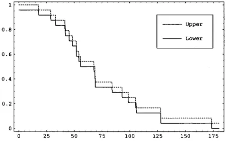
1 7 . 8 8 2 8 . 9 2 3 3 . 0 0 4 1 . 5 2 4 2 . 1 2 4 5 . 6 0 4 8 . 4 0 5 1 . 8 4 5 1 . 9 6 5 4 . 1 2 5 5 . 5 6 6 7 . 8 0 6 8 . 6 4 6 8 . 6 4 6 8 . 8 8 8 4 . 1 2 9 3 . 1 2 9 8 . 6 4 1 0 5 . 1 2 1 0 5 . 8 4 1 2 7 . 9 2 1 2 8 . 0 4 1 7 3 . 4 0

Based on these 23 observations, the assumption A(23) provides predictive prob-abilities for T24 as described above, leading to lower and upper survival functions for T24 as given in Figure 2.2. I t should be remarked that there are two tied obser-vations, at 68.64. Although A^n) is presented assuming no ties in the data, it can be seen that we now get a predictive point probability P(T24 = 68.64) — 1/24. We can think of these tied observations as being not really identical, with the tie being caused by rounding, with the probability for the very small interval between such two observations still equal to 1/24. One may, of course, doubt the correctness of such a predictive point probability for an apparently continuous random quantity. However, this point probability is actually caused by two identical values already observed, so it merely indicates that this value could well occur again.

0 . 8

0 . 6

0 . 4

0 . 2

25 50 75 100 125 150 175

Figure 2.2: Ball bearings example: survival functions for T24.

( I l l ) Inference based on A^n)

The position of -based inference in the theory of imprecise probability has been studied in detail by Augustin and Coolen [4]. These inferences have a predictive and nonparametric nature, which is referred to as nonparametric predictive inference

4]. Several examples of yl(„)-based nonparametric predictive inference have been presented, e.g. [3, 15, 16, 18 .

Inferences based on seem suitable if there is hardly any knowledge about the random quantities of interest, other than the first n observations, or, which may be more realistic, if one explicitly does not want to use such information. This may

occur, for example, i f one wants to study the (often hidden) effects of additional structural assumptions underlying statistical models or methods. Inferences based on such restricted knowledge have also been called 'low structure inferences' [38] and 'black-box inferences' [47]. In addition, A(„)-based inferences are entirely flexible, valid for few data, although high imprecision may be the fair price of only little information, and valid for many data as its asymptotics are closely related to those of the empirical distribution function.

2.4 Berliner-Hill method

By using the assumption v4(„), Berliner and Hill [6] presented a nonparametric pre-dictive method on the basis of data including right-censored observations.

Let T i , . . . , r „ be observable random quantities, assume that they are exchange-able, and that ties have probability 0. Suppose we have observations from these n

random quantities, consisting of u event times and v = n — u right-censored obser-vations. Let < t{2) < . . . < t(u) denote the order statistics for observed event times, and C(i) < C(2) < . . . < C(„) denote the order statistics for the right-censoring times. For convenience, let the random quantities T i ,. . . , r „ correspond to the event times t(i),..., and the random quantities Tu+j, for j = 1,..., D, correspond to the V censored observations C ( i ) , . . . , C ( „ ) . So the data consist of the survival times Ti = for z = 1,..., u , and censoring times Tu+j > C ( j ) , for j = 1,..., i?. Let T„ + i denote the next observation.

The censoring information provided by the right-censoring times, is called exact censoring information (ECI), and denoted as

ECl = {T,^j>c^jy.j = l,...,v}.

A further concept, called partial censoring information (PCI), is used in the Berliner-Hill method. For each censored observation C Q ) , j = 1,... ,v, let ij be the largest observed event time (or 0) smaller than C(j). Then PCI is defined as

PCl = {Tu^j>ij:j = l,...,v}.

Following the Berliner-Hill method [6], predictive probabilities for the next observa-tion can be derived as below.

Assuming A(n), let Zj denote the number of censored observations in interval (t(i),t(t+i)), and li = Ylk=o^i' f^'^ ^ ~ 0 , 1 , . . . , M , then the Berliner-Hill method specifies the following predictive probabilities

P ( T „ + i G ( 0 , i ( i ) ) I P C / ) = Ao,

P(r„+i G (%), t(i+i)) I PCI) - (1 - Ao) X . • • X (1 - Ai_i) X A„

for z = 1,..., w,

where

Aj = -, for i = 0,1,... ,u.

n- {i- 1) - li

Berliner and Hill [40] use PCI instead of ECI in their method, which allows them to deal with the censoring information by computation of the appropriate conditional probabilities for T„+i, conditioned on the observed event times and PCI for the ran-dom quantities corresponding to the censoring times, and using A(„) without further assumptions.

Berliner and Hill [40] also give upper and lower bounds of predictive probabil-ities for the next observation Tn+i- The upper bound is obtained by moving the censored observations in an interval (i(i), t(i+i)) just to the right of its left end-point, which is identical to replacing ECI by PCI. The lower bound is obtained by mov-ing the censored observations in (it(j), i(i_(_i)) just to the right of its right end-point. Although indeed this provides bounds for predictive probabilities for the next ob-servation T„_|_i, it adds some information to the data, which is not justified by these data.

Berliner and Hill [40] present a survival function based on PCI by assuming that the probability mass is uniform per interval, which leads to a continuous survival function. Let us denote this 'uniform Berliner-Hill survival function' by S^^^it),

then

sZ.(t) = ^lUki)) -

- ^ - ^ P ( r „ + i

(t(o,^(i+i))

for t e ( % , % + ! ) ) , where S^^Jt^i^) = 1 - E ; = I

^C^^+i

^T^Hiiho)) = 1, for i(o) = 0. Obviously, the uniform Berliner-Hill survival function beyond the largest event time is influenced by the choice of an upper bound for the random quantity T„+i. Without such an upper bound, a uniform Berliner-Hill survival function cannot be defined on this interval.

Example 3

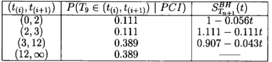
Suppose that we have three event times, 2, 3, 12, and five right-censoring times, 9, 10, 10.5, 11, 11.5. We assume A^s)- Table 2.2 gives the predictive probabilities for Tg according to the uniform Berliner-Hill method as outlined above.

(%,^(i+l)) P(T9e(%),t(,+i)) I P C / )

(0,2) 0.111 1 - 0.056t

(2,3) 0.111 1.111 - O . l l U

(3,12) 0.389 0.907 - 0M3t

(12, oo) 0.389

Table 2.2: The predictive probabilities and survival function, according to the uniform Berliner-Hill method.

Consider t = 8. There are two event times less than 8, and 5 censoring times and one event time greater than 8. This means that 6 out of 8 individuals will be at risk at the time 8. So, intuitively, the predictive survival function for Tg should be larger than the result derived in the example, STg{8) = 0.563. The uniform Berliner-Hill method uses PCI, that the random quantities, corresponding to censoring times, exceed t2 = 3, instead of exceeding ci = 9, C2 — 10, C3 = 10.5, C4 = 11, C5 = 11.5, respectively, and assumes that the probability mass in each open interval between event times is uniformly distributed. I t should be noticed that because there is not a finite upper bound for the observations, the uniform Berliner-Hill survival function is not defined on the interval ( 1 2 ,0 0 ) based on such a uniform assumption.

2.5 Nonparametric methods for grouped data

with right-censoring

2.5.1 Introduction

In reliability and survival analysis, data are frequently recorded in groups, with the time-axis partitioned into a finite number of intervals, and the data only consisting of numbers of event times and numbers of censoring times per interval. A well-known example of such data is the use of so-called 'life tables' [48]. In reliability contexts, such data may typically appear on lifetimes of non-critical components in systems, where e.g. once a month the components are inspected, showing i f they have failed

or not. In such situations, right-censoring could be due to component failures caused by competing risks, which are not the main failure modes under consideration, or by components being replaced due to a predetermined preventive replacement pol-icy. Grouping data is one of the most widely used methods of portraying lifetime data. Although grouped data have been used for a long time, the elaboration of their statistical properties has been a much more recent development because of the problems that censoring introduces [48 .

Suppose the time-axis is divided into A; + 1 intervals, — [az,az+i), z =

0,1,...,A;, with ao = 0, and a^+i = oo. For each member of a random sample of n individuals from the population, suppose that one observes either an event time or a right-censoring time. However, the data are grouped, so only the numbers of event times and censoring times in intervals are known, and not the exact event times and censoring times. Let be the number of event times in and

the number of right-censoring times in 7^. Let e — X]z=o ^ — 1^2=0*^2' ^o e -h c = n.

Based on grouped data, nonparametric methods are presented. Lawless [48] de-scribes the so-called standard life table estimator based on grouped data including right-censored observations, which is the nonparametric maximum likelihood esti-mator. However, in some sense, this method is arbitrary in adjustment of censoring mechanism, by effectively assuming that censorings took place at the middle of the interval. Other nonparametric methods, such as presented by Elveback [33] and Chi-ang [11], are derived on more formal grounds than the standard life table estimator, but there is still quite some arbitrariness in the adjustment to censoring. When there are relatively few censored data, or time intervals are not wide, there is not much difference between estimators such as Elveback's, Chiang's and the standard life table estimator. Coolen [14] adapted Walley's [58] imprecise Dirichlet model for grouped data including right-censored observations. In this method, censorings are assumed to take place at right-hand points of the time intervals. In this section, we mainly introduce two methods, the standard life table estimator [48], and the method by Coolen [13]. We will compare our new method for such data with these two methods in Chapter 4.

2.5.2 The standard life table estimator

We review the standard life table estimator, closely following Lawless [48]. Let the underlying survival function for grouped data be S{t). For = [a^, Cz+i), we define:

p, = P{T ^ h \ T > a,) and q, = P{T ^h\T>a,).

Obviously, = \ — p^, and = S{az+i)/S{az), so the survival function at a^+i is

S{a,+i) ^PoPi---p,, {or z = 0,l,...,k. (2.3)

Let Ua, be the number of individuals at risk at a^. The idea of the standard life table estimator is to employ (2.3) in obtaining an estimate of S{az+\), via the estimates of qz and p^. The usual procedure is as follows.

If there are no censored observations in I^, then an estimate of q^ is q^ = e^/ua^.

However, if there are censored observations in I^, e^/na^ might be expected to under-estimate qz. Therefore, an adjustment is required due to the censored observations. The standard life table estimator uses the following estimate of q^ in the situation that there are censored observations in 7^, that is

n„, - Czl2 n^^'

The denominator n^^ = — Cz/2 can be thought of as an effective number of individuals at risk over I^. Once estimates q^ and Pz = l — q^ have been calculated, we can estimate 5 ( 0 ^ + 1 ) by 5 ( 0 2 + 1 ) = poPi •• - Pz with ^ = 0 ,1 , . . . , A;.

It should be remarked that the adjustment for dealing with censored observa-tions is quite arbitrary in the standard life table estimator. In some situaobserva-tions other estimates of qz may be preferable. For example, i f all censored observations in Iz

are close to o^+i, the estimate qz = e^/na^ might be more appropriate, whereas if all censored observations in Iz are close to a^, qz — Cz/iua, - Cz) might be more

appro-priate. Clearly, any adjustments for dealing with censored observations effectively adds some additional information to grouped data, which is not justified by these data. Our method presented for grouped data in Chapter 4 does not need to add such eissumption for censored observations within 7^.

Example 4

Table 2.3 gives the standard life table estimator of the survival function for grouped lifetime data, given by Lawless [48 .

The example illustrates that standard life table estimator gives a survival func-tion estimate at points a^, for 2 = 0 ,1 , . . . , fc, with 5(0) = 1. The estimator of the

[az,ciz+i) ez Cz Qz Pz S{a,+i) 0,1) 356 60 0 356 0.1685 0.8315 0.8315 1,2) 296 48 0 296 0.1622 0.8378 0.6966 2,3) 248 30 0 248 0.1210 0.8790 0.6123 3,4) 218 28 35 200.5 0.1397 0.8603 0.5268 4,5) 155 19 49 130.5 0.1456 0.8544 0.4501 5,6) 87 12 41 66.5 0.1804 0.8196 0.3689 [ 3, oo) 34 34 0 34 1 0 0

Table 2.3: The standard life table estimate.

survival function at oo is assumed to be equal to 0.

2.5.3 The imprecise Dirichlet model for grouped data

We review the imprecise Dirichlet model for grouped data, closely following Coolen 13]. In this method, censorings are dealt with assuming that they are at times a^,

i.e. the censoring times within interval I^ are assumed to take place at the right-end point a^+i of this interval.

Walley [58] introduced an imprecise Dirichlet model related to multinomial data. Let the multinomial model have parameter vector 9 = {OQ, 9\, - - • , 6k), with Yl*i=Q — 1 and all 62 > 0, and

p{Tei,\d) = e„ fovz = o,i,...,k.

In a Bayesian framework, a Dirichlet distribution is a conjugate prior for this pa-rameter 6. A Dirichlet prior distribution is specified by the density function

7r{e \s,t)(xYle

z=0

with tz > 0 for 2; = 0 , 1 , . . . , and 1^2=0 = ^, and s is a parameter with s > 0. This prior distribution is uniquely determined by (s, t). Combining this prior distribution with the likelihood, based on e event times and c censoring times, leads to a posterior distribution as f{9\e,c,s,t). This posterior distribution is a generalised Dirichlet distribution, as introduced by Connor and Mosimann [12], and analyzed in detail by Lochner [49]. For statistical inference about 9^ in the Bayesian framework, the expected value E{9z\e, c, s, t) according to the posterior distribution can be obtained, see van Noortwijk et al. [56]. Clearly, E{9z\e,c,s,t) is a set of expected values for

6z, since i t is determined by {s,t). Based on such a set of expected values for 9^,

Coolen [14] derives the optimal lower and upper bounds for the expected value of

k

E{e,\e, c, s) = inf \^E{e,\e, c,s,t) \ ti > 0, ^ 1

i=0 k E{e^\e,c,s) = sup(E{e^\e,c,s,t) \ ti > 0, = l | , * i=0 E{eo\e,c,s)= J \ e -I- c-l- s E{9,\e,c,s) ^—J— ^ X I M ' ^ \, z = l , . . . , k - l as

\ efc + Ck-i J- Ej=i(ej+i + 9 ) + s ^

E{9k e, c, s) = X M r

and

eg + s ^(6*016,0,5)

e + c + s

The choice of s is discussed in detail by Walley [58], who shows that, when attempt-ing to model a lack of prior information, the choices s = 1 or s = 2 are reasonably cautious. The choice s = 0 would reduce the imprecise Dirichlet model to a precise Dirichlet model.

E x a m p l e 5

The example is from Coolen [14]. Suppose that the partition of the time-axis consists of A; = 5 intervals with Oi = 2, 0 2 = 4, 0 3 = 6 and 0 4 = 8. The number of event times in every interval are 1,0,0,2,0, and the number of censoring times 1,3,5,3,0. Table 2.4 gives the optimal lower and upper bounds of E{9z\e,c,s,t), for such grouped data.

The bounds for the expected value of 9^ in the imprecise Dirichlet model are Bayesian imprecise predictive probabilities for a future observation.

0,2) 2,4) 4,6) 6,8) 8,oo) e, c, s = 2) 0.1765 0.1255 0.1569 0.5378 0.6723 e, c, s = 1) 0.1250 0.0670 0.0852 0.4688 0.6250

E{6z e, c, s = 1) 0.0625 0 0 0.3125 0.4688 E{6, e, c, s = 2) 0.0588 0 0 0.2689 0.4034

Table 2.4: Bounds of E{9z\e,c,s^t) for Example 5.

2.6 Nonparametric methods for comparison of

two groups of lifetime data

2.6.1 Introduction

Comparison of two groups of lifetime data including right-censored observations is often required, for example in medical applications. For such comparison, an often used method is via parametric models for lifetime data, such as exponential dis-tributions, and then testing the equality of parameters. Alternative nonparametric method is also often used, such as Mantel's test [50], Gehan-Breslow's test [35, 36], and Breslow's test [9]. These nonparametric methods compare the unknown sur-vival functions from two groups of lifetime data, by testing a null hypothesis of equal survival functions.

Coolen [13] presented a nonparametric method for comparison of two different groups via predictive inferences for a future observation, based on A^n), but this did not allow censored data. In Chapter 5, we will generalize the method by Coolen [13], allowing right-censored data. In this section we briefly discuss Mantel's test [50], which we will compare with our method in Chapter 5.

2.6.2 Mantel's test

We review Mantel's test [50] for comparison of two groups of lifetime data, closely following Hollander and Wolfe [43 .

Suppose that there are Ua and Ub observations in groups A and B, respectively. Let Sa denote the underlying survival function of group A, and Si, the underlying

survival function of group B. Now combine the lifetime data from the two groups together and let i i < t2 < • • • < be the distinct event times of these two groups. Let ha,tk (^6,tfc) be the number of individuals from group A (B) who were at risk just before time tk, and let = ha^t^ + hb,t^, for 1 < fc < m. Let da,k {db,k) be the number of event times from group A {B) at tk, and let dk — da,k + db,ki for 1 < A; < m. Under null hypothesis HQ : Sa = Sb, the statistic

where

•C'a.fc — —:: and

T. dk{ht^ - 4 ) ^ a A " M *

ya,k — ZTT^ 7\

has approximately a A'^(0,1) distribution, if and are not too small and there are not too many censorings. The comparison of Sa and Sb is given by testing statistic, which is described as below,

1. One-side test of HQ against alternatives for which survival times for group B tend to be longer than those for group A. To test at the approximate a-level of significance, if Mc > Za (the critical value of a significance level), then reject Ho, otherwise do not reject;

2. One-side test of HQ against alternatives for which survival times for group A tend to be longer than those for group B. To test at the ap-proximate a-level of significance, if Mc < -Za then reject Ho, otherwise do not reject;

3. Two-side test of Ho against alternatives for which survival times for group B have a different distribution than that for group A. To test at the approximate a-level of significance, if \Mc\ > z&, then reject Ho, otherwise do not reject.

This is Mantel's [50] test. We illustrate this method via an example by Hollander and Wolfe [43, Section 11.7 .

E x a m p l e 6

The data in Table 2.5 are from a clinical trial on Hodgkin's disease, a cancer of the lymph system. We will also consider these data in Chapter 5. The following two

treatments were considered, (A) radiation treatment of the affected node and, (B) radiation treatment of the affected node plus all nodes in the trunk of the body. The data represent the relapse-free survival times in days. If a relapse had not occurred before the end of the data analysis, then the observation for that patient is right-censored. Treatment A Treatment B 86 822 173

>

>

>

>

>

>

>

>

>

>

>

>

>

>

>

>

>

>

>

>

>

>

>

>

>

>

>

>

Table 2.5: Relapse-free survival times for Hodgkin's disease patients (> t indicates right-censoring at t).

The test statistic in Mantel's test is Mc = 3.25, which gives an approximate one-sided P-value of 0.0006. Thus there is strong evidence that total nodal radia-tion is more effective than radiaradia-tion of affected nodes in preventing or delaying the recurrence of early stage Hodgkin's disease.

In Mantel's test, the censoring times within interval (ifc,<fc+i) do not have any direct effects on the calculation of Ea,k, their effects are on the calculation of Ea,k+i-We can say that Mantel's test is similar to Kaplan-Meier estimator in dealing with censored observations.

2.7 Remarks

Statistical inference related to informative censoring is an important topic, both theoretically and related to application. However, as remarked by Coolen [14], it seems that only quite complicated model assumptions or a direct subjective approach are suitable to deal with the kind of information on lifetimes that may arise.

based on theory of counting processes and martingales, an excellent overview is given by Andersen, et al [2]. The novel methods presented in this thesis are not directly related to counting processes and martingales, comparison with such methods is an interesting topic for future research.

From the above discussion, either common nonparametric methods or classical statistical methods, they are all not capable of taking censoring times precisely into account, when dealing with the censoring information resulting from such non-informative censoring mechanism. In the following chapters, we present a novel nonparametric predictive method for dealing with right-censored data, based on a non-informative censoring assumption.

Right-censoring A^^^ and

nonparametric predictive inference

3.1 Introduction

In this chapter a new nonparametric predictive method is presented based on data including right-censored observations. Basically, the method is an attempt to learn about a future observation from past observations, including right-censored data, while adding only few additional structural assumptions. The method is based on Hill's assumption A^n) [39, 40]. However, the presence of right-censored data re-quires further attention, which is the main topic of this chapter. In Section 3.2, some further assumptions related to A(„) are introduced and justified. Based on these assumptions, Section 3.3 presents a new assumption, which is called 'right-censoring (rc-74(„)). Section 3.4 presents 'nonparametric predictive inference'

(NPI) for a new observation, based on rc-A(„). In Section 3.5 this new inferential method is compared to the established methods by Berliner and Hill [6] and Kaplan and Meier [46]. Throughout the first five sections of this chapter we assume that there are no ties present in the data, to keep notation relatively straightforward. However, in Section 3.6 the possibilities for the treatment of ties are discussed. Section 3.7 considers an application of this new inferential method for data sets including left-censored observations, using our method for right-censored data and a monotone only decreasing transformation of the data.

3.2 Preparing for right-censoring A^^)

3.2.1 Introduction

In Section 2.3 the assumption v4(„) [39, 40, 42] was discussed, which provides a partially specified predictive distribution for a future observation given past obser-vations, consisting of exact event times. For lifetime data there are often right-censored data among the observations. Although Berliner and Hill [6] present a related nonparametric method for dealing with right-censored data based on v4(„), they replace 'exact censoring information' (ECI), i.e. the exact observed censoring times, by 'partial censoring information' (PCI), in effect shifting each exact censor-ing time back to the nearest smaller observed event time, enablcensor-ing inference on the basis of A(„) alone. The question addressed in this thesis is if E C I can be used, via a generalization of A(„).

In this chapter, the assumption A^n) is extended via a generalization called 'right-censoring A(„)' (rc-^(„)), which presents a partially specified predictive distribution for a future observation, given the past observations including right-censored data, and indeed allows the use of E C I . As the preparation for this generalization of ^(„), this section presents some assumptions related to A(n)- In Subsection 3.2.2 an assumption denoted by A^n) is presented, related to A(„), which assumes that the predictive distribution for a future observation consists of probability masses defined on two kinds of open interval, one is formed by consecutive event times and the other is formed by a censoring time and infinity. Dealing with the probability masses on intervals formed by censoring times and infinity requires further attention. Subsection 3.2.3 presents a further assumption called 'shifted-^(„)', which presents a partially specified predictive distribution for the random quantity related to a right-censored observation in case of a 'non-informative censoring' assumption, related to exchangeability of a right-censored observation with all other random quantities in the risk set at the censoring time. In Subsection 3.2.4 an assumption called 'right-censoring A(„)' (rc-A(„)) is presented, based on and s h i f t e d - f o r dealing with the probability mass on an interval formed by a censoring time and infinity.

Throughout this section (and indeed this entire chapter, except Section 3.6) we assume that there are no ties of any kind in the data set, so also no ties among censored observations, nor censoring times coinciding with observed event times. Suppose that the data available, and on which to base predictive probabilities for a future observation, are as follows.

D a t a notation:

Assume that information is available on n exchangeable nonnegative real-valued random quantities, Ti,T2, • • • ,T„. For n observations, consisting of u event times ^(1)) ^(2)i • • • J ^(u) and V right-censoring times C(i), C ( 2 ) , . . . , C(„), assume that 0 < t(i) <

t(2) < ... < t(u) and 0 < C(i) < C(2) < . . . < C(„) are the ordered data. In addition,

the notation t(o) = 0 and t(u+i) = oo is used, unless explicitly stated otherwise. Let = (^(t)) ^(i+1)), for i = 0 , 1 , . . . , M, and let c'j < 03 < . . . < c|. denote the ordered

censoring times within / j , where li is the number of censoring times in / j , of course these li are nonnegative and sum up to t;.

In Chapter 2 the assumption A(^n) [39, 40, 42] was discussed. A(n) provides a partially specified predictive distribution for a future observation given past obser-vations, and describes this predictive distribution via probability masses in open intervals between the observed event times. These probability masses are restricted to those intervals, but there are no further specifications or restrictions on the spread of the probability mass within such an interval. The generalization of yl(„), presented in the next section, will specify predictive probabilities in a similar way. Therefore, a notation for probability mass is introduced, which is called M-function.

Definition 1 (M-function)

A partial specification of a probability distribution for a real-valued random quantity

T can be provided via probability masses assigned to intervals, without any further

restriction on the spread of the probability mass within each interval. A probabil-ity mass assigned, in such a way, to an interval (a, 6) is denoted by MrCa, 6), and referred to as M-function value for T on (a, b).

The intervals in this definition can be of any nature, but in this thesis, when assuming no ties in the data, M-function values are only used on open intervals, which is the reason of presenting the definition with intervals denoted as {a,b). Clearly, all M-function values for T specified on all intervals should sum up to one, and each M-function value should be in [0,1]. This definition does not require all probability mass for T in (a, 6) to be specified in a single M-function value, but clearly one can find a minimal representation by using only a single M-function value for all probability mass specified in such a way to an interval. Predictive probabilities according to ^(„), for the next observation T^+i, can be specified by MT„+I (%), = l / ( n -I-1) for j = 0 , 1 , . . . , n.

Generally, once a partial specification of a probability distribution for a random quantity is available in terms of M-function values, optimal bounds (i.e. minimum upper and maximum lower bounds) for probabilities of events involving this ran-dom quantity can be derived, where the bounds often correspond logically to limits occurring when the probability masses within the intervals are moved towards the boundaries of the intervals.

3.2.2 Effect of right-censored data on

(I) T h e assumption A(n)

The assumption A^n) provides a partially specified probability distribution for a fu-ture observation T„+i, in terms of M-function values, based on n observed event times. But there might be right-censored observations among the data. In this situation, what is the effect of right-censored data on such a partially specified probability distribution for T„+i? This leads to the definition of a generalization of A(„), which is denoted by A(„).

Definition 2 ( i ( „ ) )

The assumption A(n) is that the probability distribution for a nonnegative random quantity T„+i, on the basis of data including u event times, f(i) < t(2) < . . . < f(„), and V — n — u right-censoring times, C(i) < C(2) < . . . < C(y), is partially specified by the following M-function values:

(i) ^T„+,(i(t),i(i+i)) = l / ( r i + 1 ) , for z = 0, l , . . . , u ; (ii) MT„+i(c(j),oo) = l/(n-|-1), for j^l,...,v.

We use the notation M to emphasize that these M-function values are based on the assumption A^n) to distinguish notation from M-function values based on

rc-A(n) later via this thesis.

The assumption A(„) partially specifies the predictive probabilities for a future observation via M-function values, in the case of right-censoring times among the observations, without any further assumptions. These probability masses are defined on two kinds of open intervals, one is formed by consecutive event times, and the other is formed by a censoring time and infinity. It is straightforward to see that, if

the data do not include any right-censored observations, so ?; = 0 and u = n, then

A(^n) is identical to A(n)- Let us consider an example to explain the assumption v4(„).

We use this as a didactic example throughout this chapter.

E x a m p l e 7

Suppose that we have data consisting of four event times, 3, 6, 8, 9, and two right-censoring times, 4 and 7. Let T7 denote a corresponding random quantity for a future observation.

According to A(6), the M-function values for are

MTr(0,3) = MTr(3,6) = Mr, (6,8) = Mrr(8,9) = MT.(9,OO) = 1/7 and

MT.(4,OO) = MT,(7,OO) = 1/7.

( I I ) Justification of A^n)

The justification of A^n), in relation to yl(„), is as follows. The intervals created by the observed events times, (^(i), i(i+i)), for i = 0 , 1 , . . . , m, are each assigned a probability mass of l/(n-|-1), by A^^)- Considering one such interval, the total mass in it could actually be more than l/{n + 1) due to the presence of one or more right-censoring times within this interval. However, any additional probability mass due to such right-censoring times would not necessarily be restricted to lie within this interval, without additional assumptions, indeed leading to M-function values on intervals from a right-censoring time to infinity. If there is a right-censoring time in interval (f(i), t(i+i)), then the unobserved event time corresponding to this right-censoring time perhaps could also have fallen in this same interval, in which case the M-function value l / ( n -H 1) assigned to (t(i),t(i+i)) would actually be assigned to a smaller interval, namely from to that unobserved event time. However, without any further assumptions on where such an observed event time would fall within the interval (t(j),<(i+i)), this probability mass l/{n+ 1) cannot justifiably be restricted <