Document downloaded from:
This paper must be cited as:
The final publication is available at
Copyright
http://link.springer.com/article/10.1007%2Fs10618-013-0308-z
http://hdl.handle.net/10251/49300
Springer Verlag (Germany)
Bella Sanjuán, A.; Ferri Ramírez, C.; Hernández Orallo, J.; Ramírez Quintana, MJ. (2014).
Aggregative quantification for regression. Data Mining and Knowledge Discovery.
(will be inserted by the editor)
Aggregative quantification for regression
Antonio Bella · C`esar Ferri ·
Jos´e Hern´andez-Orallo · Mar´ıa Jos´e
Ram´ırez-Quintana
Received: date / Accepted: date
Abstract The problem of estimating the class distribution (or prevalence) for a new unlabelled dataset (from a possibly different distribution) is a very common problem which has been addressed in one way or another in the past decades. This problem has been recently reconsidered as a new task in data mining, renamedquantification when the estimation is performed as an
aggregation (and possible adjustment) of a single-instance supervised model (e.g., a classifier). However, the study of quantification has been limited to classification, while it is clear that this problem also appears, perhaps even more frequently, with other predictive problems, such asregression. In this case, the goal is to determine a distribution or an aggregated indicator of the output variable for a new unlabelled dataset. In this paper, we introduce a comprehensive new taxonomy of quantification tasks, distinguishing between the estimation of the whole distribution and the estimation of some indicators (summary statistics), for both classification and regression. This distinction is especially useful for regression, since predictions are numerical values that can be aggregated in many different ways, as in multi-dimensional hierarchical data warehouses. We focus on aggregative quantification for regression and see that the approaches borrowed from classification do not work. We present several techniques based on segmentation which are able to produce accurate estimations of the expected value and the distribution of the output variable. We show experimentally that these methods especially excel for the relevant scenarios where training and test distributions dramatically differ.
Antonio Bella·C`esar Ferri·
Jos´e Hern´andez-Orallo·Mar´ıa Jos´e Ram´ırez-Quintana
DSIC-ELP, Universitat Polit`ecnica de Val`encia, Cam´ı de Vera s/n, 46022 Val`encia, Spain Tel.: (+34) 96 387 73 50
Fax. (+34) 96 387 73 59
Keywords Quantification ·Regression Quantification· Probability estima-tion·Segmentation·Distribution·Aggregation
1 Introduction
A common situation in data mining applications involves training a regression model predicting the expenditure, consumption, number of complaints, or any other numeric valuey. For instance, imagine that we have learnt a model for individual customer expenditure from a customer portfolioX1(i.e., a dataset) that corresponds to a specific region, business area and time period, as ex-tracted from a hierarchical multidimensional data warehouse. Eventually, we may want to apply the model to adifferentcustomer portfolioX2, e.g., a dif-ferent slice of the datamart for which we do not have the true value fory(i.e.,
X2 is an unlabelled dataset). In order to assess this second portfolio, some typical questions might be: (1) “what’s the expected average expenditure for the new portfolio?”, (2) “what’s the percentage of customers that will have an expenditure lower than 20 euros?”, (3) “what’s the typical expenditure for this portfolio?”
An answer to these questions can be given by just applying the regression model to each customer in the new portfolioX2, so leading to a set ˆY2, which makes up a continuous empirical distribution ˆp. With this distribution, the above questions are just expressed as (1) Eˆp[y] (i.e., the mean of ˆY2), (2) P r(y≤20|y ∈Yˆ2) (i.e., a tail of the distribution) and (3) the valuetfor which P r(y≤t|y∈Yˆ2) = 0.5 (i.e., the median).
The above example refers to the aggregation of a regression model, but the notion can also be applied to the aggregation of a classification model. In fact, the latter has received much more attention in the literature under different names, with the term class prevalence (or distribution) estimation being the most common (Neyman, 1938; Tenenbein, 1970; Alonzo et al, 2003). Many of these works focussed on how a small sample could be used to estimate the distribution of a bigger sample (‘double’ or ‘two-phase’ sampling) and not necessarily when the distributions change. Also, some of these works do not rely on a supervised model issuing an output value for every single instance in the dataset.
Forman (2005; 2006; 2008) presented the problem as a new supervised ma-chine learning task called ‘quantification’. Quantification (for classification) was defined as follows: “given a labeled training set, [. . .] induce a quantifier
that takes an unlabeled test set as input and returns its best estimate of the class distribution”(Forman, 2006). Quantification is characterised (and distin-guished from other distribution estimation problems) by how the problem is presented.
First, quantification focusses on cases where the training and test distribu-tions differ (a distribution shift), because otherwise the quantification problem would be pointless: if the training and test distributions are equal, the best estimation for the test set seems to be the observed empirical distribution on
0.0 0.2 0.4 0.6 0.8 1.0 0.0 0.2 0.4 0.6 0.8 1.0 train x y 0.0 0.2 0.4 0.6 0.8 1.0 0.0 0.2 0.4 0.6 0.8 1.0
test: no distribution shift, no concept drift
x y 0.0 0.2 0.4 0.6 0.8 1.0 0.0 0.2 0.4 0.6 0.8 1.0
test: distribution shift, no concept drift
x y 0.0 0.2 0.4 0.6 0.8 1.0 0.0 0.2 0.4 0.6 0.8 1.0
test: no distribution shift, concept drift
x
y
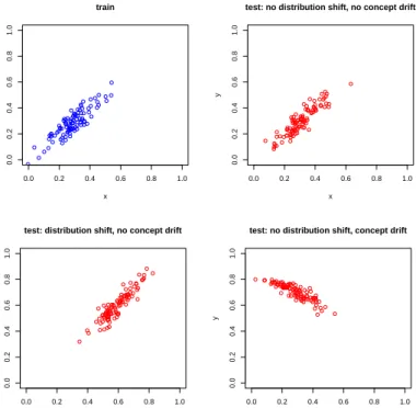
Fig. 1 An artificial example showing the applicability of quantification depending on the existence of (data) distribution shift and concept drift. Top left: actual distribution for the first batch (train). Top right: actual distribution for a second batch (test) where neither the concept nor the distribution have changed (p(y|x) andp(x) have not changed). While the estimation of the distribution may still be a problem when the number of training data is small, quantification is unnecessary here because other (and simpler) statistical approaches exist. Bottom left: actual distribution for a third batch (test) where the distribution (p(x)) has changed but the concept is the same (p(y|x) has not changed), so an estimatorˆp(y|x), trained on the first batch can still be useful. Quantification focusses on this problem. Bot-tom right: actual distribution for a fourth batch (test) where the distributionp(x) has not changed but the concept has drifted (p(y|x) has changed completely). Estimating the dis-tribution here is a much more difficult problem.
the training data, possibly using a smoothing approach or other statistical techniques. We then expect a change in the distribution. This may be a co-variate shift or a prior probability shift (Moreno-Torres et al, 2012), depending on whether the change originates on the covariates X or on the outputs Y. We will just use the term distribution shift for both cases. Importantly, a dis-tribution shift is different from a concept drift, where the very target function changes between training and test. Figure 1 shows this difference.
Second, the problem is presented with a labelled training dataset from which we can learn a supervised model or estimate other parameters, which are then used to estimate the distribution for the whole unlabelled dataset —available as abatchof examples.
A different question is how the problem is solved. A general and practical approach is performed by aggregating the predictions of an underlying
su-pervised model (a regression model, a classification model, or a conditional probability estimator ˆp(y|x)), which gives a prediction for each single instance
x. In other words, quantification is performed byaggregating the estimations for individual examples, with a possible adjustment of this aggregation, as we will see. This is especially appropriate in data mining applications where we already have (validated) predictive models, as well as applications with hierarchical data, where we train the model at the lower level and want to aggregate (roll-up) its predictions upwards, as usual in modern data ware-houses. This differs from cases where we may have a global estimator or other individual, but unsupervised, estimators, such as a likelihood estimatorˆp(x|y) or a joint distribution estimatorˆp(x, y). This choice of single-instance super-vised models is motivated by two observations: (1) predictive models are by far more common in data mining practice than likelihood or joint distribution estimators, and (2) the target function p(y|x) will be the same since we do not consider concept drift, while p(x|y) or p(x, y) are different whenever the distribution changes. This means that a supervised model estimating ˆp(y|x) can be preserved (differently fromˆp(x|y) or ˆp(x, y)).
Given this setting for quantification, the simplest approach is then to calcu-late the predictions for all the examples using the model and aggregate them. This is, in fact, an ideal solution when the supervised model is perfect. How-ever, many models are imperfect and biased (because of the difficulty of the problem: overfitting, underfitting, lack of data for some regions, and other fac-tors). In fact, Forman showed that, for classification quantification, the naive method “classify & count” does not generally produce a good approximation of the actual distribution for the dependent value y. In other words, a biased predictive model may lead to bad estimations of the overall distribution of the dependent value, especially when this distribution is significantly different from the distribution used for training.
Interestingly, however, some not-so-good models can be unbiased, and ag-gregating their predictions may lead to good quantification, or there might be some quantification techniques for biased models that could reduce or correct their bias and lead to good quantification. Forman summarises this (Forman, 2008): “it is sufficient but not necessary to have a perfect classifier in order to estimate the class distribution well”.
Since then, and given the large number of applications of quantification, new methods have been introduced that have improved the results for classifi-cation quantificlassifi-cation, such as an “adjusted classify & count” (Forman, 2008), “median sweep” (Forman, 2008), and many others (S´anchez et al, 2008; Xue and Weiss, 2009; Bella et al, 2010; Gonz´alez-Castro et al, 2012), either by using crisp classifiers, or soft classifiers (rankers or probability estimators).
The problem of quantification for regression may have the same large num-ber of applications as quantification for classification. Regression quantifica-tion addresses a very common situaquantifica-tion: the predicquantifica-tion of aggregated numeri-cal values such as sales, consumptions, duration, people, etc. However, to our knowledge, it has not been addressed in the context of distribution shift and using a base regression model.
While in classification this distribution is a discrete distribution (described as a set of probabilities for each class), in regression we can estimate a complete (empirical) continuous distribution and not only an expected mean. This also makes aggregative quantification for regression a more difficult task, as we will see, since the base regression models not only have bias on the location (the mean) but also have a tendency to compact the data and reduce the variability and dispersion of the output variable.
The goal of this paper is to develop new methods for regression quantifi-cation that can be applied over any predictive model built with off-the-shelf data mining software tools. As focussing on regression quantification, we will assume that the underlying predictive model is a regression model and we will concentrate most of our effort to thisdirectapproach. Also, and just for comparison, we will briefly explore the indirect approach of usingclassification
techniques applied to a discretised version of the problem.
We first explore the adaptation of several ideas from previous quantification methods, such as an “adjusted regress & sum”. However, as we will see, this adaptation produces poor results. A better analysis of the problem leads to a novel approach based on the idea of segmentation. Instead of estimating the whole distribution (which may have many different shapes depending on the application) and use this to correct the error of the regression model, we just use a more flexible approach. We segment the training distribution into bins and use the errors in each bin to adjust (scale) the regression model. Using these segmentation techniques and simple adjustments for location and spread we are able to get much better results than the “adjusted regress & sum” method.
Our contribution in this paper is then manifold. Firstly, we give a more solid and comprehensive view of the quantification problem for several tasks, leading to a taxonomy of quantification approaches with their corresponding evaluation metrics. This taxonomy also distinguishes the cases where we want to estimate an indicator (e.g., summarised statistic) of the distribution or the whole distribution. Secondly, we show that the problem of regression quantifi-cation is richer than the problem of classifiquantifi-cation quantifiquantifi-cation, because we move from a discrete output to a continuous output. The ideas which work for classification quantification do not work for regression quantification (such as global adjustment), using a direct approach, unless we convert the regression problem to a classification problem through discretisation as an indirect ap-proach. And thirdly, we propose new methods based on segmentation which are able to show good results even in the difficult distribution shift scenario we set in the experiments.
The paper is organised as follows. Section 2 introduces some notation, two examples and some previous work. From here we introduce a comprehensive taxonomy and a set of metrics for each quantification task in section 3. Then we focus on regression quantification in section 4, which analyses the problem more formally. We introduce several methods that are inspired by classifica-tion quantificaclassifica-tion and some new methods based on segmentaclassifica-tion, adjustment and spread, all assuming underlying regression techniques. In contrast, some
other indirect methods based on a discretisation of the problem and the use of classification quantification are also defined for reference. Section 5 performs a thorough experimental evaluation of these methods for the indicator esti-mation case and the distribution estiesti-mation case. Finally, section 6 closes the paper with a discussion of results and some future work.
2 Background
In this section, we will introduce some notation to express what quantification is precisely. The understanding of this problem will be helped by two exam-ples and a proper account of related work, including a short description of the methods which have been previously introduced for (classification) quantifica-tion.
2.1 Notation
We will deal with supervised (or predictive) problems, where the input and output domains are denoted byX andY respectively. An unlabelled dataset is any subset (actually a multiset) of X. A labelled dataset D is any subset of X×Y. We will use the terms DX and DY for the projections of D for
the input and output domains respectively. Occasionally, we will drop the subindex when clear from the context. Given an unlabelled or labelled dataset
Dof sizen=|D|, we will assume a (strict) order such that we can just refer to an example with its indexiin this order. Somewhat abusing notation we will expressi= 1. . . nori∈Dindistinctly. For theith example,yiwill denote the
true output value corresponding to the input valuexi. In this paper we refer
to both classification and regression problems. In classification, the output domain is a set of nominal values Y = {l1, l2, . . . , lc} usually referred to as class labels or simply classes; whereas in regression problems the output values are real numbers (Y ⊂R). A crisp model is any function m: X →Y. The estimation (or prediction) for inputxi is denoted by ˆyi. A soft or probabilistic
model is any function which returns a probability distribution for any given input valuex, i.e., a conditional probability estimatorˆp(y|x). For classification this is a categorical distribution and for regression this can be any continuous distribution. Typically,T rainwill denote the training dataset, whileT estwill denote the test dataset. In that follows, P r means probability, p denotes a probability density function o discrete probability distribution function andP
denotes a cumulative distribution function.
The (true) empirical (marginal) distributions for dataset D are given by the functionpDX(x) for the input values andpDY(y) for the output values.
In classification,
is a categorical probability distribution (which gives a probability or frequency for each class labell). In the binary case,⊕will denote the positive class and
⊖ the negative class. For instance, given a binary dataset D with a 80% of class⊕thenpDY(⊕) = 0.8.
In regression, pDY(r) is a probability density function for each real value r, with cumulative distribution function(PDY(r)):
PDY(r),P r(y≤r|y∈DY) =
Z r
−∞
pDY(y)dy (2) The expected value for this distribution is just the mean of DY, which is
denoted by: µDY ,E[DY] = Z ∞ −∞ y pDY(y)dy= Pn i=1yi |D| (3)
AndσDY denotes the standard deviation of the target values ofD, σDY ,
s Pn
i=1(yi−µDY)2
|D|2
Given an unlabelled dataset DX, we do not know pDY. Estimating this
probability distribution is precisely what this paper is about. Let us give a def-inition of quantification:
Definition 1 Quantification: Given a labelled training dataset T rain ⊂
X×Y for a supervised problemp(y|x), and given an unlabelled test dataset
T est, the quantification problem is the estimation ofpT estY fromT rain. IfY is a discrete set, then we have aclassification quantificationproblem, andpT estY is a discrete (categorical) distribution. IfY is a continuous set, then we have aregression quantification problem, andpT estY is a continuous distribution.
If this estimation is performed by aggregating the individual predictions ˆ
yi of a predictive model then we have an aggregative quantification approach.
The trivial solution for the aggregative quantification problem for classification is defined as: ˆ pT estY(l), Pn i=1I(ˆyi =l) |T est| (4)
whereIis the indicator function (I(true) = 1 andI(f alse) = 0). This solution is known as Classify & Count (CC). Similarly, the trivial solution for the quantification problem for regression is defined by the cumulative empirical distribution: ˆ PT estY(r), Pn i=1I(ˆyi≤r) |T est| (5)
which can be called Regress & Splice(RS). Note that this gives a value for each possibler, which determines an estimated distribution. In quantification,
(Perfect) individual predictions→(Perfect) distribution→(Perfect) indicators
Fig. 2 A schematic view of how much information (and effort) we require depending on the problem we want to solve. This gradation is illustrated by the arrows which become implications when we have perfect estimations.
we are interested in the whole distribution ofT estY or some of its indicators,
such as a mean or a median. Of course, this distribution or indicators can be well estimated by the use (e.g., aggregation) of very accurate individual predic-tions. However, it is important to realise again that we could also achieve good results from not-so-good individual predictions, provided they are not biased (locally and globally). As a thought experiment, consider that we scramble the predictions of a good regression model for an unlabelled dataset by just swapping an indefinite high number of predictions. After this, the distribu-tion is exactly the same, even though the regression model becomes awful for individual predictions.
This unidirectional relation is shown in Figure 2, where we illustrate that individual predictions are much more informative and require more effort than the estimation of the whole distribution. This is illustrated by the arrows, which show some kind of summarisation. Only when we have perfect estima-tions, these arrows become implications. Interestingly, as we go from left to right less information and effort is required. As a result, this schema also sug-gests that we do not always need to derive the indicators from the distribution, or the distribution from the individual predictions. In fact, on some occasions, it may be better to estimate the indicators directly.
One single and generally useful indicator that can be calculated from this estimated distribution (Eq. 5) is its expected value, which is an estimation for
µT estY above (Eq. 3),
ˆ
µT estY ,
Pn
i=1yˆi
|T est| (6)
which could be similarly called Regress & Sum (RS)1. In that follows, since
we will focus on the output domain and distribution, we will usually dropY
inT estY.
2.2 Examples: understanding quantification
Given the notation above we will see two specific examples that will help to better understand what quantification is, and how it works when aggregat-ing predictions from a base classification or regression model. We will also informally discuss some classical concepts that play an important role here, such as dataset imbalance or unevenness, overfitting, bias and variance, which will all be more formally addressed in section 4.1. Let us see an example for classification first:
1
We use the same acronym for Regress & Spliceand Regress & Sum, since both just aggregate the individual values with any further processing.
Example 1 A quantification problem in classification
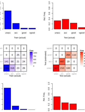
Consider a car renting company which assesses the suitability (acceptability) of a car (unacceptable, acceptable, good or very good) according to several characteristics.2 A classification model has been trained from data collected over a recent batch of cars which were supplied by the usual provider. Now, a deal is being negotiated with a new provider, which has given detailed informa-tion about the characteristics of all the cars in the new batch. The car renting company may be interested in calculating how many cars will be unacceptable. This is a quantification problem that can be solved by aggregating the pre-dictions of the classification model for this new batch of cars. Figure 3 (top) shows the class distribution for the first batch (T rain, left) and second batch (T est, right), which is not known by the car renting company and it is what we want to estimate. We see an important class distribution shift betweenT rain
and T est. In this case, we approximate the test distribution with a decision tree learnt from the training dataset. Its confusion matrix forT rainandT est
is shown in the middle row of Figure 3. If we apply the decision tree to all the examples in the test set and plot the predicted class frequencies, we get the histogram on Figure 3 (bottom, right). As we can see, this estimated distribu-tion significantly differs from the actual one. The estimadistribu-tion for class ‘good’ is almost perfect but a considerable error appears on ‘unacc’ and ‘vgood’. Notice-ably, we are not even able to guess which the majority class is for this dataset (it is ‘acc’ instead of ‘unacc’). In this case, quantification works well for some classes and poorly for others. Consequently, the goodness of quantification in classification can be interpreted in different ways, according to the goal of the quantification problem (estimating the frequency of one class, calculating the majority class, deriving the Pareto ordering of classes or deriving the whole distribution). Finally, it is interesting to take a look at Figure 3 (bottom, left). We see that the classification model applied to the training dataset (which was used for building the model) does not yield perfect quantification either. In fact, we can see that the model neglects class ‘vgood’ while overestimating ‘unacc’. This is due to the imbalance of the original dataset, where ‘unacc’ was highly prevalent. Typically, supervised models get biased in favour of cen-tral or majority values, because it is always preferrable in terms of expected error to bet for frequent values when there is some uncertainty. While this is good for classification metrics, we have that thisbiasis ultimately translated into the test set (or even magnified, since the model has more uncertainty on the test set). Taking this into account, we might think that getting a model which gives a perfect account of the distribution for the training set is the ideal solution, but this will generally make the model incur into overfitting, and the extrapolation to the test set will be poor —since we have a distribution shift. A possible idea to escape from this dilemma is to keep using supervised models which have been devised to have good generalisation performance as usual, and try to compensate the bias over the training set with some kind of
2
The example is elaborated, with some fictional elements, from the cars dataset in the UCI repository (Frank and Asuncion, 2010).
unacc acc good vgood Train (actual) Rel. Freq. 0.0 0.2 0.4 0.6 0.8 1.0
unacc acc good vgood Test (actual) Rel. Freq. 0.0 0.2 0.4 0.6 0.8 1.0 318 66 0 0 23 21 25 0 1068 141 0 0 26 24 15 0 unacc acc good vgood
unacc acc good vgood Train (actual) T rain (estimated) 0 250 500 750 1000 Freq 210 447 0 0 100 19 284 0 557 0 0 0 0 0 110 0 unacc acc good vgood
unacc acc good vgood Test (actual) T est (estimated) 0 100 200 300 400 500 Freq
unacc acc good vgood Train (estimated) Rel. Freq. 0.0 0.2 0.4 0.6 0.8 1.0
unacc acc good vgood Test (estimated) Rel. Freq. 0.0 0.2 0.4 0.6 0.8 1.0
Fig. 3 Top row: Actual class distribution for the first batch (training, left) and the second batch (test, right) of Example 1. Middle row: Confusion matrices for training and test. Bottom row: Estimated class distribution using the naive quantification methodClassify & Count.
post-hoc adjustment. This ‘adjustment’ is precisely what several classification quantification methods in the literature really do.
Let us now move to a regression problem.
Example 2 A quantification problem in regression
Consider a maternity ward that has collected data about baby weight at birth (dependent variable) for risk pregnancies, jointly with several features about the mother and her current and previous pregnancies (input variables). With these (training) data, a regression model has been trained in order to predict baby weight.3 In order to better plan the resources needed and the number
3
The example is elaborated, with some fictional elements, from the lowbwt dataset in the UCI repository (Frank and Asuncion, 2010), originally from (Hosmer and Lemeshow, 2000).
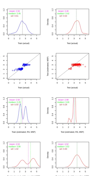
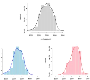
of expected complications, the hospital wants to estimate the distribution of weight births for the following month, according to a new group of pregnant women (test data) that the maternity ward is monitoring for future deliveries. This group has been reallocated from a different hospital (and borough), so we expect an important distribution shift but no important concept drift (see Figure 1), since the factors for delivery weights used in the model are assumed to have similar effects to any woman. So, the training and test distributions are different, mostly on their location, as seen in the first row of Figure 4. The second row of the figure shows how the model (a regression tree) behaves for the reference (train) and new (test) group of pregnant women. As we can see, this is not an excellent model; although there is some correlation between the actual valuesyand the estimated values ˆy, there seems to be some overfitting and underfitting, depending on the region (this is possible in regression trees). Note that the distribution of the estimated values differs from the distribution of the actual values for the training set (Figure 4, third row, left). The model compacts the predictions by paying less attention to those values which are at less dense regions or farther from the central part of the distribution. Also, the shape is now surprisingly bimodal, showing how distribution can be deeply modified just for the training set. In this case, because the original training distribution is relatively even (nearly symmetric), all this scarcely affects the location statistics for the estimated values, such as the mean or the median (2.50 and 2.25 versus 2.50 and 2.45 respectively).
When we compare the actual distribution for the test set (Figure 4, top right), with the naive approach byRegress & Splice(RS) (Figure 4, third row right), we see that the measures of location (mean and median) and spread (sd), as well as the distributions are different. Location is biased, variance is much lower and the shape is much more compact than the original. As we will see in section 4, we can improve the estimated location and spread by using several methods. Figure 4 (bottom left and right) shows better mean and standard deviation given by the methodakM (on the left using a smoothed distribution as in section 4.4, and on the right an ad-hoc smoothing over the mean assuming a normal distribution). In particular, the methodakM uses an
adjustment (correcting the bias), asegmentation(addressing the distribution estimation locally, by segments) and aspreadingmechanism.Adjustment(also mentioned in the classification quantification above) is justified because the bias is expected to be replicated (or magnified) in the test set (as happens for the RS method in this case, at least for the median, which is 0.20 kg lower for the training set but almost 0.40 kg lower for the test set). Segmentation
is justified to better account for all the regions for which we have data in the training set, more independently of their density.Spreading, as mentioned above, is justified because the distribution is too compact. The reason is easy to understand and is similar to the classification case. The use of the MSE
(mean squared error) as the metric for evaluating regression models makes that those predictions which highly deviate from the true value are strongly penalised. Consequently, for the most uncertain cases (which may come from the least populated regions) the model tends to output values closer to the
global mean. As a result, many (if not all) regression methods compact the predictions. We can see that, in this example, it is clearly the case (Figure 4, second and third rows). We will seeadjustment,segmentationandspreadingin subsequent sections. For the moment, we just want to highlight the importance of a good distribution estimation. For instance, the one on the right of the bottom row of Fig.4 is obviously more accurate for questions such as “how many births have a weight between 2,5 and 3,5 kg”, which can be answered with a value (45%), which is closer to the actual value (48%). Note that the other distribution estimation based on the methodakMgives a value of 21%, while the estimation given by the RS method is 93%.
The previous two examples show the nature of quantification when derived by aggregating a predictive model and brings out the similarities and differ-ences between quantification for classification and regression. These examples have also introduced some of the phenomena (bias and compactation) of the trivial aggregation methods RS. Both problems are shared by classification and regression, whenever the dataset is ‘uneven’ (in terms of class imbalance or in terms of irregular densities). Models tend to ignore peripheral (minority) cases, and this may lead to bias and compactation in the training data, which will also be present (and possibly worsened) on the test data. These previous insights are useful to better understand some previous techniques that have been developed for classification quantification, as we see below.
2.3 Previous methods for quantification
As mentioned in the introduction, the estimation of the class distribution for an unlabelled dataset has been addressed under different perspectives and applications. We mentioned some works on two-phase sampling, which referred to the problem as class prevalence estimation (Neyman, 1938; Tenenbein, 1970; Alonzo et al, 2003), where the goal and procedures were different from the setting we consider here. In some of these works, there was no distribution shift, but the need of estimating the class distribution of a population from a small sample (see Figure 1, top row). Also the estimation of the class distribution was not made by aggregating the predictions of a base classifier, but using a ‘measurement device’ (Neyman, 1938). In fact, this presentation of the problem is so frequent that it might have been solved in one way or another in the past, in different areas, especially from a Bayesian point of view (see, e.g., Chan and Ng 2006).
In the cases where we have a quantification problem as given by definition 1, with a distribution shift and an underlying supervised model constructed from the training set whose predictions can be aggregated for the test set, we have the setting first explored by (Forman, 2005, 2006, 2008). He developed different quantification methods (for classification) using the class predictions given by a crisp classifier or a ranker (a soft classifier outputting scores, probabilities or other estimations of the reliability of each class). The simplest one is the
0 1 2 3 4 5 0.0 0.4 0.8 1.2 Train (actual) Density mean= 2.50 median= 2.45 sd= 0.61 0 1 2 3 4 5 0.0 0.4 0.8 1.2 Test (actual) Density mean= 3.39 median= 3.42 sd= 0.54 0 1 2 3 4 5 0 1 2 3 4 5 Train (actual) T rain (estimated, M5P) 0 1 2 3 4 5 0 1 2 3 4 5 Test (actual) T est (estimated, M5P) 0 1 2 3 4 5 0.0 0.4 0.8 1.2 Train (estimated, RS, M5P) Density mean= 2.50 median= 2.25 sd= 0.50 0 1 2 3 4 5 0.0 0.4 0.8 1.2 Test (estimated, RS, M5P) Density mean= 2.98 median= 3.06 sd= 0.28 0 1 2 3 4 5 0.0 0.4 0.8 1.2
Test (estimated, akM−smoothd, M5P)
Density mean= 3.52 median= 3.90 sd= 1.02 0 1 2 3 4 5 0.0 0.4 0.8 1.2
Test (estimated, akM−smoothm, M5P)
Density
mean= 3.52 median= 3.52
sd= 0.60
Fig. 4 Estimations using a regression treefor Example 2. First row: actual distributions of the dependent value (y) for the training (left) and test (right) datasets. Second row: a plot of the regression model showing the correspondence between the actual values and the estimated values for the training and test datasets. Third row: estimated class distribu-tion using the naive quantificadistribu-tion methodRegress & Splice(RS) for the training and test datasets. Fourth row: estimated class distribution using a more sophisticated methodakM
for the test dataset: Left: using smoothing on the distribution. Right: using smoothing on the mean.
classify & count (CC) method (see Eq. 4). This method gives poor results since it underestimates the minority classes, as we have seen in Example 1. For this reason Forman introduced several other quantification methods by properly adjusting the threshold and, in some cases, also scaling the result. Theadjusted count (AC) method is an improvement of theCC method that estimates the true proportion of positivesdposby applying the equation
d pos=posd
′
−f pr tpr−f pr
where dpos′ is the proportion of predicted positives
P
i∈T estI(ˆyi=⊕)
|T est| . Forman
proposed estimating the true positive rate tprand false positive rate f pr by cross-validation on the training set. Since this scaling can give negative results or results above 1, the last step was to clipdposto the range [0..1].
Forman also defined a collection of methods based on selecting a classifier threshold over a soft classifier which, unlike theAC method, are determined from the relationship between tpr and f pr in order to provide better quan-tification estimates. For instance, the X method (which selects the threshold that satisfies f pr = 1−tpr), the Max method (which selects the threshold that maximises the difference tpr−f pr) or the T50 method (which selects the threshold wheretpr= 50%) are some of the methods in this group. The
Median Sweep(M S) method is a different approach that tests all the thresh-olds in the test set, estimates the number of positives in each one and returns a mean or median of these estimations. Finally, Forman proposed the Mix-ture Model (M M) (Forman, 2005) which calculated the distributions for the positive examples and negative examples separately and then joined them in a mixture. One of the conclusions of Forman’s works is that the best results were obtained withM S.
There have been a variety of methods using the probability estimations of a soft classifier (S´anchez et al, 2008; Bella et al, 2010; Gonz´alez-Castro et al, 2012). The first method in (Gonz´alez-Castro et al, 2012), HDx, is not an aggregative quantification method, because it does not use a base classifier, but just works on the distribution of the input variablesx. It compares likelihoods
p(x|y) (the authors use the term “class probability density functions”) for a validation and the test dataset with the Hellinger distance (using binning to approximate the integral in the definition of this distance). For a range of class proportions, it chooses the one which leads to the smallest distance. Since it discretises the input space, this method has limitations because of data sparsity and computational cost, when the number of features is high. An alternative aggregative quantification method,HDy, is also introduced (as an adaptation of HDx), which discretises the conditional probabilities for y
(instead of x). This makes it tractable when the number of features is high (and it also gives better results), because it constructs bins foryinstead ofx. Both methods rely on exploring a range of different values for the estimated class distribution, which works well for two classes.
Other methods use quantification to improve classification results or take advantage of a semi-supervised scenario (see, e.g, Xue and Weiss 2009). The
quantification methods in (Xue and Weiss, 2009) are mostly based on Forman’s original technique.
In (Bella et al, 2010) a collection of new quantification methods based on using the class membership probability (given by a probabilistic classifier) is introduced. The idea is based on the simpleProbability estimation & Average
(P A) method, where the class probability estimations are just averaged. This can be seen as just the probabilistic version of CC, since it considers the estimated class probability for each example instead of crisp decisions. Given a probabilistic classifierˆp(y|x), the average of the estimated probabilities for the positive class is calculated as:
ˆ pP A T est(⊕), P x∈T estˆp(⊕|x) |T est|
Logically, as in the CC method, if the proportion of positive examples in the training set is different from the proportion of positive examples in the test set, the result obtained by theP Amethod will not be satisfactory in general. So, as in the AC method, the idea is to use a proper scaling. The Scaled Probability Average (SP A) method (Bella et al, 2010) consists in applying the scaling over the test set that makes that the positive probability average for the positives in the training set, denoted by T rain⊕, is 1 and that the
positive probability average for the negatives in the training set, denoted by
T rain⊖, is 0. Therefore, this scaling transforms the estimation given by P A
so that thepositive probability average for the positives(ˆpT rain⊕(⊕)) is 1 and
thepositive probability average for the negatives (ˆpT rain⊖(⊕)) is 0. Formally,
SP Ais defined as: ˆ pSP AT est(⊕), ˆ pP A T est(⊕)−pˆT rain⊖(⊕) ˆ pT rain⊕(⊕)−pˆT rain⊖(⊕)
The results in (Bella et al, 2010) show a significant improvement over Forman’s methods.
3 Beyond classification: a comprehensive view of quantification and its evaluation metrics
The examples and the previous work seen in section 2 suggest that the quan-tification problem is multifaceted. Consequently, it can be studied according to several characteristics. This analysis leads to a comprehensive taxonomy and a set of evaluation metrics for each case, as we present in this section.
3.1 A taxonomy of quantification problems
We will consider two characteristics which critically determine the quantifica-tion problem. First, as already seen, quantificaquantifica-tion can be defined whenever we have a supervised dataset, be it a classification or regression dataset. In
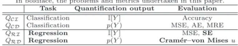
Table 1 Taxonomy of quantification tasks.
In boldface, the problems and metrics undertaken in this paper. Task Quantification output Evaluation
QCI Classification I[Y] Accuracy
QCD Classification p(Y) MSE, AE, MRE
QRI Regression I[Y] MSE,SE
QRD Regression p(Y) Cram´er–von Misesu
fact, other predictive tasks such as categorisation, hierarchical classification or ordinal regression can also lead to quantification problems.
A second characteristic is how much detail about the aggregated output we require. For instance, we may only be interested in the expected value of the output, or just a single indicatorI(any summary statistic, such as measure of location or spread, or some other function of the distribution). For instance, in classification, this could be the mode, or majority class. In regression, this could be the mean, as in Eq. 3 or 6, or the median. In other cases, however, we may require a full distribution of the output value, which is a categorical distribution in classification, as in Eq. 1 or 4 and a continuous distribution in regression, as in Eq. 2 or 5.This dimension allows us to apply a variety of different methods to solve the quantification problem. The distinction between indicators and distribution is motivated by the fact that it is usually easier to estimate a good indicator than to estimate the whole distribution well, because the latter requires more information, as seen in Fig. 2, and the techniques may take this into account4.
We will consider two options for the two characteristics above (classifica-tion and regression problems, and the quantifica(classifica-tion goal as a single indicator or a whole distribution), which will be represented by the lettersC|Rfor clas-sification or regression, andI|D for indicator or distribution. This gives four possible combinations and leads to a taxonomy of quantification tasks as shown in Table 1. This taxonomy broadens the scope of quantification, and can be useful for distinguishing research context for future reference.
For each problem in the taxonomy, different quantification methods can be defined depending on the underlying predictive model used to estimate the quantification output. It is not the same to solve quantification problems when we only have the estimation of the output value (ˆy) for each example as when we have posterior probability estimates provided by the model (ˆp(y|x)). Many classification techniques today are able to generate (soft) probabilistic models, and there are techniques for calibrating (Platt, 1999; Zadrozny and Elkan, 2001; Bella et al, 2009a,b, 2012) these probabilities which may have a positive effect on the quantification task. However, most regression techniques are still usually crisp and only output the estimation ˆy. It is true that some techniques can accompany each single prediction with the standard error, a reliability measure or a confidence band, but it is not clear how to incorporate
4
In this paper the methodology for indicators and distribution is the same (except for some minor specific techniques, mostly at the end of the process), but this could be dif-ferent in the view that some indicators require less information and effort than the whole distribution.
this information in the quantification problem. For instance, a conditional density estimatorˆp(y|x) would lead to the understanding of quantification for regression as a distribution mixture.
In this paper we focus on methods for solving cases QRI andQRD using
crisp models. We exclude from this paper those methods based on probabil-ity estimations because they require a soft regression model or a conditional density estimatorfˆ(y|x) (Hwang et al, 1994; Hyndman et al, 1996).These esti-matorsare usually non-parametric(as the shape of the true distribution is not known). As a result, many are proneto overfitting for small or medium-sized datasets(Hwang et al, 1994), and suffering from a number of limitations (for instance, some approaches are restricted to only one or two input variables, such as R’s hdrcde package, Hyndman et al 1996, and they do not handle
nominal variables appropriately). This goes beyondthe usual situation a data mining practitioner may face with a data mining tool, where she usually works with predictive models when training data is presented in a supervised fashion
with attributes of many different types and possibly missing values. Typically, supervised (crisp) regression models are more robust (and faster) in these sce-narios.
Finally, the taxonomy is also useful to clarify which evaluation metric is used for each case, as we see below.
3.2 Quantification evaluation metrics
We will start by reviewing the evaluation metrics for classification quantifica-tion. This set of metrics is shown in the last column of Table 1. Many previous works (Forman, 2005, 2006, 2008) on quantification for classification have used the absolute error (AE) for problemQCD, sometimes referred to as mean
abso-lute error (MAE), when aggregated over several repetitions or datasets. More precisely, the global AE for each class is the absolute difference of the propor-tion of elements for each classj in a test set T est (ˆpT est(j)) and the actual value:
AET est(j),|pT est(j)−pˆT est(j)|
and for all the classes we have themacro-averagevalue (equal to the micro-averagevalue for two classes):
AET est , 1 c X j=1..c AET est(j)
Any metric will provide a particular different view of the deviation from the actual value, and variants exists especially for normalising results when sev-eral repetitions and datasets are used in an experimental setting. Other met-rics used for classification quantification are the (mean) relative error (MRE) (Gonz´alez-Castro et al, 2012), which is equal to AE divided by the true positive proportion, or the squared error (SE), known as MSE in (Bella et al, 2010). Finally, since in classification we really estimate probabilities, a natural choice
might seem to use measures to compare probabilities, such as cross entropy. Clearly, the choice of a particular metric has its pros and cons, and may differ in being symmetric or not about the errors and paying more or less attention to the minority classes.
In case we are interested in determining which the majority class is (a single indicator, QCI), we suggest the use of a true/false metric indicating
whether the majority class has been identified (similarly for other indicators such as the minority case). Note that a quantifier with a good AE (or SE) does not necessary imply that the majority class is correctly identified, especially in multi-class problems.
This overview of metrics for classification quantification suggests that we may also have many different options for regression quantification. We will first consider the problems which output the mean (or other indicator) for the output value (QRI in Table 1). Since this is a numerical value which needs
to be compared to the actual mean, we use a typical measure for assessing the deviation with respect to a magnitude, the squared error. If we denote by
I(YT est) the true value of the indicator (e.g., the mean, the median, etc.) for
the test or deployment dataset, andI( ˆYT est) the estimated value for the same indicator, we define the squared error as follows:
SET est,
I(YT est)−I( ˆYT est)
2
For practical reasons, especially when the measure is used for an experi-mental evaluation of many repetitions and datasets (as in this paper), we may prefer to normalise the above measure to make values being less dependent of the magnitude range of the data and more commensurable among different datasets. In this paper, we will use the Squared Error (SE) seen above but normalised by the variance of the training setT rain, denoted by V SE:
V SET est,
I(YT est)−I( ˆYT est)
2 V arT rain(Y)
This normalisation by the variance is useful when magnitudes are aggregated for several repetitions, datasets or techniques. In pairwise statistical compar-isons, however, this normalisation has no effect.
Finally, we need to determine an appropriate evaluation metric for case
QRD in Table 1. Since we need to compare the estimated distribution with
the true one, we need metrics for comparing distributions, usually called diver-gences. However, many of them cannot be applied to empirical distributions, because the density function in some places equals 0. Consequently, empirical distributions are compared by using their cumulative distribution functions. A very simple statistic for comparing two empirical cumulative distributions
FV and FW is the two-sample Kolmogorov-Smirnoff (KS) statistic, which is
defined as:
KS,max
However, since the two-sample KS statistic is only based on the point where both distributions differ most, it disregards the shapes of the distributions. A more refined alternative is to take an average (or an integral), instead of a maximum. This is just the Cram´er–von Mises statistic (two samples) (An-derson, 1962). In particular, from the L1–version (Xiao et al, 2006a,b) we just need theU value, which can be easily calculated from the empirical data
YV =v1, v2, . . . , vn andYW =w1, w2, . . . , wmas follows:
Let us consider thatYV andYW are sorted in increasing order. We define
byYV W ,YV ∪YW and we also consider it is sorted. Letr1, r2, . . . , rn be the
ranks of the elements ofYV in YV W and lets1, s2, . . . , smbe the ranks of the
elements ofYW in YV W. Then: U ,n n X i=1 (ri−i)2+m m X j=1 (sj−j)2 which is normalised as u = U
nm(n+m). This value u (the u-statistic) will be referred to as the cvmumetric, which ranges between 0 and 2 (4/3 when n
is large). It is lower the more similar the two distributions are. For instance, thecvmumetric of the distributions on the right plots of the third and fourth rows in Figure 4 with respect to the true distribution for the test set (top right plot) are 0.41 and 0.18, respectively.
4 Regression quantification methods
Now that the place of quantification for regression in the family of quantifi-cation tasks has been clarified, as well as its evaluation metrics, we are ready to focus on problems QRI andQRDin Table 1. As in the classification case,
quantification is meaningless for those applications where the training and test distributions always match. In fact, if this were the case, the perfect solution forQRIin Table 1 would be just to estimate the indicator on the training set.
For instance, if the indicator is the mean, theTest to Train(T T) method just assigns the “same mean”, simply defined as:
ˆ
µT T
T est ,µT rain
where µT rainis an instance of Eq. 3 for the training set. Clearly, this can be
adapted for any indicator, such as the median. In the experiments in section 5 we will use the same acronym T T, for the corresponding “same median” version of the method. This method is just included as a baseline or reference, since we will focus on methods which account for a distribution shift.
Similarly, we can define a method called Test to Train (also denoted by
T T), which just ‘copies’ the distribution from the train to the test set and will be used as baseline for theQRD problem. The method just uses they values
in the training as the empirical distribution for the test. Note that there is no mapping between examples (as in other methods where the predictions are modified). In fact, the sizes of the training and test are usually different (which is not a problem for thecvmumetric seen in the previous section).
4.1 Analysing overfitting, bias and variance
Before presenting some more elaborated techniques, we analyse the regression quantification problem better to see how to take advantage from an underlying supervised model. Typically, regression models are trained (and evaluated) to minimise their mean squared error (MSE). From here, we can analyse the performance of a model with the classical (see, e.g., Hastie et al 2009; Flach 2012) bias-variance decomposition ofoneexample forallpossible datasetsD:
E{D}[(y−yˆ)2] = (E{D}[ˆy]−y)2+E{D}[(ˆy−E{D}[ˆy])2]
= (E{D}[ˆy−y])2+E{D}[(ˆy−E{D}[ˆy])2]
= (Bias{D}(ˆy−y))2+V ar{D}(ˆy)
where E{D} denotes the expected value for all possible datasets. The above
decomposition is usually a way to understanding overfitting as high variance: thepredictionsvary very significantly when we change the dataset, i.e., when we move from training to test. Underfitting is usually understood as high bias. At first sight, it may seem that a good regression model for quantification needs to have low bias. However, we cannot ignore the variance, especially because we have a data distribution shift. So, also for quantification, a good compromise between overfitting and underfitting must be found, because both are harmful for the extrapolation for new unseen areas. One thing that can be observed from the previous decomposition is the effect of outermost predictions. One can think that outermost overestimations are not harmful provided they are usually accompanied by a balanced proportion and magnitude of outermost underestimations. While this might be true for non-quadratic errors because they cancel, it is not true forMSE, as shown by both components. This is the reason why most regression techniques output predictions whose variance (i.e.,
V ar(ˆy)) is lower than the actual variance (V ar(y)), whereV arhere refers to the variance of all the examples in one dataset. This phenomenon seriously affects the spread of the predictions, leading to more packed predictions. As a result, regression models trained to minimise theMSE will need to be spread out (the shape of the distribution should be widened) in order to resemble the actual distribution, as we saw in Figure 4. The method introduced in section 4.4 is precisely based on smoothing the distribution such thatV ar(ˆy) =
V ar(y).
While the previous decomposition gives us some understanding about spread, it gives us few clues about the location of the estimated distribu-tion. For this purpose, it is more insightful to make the same decomposition of
allexamples ononedataset, since it is the result for all examples what counts for quantification, as follows:
= (E[ǫ])2+E[(ǫ−E[ǫ])2] = (Bias(ǫ))2+V ar(ǫ)
whereEdenotes the expected value forallthe examples inonedataset, and the error is denoted byǫ=y−yˆ. Note that now the variance refers to theerrors, not the predictions. Just focussing on one dataset, we cannot get information about overfitting and underfitting, but we can see other phenomena. We see that if the model givesBias(ǫ) = 0 then the mean of the errors will be zero — even if the errors may still be non-zero individually. This zero bias means that the mean will be perfectly estimated for that dataset. If the indicator function we are interested in is the mean, then we would get perfect quantification. Consequently, we want regression models such thatBias(ǫ) = 0. We can see clearly that if we add a constant s to all the predictions, we get a different
Bias(ǫ) but equal V ar(ǫ). It is then natural to expect that many regression techniques try to setBias(ǫ) = 0 by calibrating the model in this way. In fact, some linear regression techniques ensure Bias(ǫ) = 0 on the training set by definition, because the MSE is minimised5. Other techniques, however, may give slightly uncalibrated models for the training set,because theasymmetry of the training set forces the technique to unbalance the estimations for risk minimisation. Independently of the regression technique being used, we can always find the optimal constantsfor a dataset, by just settingsequal to the bias:
s=Bias(ǫ) =E[ǫ] =E[y−yˆ] =E[y]−E[ˆy] (7)
which just subtracts the mean of the actual values with the mean of the esti-mated values. It is also expectable that since the errors are usually higher on a test set,this valuesmay be higher for the test set than for the training set. This will be the basis of the adjustment methods below.
Finally, while a global adjustment may solve some cases, the bias can vary significantly between the central areas of the distribution and the outermost values. Typically, outermost values, as mentioned above, are usually pushed to the centre. This means that lowy values will typically lead to negative bias, and high y values will typically lead to positive bias. This suggests the use of adjustment constants customised for different regions of the distribution, leading to the segmentation methods in section 4.3.
5
As a mean-unbiased estimator minimises squared loss, a median-unbiased estimator is a different choice which minimises the absolute error.
4.2 Methods based onRegress & Sum
The simplest method for estimating the mean using an underlying regression model is the Regress & Sum (RS) method we defined in Eq. 6 but applied to the test set, which we will denote by ˆµRS
T est. TheRS method can handle a
distribution shift, but it depends on the quality of the training data sample (it must be representative of the overall domain) as well as on the quality of the regression model. Otherwise, the estimation might even be worse than the
T T method. This is similar to the problems already observed for theClassify & Countmethod in classification quantification.
In a quite similar way as the AC method (Forman, 2008) is an adjusted improvement of theCC method, or asSP Ais a scaled adjustment of the naive
P Amethod (Bella et al, 2010), we can follow the same idea in regression. In order to do this, we need to calculate the average of the true values for the
T rain set, µT rain. We also need to calculate the average of the estimated
values, i.e., ˆµRS
T rain (an instance of Eq. 6 for the training set). Now, we can
derive the error bias (Bias above, in what follows denoted by B) for the training set as follows:
BRS
T rain,µT rain−µˆRST rain
With this valueBwe can adjust any method, following Eq. 7. For instance, theAdjusted Regress and Summethod (aRS) is just:
ˆ
µaRS
T est,µˆRST est+α·BT rainRS (8)
where αis a parameter that makes the adjustment more or less intense, mo-tivated by errors being expected to increase for the test set, as discussed in the previous section. This value can be estimated from the use of a regression technique on similar problems, or can be set to a fixed constant independently of technique and problem, as we do in this paper. Note that whenα= 0 this is equivalent to theRSmethod.
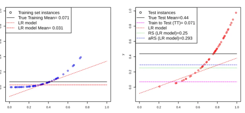
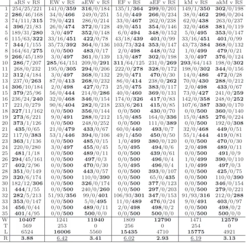
Figure 4.2 shows a simple example which illustrates how the methods de-scribed in this section work. We use a simple regression problem with only one attribute. We split the data into two sets of the same size,T rain and T est, but different distribution. On the left side of the figure we can see theT rain
dataset (points as blue circles). The dotted red line represents the model built from the training data using a linear regression method. The solid black hor-izontal line represents the average of the actual valuesy for the instances in the T rain set (0.071). The dashed red line shows the average of the linear regression model (0.031). The difference between these values indicates that the regression model is not calibrated with respect to the training instances. This slight difference will be used by the aRS technique. On the right side of Figure 4.2 we include the result of the application of theRS method over theT est set and the results of using theaRS (withα= 1) method with the same test dataset. We can see the different data distribution betweenT rain
0.0 0.2 0.4 0.6 0.8 1.0 0.0 0.2 0.4 0.6 0.8 1.0 x y
Training set instances True Training Mean= 0.071 LR model LR model Mean= 0.031 0.0 0.2 0.4 0.6 0.8 1.0 0.0 0.2 0.4 0.6 0.8 1.0 x y Test instances True Test Mean=0.44 Train to Test (TT)= 0.071 LR model
RS (LR model)=0.25 aRS (LR model)=0.293
Fig. 5 An artificial example y = x3
showing how several methods in section 4.2 work. Training and test are sampled from 100 examples with a triangular distributions overxin [0.1] with a 50/50 proportion. Left: Train data (mean = 0.07) and the regression model. Right: Test data (mean = 0.44). TheRS method and theaRS method (withα= 1) are shown.
shown. The solid line expresses the value of the mean of the test dataset, i.e., the actual average value. The RS method using the linear regression returns a value (0.25), shown as a green dotted horizontal line, which is slightly below the actual one (0.44). However, it is much better than theT T method (0.07). Finally, the blue dashed-and-dotted horizontal line shows the result of using the aRS (with α = 1) method with the same test dataset. Given that the linear regression is not calibrated with respect to the training data, there is a correction that modifies the estimated value for this technique to 0.293.
The previous methods RS and aRS have been presented to address the
QRI quantification task in Table 1 where the indicator is the mean. The idea
can be easily extended for the median and other indicators. Also, the RS
and the aRS methods can be extended for the QRD case, where the whole
distribution needs to be estimated, and spread and shape are also important. For this extension, we only need to apply Eq. 5, which was called Regress & Splice. This intentionally leads to the same acronym RS, since basically both methods are identical. In fact, Figure 4 (third row, right) shows the results forRS for the test set in Example 2. While this actually gives a distribution and not a single indicator, we see that the distribution has low dispersion and most of the data clusters around the mean.
4.3 Methods based on segmentation
The previous methods are simple adaptations of some of the most common methods in classification quantification. One of the problems when a distri-bution shift takes place is that some ranges of values of the dependent value which appear in the test set are rare in the training set. Consequently, the
underlying model is not well trained for these ranges, and the quantification approach byRSmethods just worsens this issue, especially if there are outliers either in the training or the test set. A second problem, which appears in the
QRD case (Table 1), is that the estimated distributions have low dispersion
and a highly peaked shape, and applying a correction in the same direction is not going to have any effect on this issue.A third, related problem is that some ranges may have more bias than others. In other words, it is a strong assumption to think that the bias is uniform all along the range of values. In fact, it may even be positive in some regions and negative in others, precisely because models usually compact their predictions.
One solution for thesethreeproblems is to make a local adjustment to the aggregation. In other words, instead of applying a global correction obtained from the wholeT rainset (as theaRSmethod does) we propose to adjust the estimated value of each instance in theT estset byusing onlya suitable subset of the training instances (a bin).6Therefore, we propose a segmentation of the output values in theT rainset into several groups. From each group we derive a true average value that we compare to the average estimated value of that group using the model, in order to determine different and local values for the bias. This local difference (bias)is used to adjust the values in the group when predicting the values for theT est set.
More precisely, given the set of output valuesyon the training set denoted byY, we will just apply a segmentation method d(we will consider several, as we will discuss later on) that sorts the elements of Y in ascending order, creates a sequence ofkconsecutive bins{Y1, Y2, . . . , Yk}and defines a sequence ofk−1 limits or thresholds T ={t1, t2, . . . , tk−1}such that the thresholdtj
is calculated averaging the maximum value of the bin Yj and the minimum
value of the binYj+1. Moreover, note that segmentation is applied to the actual valuesy and not to the estimated values ˆyby the model. Then, the values for each bin are averaged giving a sequence of bin prototypes ym
1 , ym2 , . . . , ykm.
Next, for each binj, an estimated bin prototype ˆym
j is calculated by averaging
the estimated values ˆy for the training examples in that bin. From here, and now on the test set, quantification is performed by replacing each prediction ˆ
y for the test set bythe estimated prototype of the bin where it belongs, i.e., if tj 6y < tˆ j+1, the example belongs to bin j and its estimated prototype
is ˆym
j (we consider that t0 =−∞and tk = ∞in order to cover all possible
values). Finally, from these modified predictions a common RS method can be applied. This method can be used with any kind of regression model and keeps quantification general and simple.
6
The idea of segmenting the set of outputs is not new and has led to some classifier calibration techniques, such as binning (Zadrozny and Elkan, 2002; Bella et al, 2009b). Calibration techniques are somewhat related to quantification techniques. In fact,RSwould be optimal if the predictive model were perfectly calibrated —for thetestset. This is a key point because calibration is always understood relative to a distribution or dataset. Given the quantification problems with distribution shift we are considering here, it is the test set distribution what we want to infer, so calibrating for the training set may be useless.
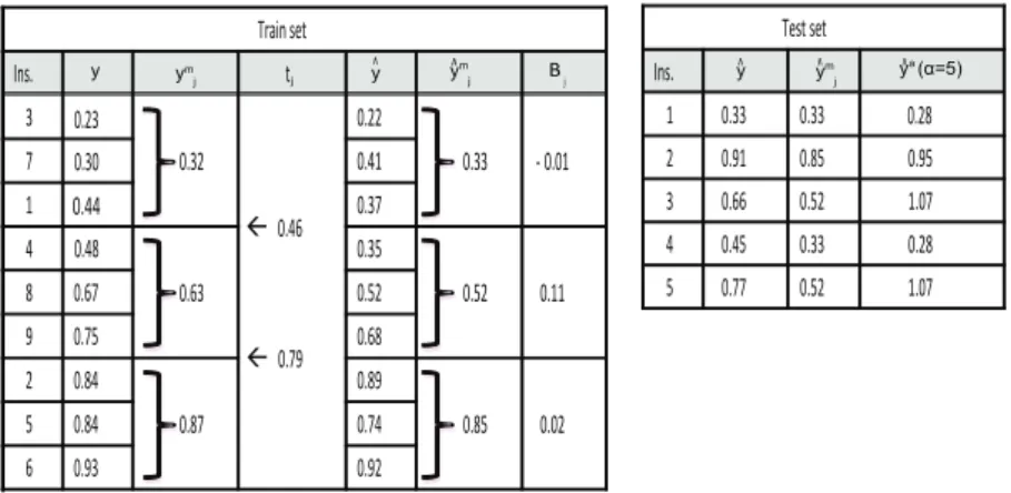
Figure 6 illustrates this process. On the training set (left) a segmentation method has generated three bins (with the same number of examples in each bin).The average values of each bin are,ym
1 = 0.32,ym2 = 0.63 andym3 = 0.87.
The threshold between the first and the second bin is t1 = 0.46, and the
threshold between the second and the third bin is t2 = 0.79. The estimated
average values for each bin are ˆym
1 = 0.33, ˆym2 = 0.52 and ˆy3m= 0.85. Therefore,
when the value predicted by the learning algorithm on the test set (right) for an instance is less than or equal to 0.46 the method assigns 0.33 to it. If the value predicted by the learning algorithm of an instance is between 0.46 and 0.79 the method assigns 0.52 to it. Finally, if the value is greater than 0.79 the method assigns 0.85. Clearly, segmentation does not provide enough granularity for instance regression, but here we are interested in quantification.
Fig. 6 Example of the predictions of a regression model for a test set (right) using the segmentation on the training set (left).On the left we show how the bins are constructed and how the biasBj is estimated for each bin using the differenceymj −ˆymj . On the right,
each example is assigned to a binj according to its prediction ˆy and the final adjusted prediction ˆyais given by Eq. 9 usingα= 5.
The example is also useful to see that segmentation has some effects on the distribution of the new output values. Segmentation makes prediction less sensitive to outliers and, depending on how the bins are chosen, the values might be more robust than a single prediction. In fact, it may have impor-tant and non-monotonic effects when the distribution is multimodal. Also, segmentation has the effect of reducing variability, especially ifk is small.
From this process, we can use the modified (segmented) predictions as the new numerical values for each example, which can be used for both RS
(Eq. 5 and 6) as seen in section 2.1. However, the interesting thing about the segmentation method comes when we combine it with an adjustment7, as justified by the third problem we have mentioned above: we cannot assume
7
Note that this adjustment is performed with information from the training data exclu-sively. An alternative possibility would be to use a validation dataset, but this would reduce the available training data.
that the bias Bj is the same for all the regions. So, instead of calculating a global adjustment as in Eq. 8, we calculate the bias for each bin in the training set, and we use it for the adjustment for that bin. In other words, we adjust each bin independently of the rest. This has much more impact on how predictions are modified, since some bins may have very poor estimated averages. As can be seen in Figure 6 we have calculated the meanyˆm
j of the predicted values ˆy on the training set of each binj, andBj is calculated for
each bin as (ym
j −yˆjm). From here, the adjusted value is calculated for each
instance in the test set as follows:
ˆ
ya = ˆymj +α·Bj (9)
In Figure 6 we consider α= 5, and we obtain 0.33 + 5·(−0.01) = 0.28 for example i = 1, 0.85 + 5·(0.11) = 0.95 for example i = 2 and so on. Note that many regression models will tend to issue predictions leaned towards the global average (because they are unsure on some cases and also becauseofthe
MSE penalisation, discussed in section 4.1). This will lead to different values ofBj for each bin, trying to set the values outwards.
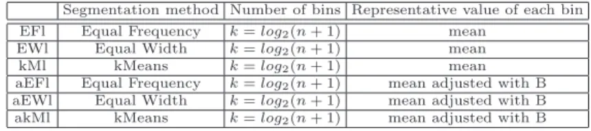
In order to apply the previous procedure, we need some segmentation meth-ods. Two methods will derive the segments using discretisation techniques and the third one will use a clustering method. The three of them will keep the numerical character of the output value (we are not discretising the prob-lem). Bakar et al. (Bakar et al, 2009) present an exhaustive taxonomy for data discretisation techniques. We will first explore two of the simplest and best-known unsupervised methods:Equal Frequency intervals(EF) andEqual Width intervals (EW) (Dougherty et al, 1995). Basically, these methods con-sist in sorting the values and splitting them in kbins. The number of bins is a parameter that has to be supplied by the user. EW puts the same num-ber of examples in each bin whereasEF creates bins with the same length: (max value−min value)/k. A third method (kM s) is not based on discreti-sation techniques and will segment the output values by usingk-means, which is one of the most popular clustering algorithms. Thek-means algorithm is ap-plied on the outputs, as in the other methods, so it finally creates a partition, which may be different to the other two cases.
All these three segmentation methods require a value for k. There are several formulae to automatically set the number of bins. For example, Sturges (Sturges, 1926) sets k = log2(n+ 1), where n is the number of instances. Yang (Yang, 2003) proposes a new discretisation method called Proportional Discretisation (P D) that combines the EF and EW methods. In P D, the number of examples in each bin (frequency) is equal to the number of bins, and the frequency multiplied by the number of bins is equal to the number of examples. Therefore, this method is equivalent to using theEF method with
k=√n. We have studied these two alternatives for establishingk. Since the results are quite similar for both options, in this paper we will only include the results for k = log2(n+ 1). For each segmentation method, we will also consider an unadjusted and an adjusted version. This leads to 6 combinations.