Model Development Of The Energy Demand By Utilizing Artificial Intelligence (AI) Technique

(1)

MODEL DEVELOPMENT OF THE ENERGY DEMAND BY UTILIZING ARTIFICIAL INTELLIGENCE (AI) TECHNIQUE

By

MUHAMMAD NASIH BIN SAIFULLAH

13732

FINAL PROJECT REPORT

Dissertation submitted in partial fulfilment of the requirement for the

Bachelor of Engineering (Hons) (Electrical and Electronic)

MAY 2014

Universiti Teknologi PETRONAS Bandar Seri Iskandar

31750 Tronoh

(2)

ii

CERTIFICATION OF APPROVAL

Model Development of the Energy Demand by Utilizing Artificial Intelligence (AI) Technique

By

Muhammad Nasih bin Saifullah 13732

A project dissertation submitted to the Electrical and Electronic Engineering Programme

Universiti Teknologi PETRONAS In partial fulfilment of the requirement for the

BACHELOR OF ENGINEERING (Hons) (ELECTRICAL AND ELECTRONIC)

Approved by,

________________________ (AP Dr. Zuhairi Hj Baharudin)

UNIVERSITI TEKNOLOGI PETRONAS

TRONOH, PERAK

(3)

iii

CERTIFICATION OF ORIGINALITY

This is to certify that I am responsible for the work submitted in this project, that the original work is my own except as specified in the references and acknowledgements, and that the original work contained herein have not been undertaken or done by unspecified sources or persons.

____________________________________ (MUHAMMAD NASIH BIN SAIFULLAH)

(4)

iv

ABSTRACT

Load forecasting has been one of the major researches in electrical engineering in the recent years. It plays a very important role in power system planning and operation. Through load forecasting, power generation can be balanced with load demand, which subsequently contributes to an efficient electricity management in power system. One way of forecasting load demand is by using Artificial Intelligence (AI) technique. There are two AI technique’s methods discussed in this project which are Artificial Neural Network (ANN) method and Fuzzy Logic (FL) method. Both approaches utilize MATLAB software. The accuracy of the forecast is based on the Mean Absolute Average Error (MAPE). Instead of using a year-long historical data, this project uses selective seasonal historical data, focusing on the autumn season. 1-hour ahead and 24-hour ahead load forecasts are developed for each approach. The first chapter of this report discusses the fundamental of each method and also statistical analysis of data. The following chapter describes how each method is developed by using MATLAB. Followed next is a chapter consisting of results of both models and followed by discussions of the results obtained. The last chapter is on conclusion as well as recommendations for any possible future continuation of the project.

(5)

v

ACKNOWLEDGEMENTS

I would like to thank my supervisor, AP Dr. Zuhairi Hj. Baharudin, an Associate Professor of Electrical and Electronic Engineering Department of Universiti Teknologi PETRONAS (UTP) for his guidance in completing this project. I would like to express an utmost gratitude to my parents as well for their endless support.

Besides that, my sincere appreciation goes to all my friends and those who have contributed either directly or indirectly in order to get this project completed.

(6)

vi

LIST OF FIGURES

Figure 1: Multilayer feedforward network architecture ... 5

Figure 2: Example showing correlation between linguistic variables of a membership function [27] ... 8

Figure 3: Triangular membership function of Fuzzy Logic method ... 8

Figure 4: Average load demand from March to May of 2006-2010 ... 10

Figure 5: Actual hourly load of the forecasted day ... 10

Figure 6: Development of Artificial Neural Network method ... 12

Figure 7: The structure of ANN model ... 13

Figure 8: Development of Fuzzy Logic method ... 14

Figure 9: Fuzzy system structure developed using MATLAB software ... 19

Figure 10: Actual load vs forecasted load for Monday ANN forecast ... 22

Figure 11: Actual load vs forecasted load for Tuesday ANN forecast ... 23

Figure 12: Actual vs forecasted load for Wednesday ANN forecast ... 23

Figure 13: Actual load vs forecasted load for Thursday ANN forecast ... 24

Figure 14: Actual load vs forecasted load for Friday ANN forecast ... 24

Figure 15: Actual load vs forecasted load for Saturday ANN forecast ... 25

Figure 16: Actual load vs forecasted load for Sunday ANN forecast ... 25

Figure 17: Actual load vs forecasted load for Monday Fuzzy Logic forecast ... 27

Figure 18: Actual load vs forecasted load for Tuesday Fuzzy Logic forecast ... 27

Figure 19: Actual load vs forecasted load for Wednesday Fuzzy Logic forecast ... 28

Figure 20: Actual load vs forecasted load for Thursday Fuzzy Logic forecast ... 28

Figure 21: Actual load vs forecasted load for Friday Fuzzy Logic forecast ... 29

Figure 22: Actual load vs forecasted load for Saturday Fuzzy Logic forecast ... 29

(9)

ix

LIST OF TABLES

Table 1: Monday’s membership functions data………15

Table 2: Tuesday’s membership functions data………...16

Table 3: Wednesday’s membership functions data………..16

Table 4: Thursday’s membership functions data………..17

Table 5: Friday’s membership functions data………..17

Table 6: Saturday’s membership functions data………..18

Table 7: Sunday’s membership functions data………18

Table 8: Fuzzy rules for Fuzzy Logic structure………...20

Table 9: Artificial Neural Network MAPEs………26

(10)

1

CHAPTER 1 INTRODUCTION

1.0 Background of Study

In load forecasting, there are three different categories which are short-term load forecasting (STLF), medium-term load forecasting (MTLF) and long-term load forecasting (LTLF) [1]. STLF refers to load forecasting from one hour to one week ahead of load occurrence while MTLF refers to load forecasting in a period within one week to one month ahead of load occurrence [2]. LTLF is usually for forecasting load demand for a period of more than one year [2] and used for planning operations [3].

The forecasting techniques that have been developed in the previous years could be categorized into three major groups [4]. They are traditional forecasting technique, modified traditional technique and also Artificial Intelligence (AI) technique.

The main objective of this project is to develop two load forecasting models to forecast the electric load demand of Australia using the data obtained from Australia Power Grid. The models that are to be developed are applying AI technique, where two approaches are used which are Artificial Neural Network (ANN) and Fuzzy Logic (FL).

(11)

2

1.1 Problem Statement

Forecasting energy demand, or specifically electric load demand plays a very important role in contributing to an efficient resource management. It helps to improve load factor and thus reduces energy wastage. Energy wastage occurs when the load demand is less than the power supplied. Energy wastage translates into a poor energy management, caused by high operating cost of the utilities through the handling of wastage surplus energy generated [5]. On the other hand, supplying electrical energy lower than demand also affects the system. Underprediction of load results in a failure to provide necessary reserves to meet the demand due to the expensive peaking units [5]. Hence, a reliable method of load forecasting is required to provide good forecast value of the future load demand.

1.2 Objectives

1. To study on Artificial Intelligence (AI) technique in developing the proposed short term load forecasting models.

2. To analyze and perform statistical analysis of the data.

3. To develop the proposed load forecasting models by using AI technique. 4. To provide an hour ahead and twenty-four hours ahead load forecast.

(12)

3

1.3 Scope of Study

The scope of work of this project includes understanding the principle of AI technique to forecast energy load demand. The project utilizes two AI technique’s approaches; Artificial Neural Network (ANN) and Fuzzy Logic (FL) – in developing the STLF models. The fundamentals, characteristics, and concept of each approach are studied to develop the models. Both ANN and FL approaches utilize MATLAB software. The proposed models will be simulated by using the data collected from Australia Power Grid, where statistical analysis on load patterns and load curves of the data is done thoroughly before they are used in simulating the models. Through the simulations, Mean Average Percentage Error (MAPE) is obtained and comparisons are made to justify which model would be more reliable with a higher accuracy for a STLF with 1-hour ahead duration and also 24-hour hour ahead duration.

(13)

4

CHAPTER 2 LITERATURE REVIEW

2.1 Artificial Neural Network

ANN is a mathematical model that mimics how the brain of a human being functions, specifically on pattern recognition and classification [6]. Just like the brain, this method has the capability to organize its neurons to perform complex calculations by adapting its surrounding environment [6], [7]. This special capability is one of the reasons why ANN is a widely accepted method in load forecasting since 1980. It gives better performances compared to other previous used techniques [8], [9] such as Regression Method, Autoregressive Moving-Average (ARMA) and Autoregressive Integrated Moving-Average (ARIMA) [4].

According to S. Haykin [6], in order to achieve a good performance in load forecast, neural networks employ a massive interconnection of neurons or could be called as processing units. Initially, the model goes through a repeated training with sequences of patterns on the past inputs and outputs. The training teaches the model to be able to forecast the output when only sequences of inputs are fed and it goes on until the network reaches a steady state. ANN reaches its steady state when there is no more significant changes in synaptic weights of the outputs [6], [10]. The learning process consumes quite some time and this has backfired the model because it is incapable of adopting sudden and rapid fluctuations in input variables like temperature.

(14)

5

2.1.1 Network Architecture

In general, there are three architectures for ANN [11]:

i. Single Layer Feed-forward Network; ii. Multilayer Feed-Forward Network; and iii. Recurrent Network

Each type of network differs in terms of the numbers of weighted interconnection layer, numbers of hidden layer and the presence of feedback loops.

This project employs multilayer feed-forward network architecture in developing ANN model to forecast the energy demand. The selected architecture consists of a single input layer, several hidden layers and one output layer where each layer could be of multiple neurons. Signal propagation between nodes within the same layer and from input nodes direct to outputs nodes are prohibited [12]. Hidden layers would help the signal propagation from input layer to output layer. The number of hidden layers and nodes per layer are problem dependent. Figure 1 below shows the multilayer feed-forward network architecture [12], [13]:

(15)

6

2.1.2 Learning Paradigm

In regards of neural network modelling, learning means the process of adapting its free parameters through a process of stimulation by the environment where the network is embedded [6] and changes accordingly. Through the changes that network has undergone in its internal structure, the network would then responds in a new way to its surrounding. With two different learning paradigms; unsupervised learning and supervised learning – comes five learning algorithms.

The learning algorithm that this project implements is Levenberg-Marquadt back-propagation learning algorithm. This algorithm takes the input, passes them through hidden layers and gives results of calculation through the output layer [14]. Appropriate mappings are done throughout the learning process and adjustment on the weights and biases at each iteration of the mappings are made to improve the output [15].

Levenberg-Marquadt back-propagation algorithm uses an approximation of Newton’s method, which contains approximation of Hessian matrix and Jacobian matrix [9]. This algorithm is chosen among other activation functions such as steepest descent propagation (SDBP) and momentum back-propagation (MBP). It yields a speed-up of large factors via limited modifications of the standard back-propagation algorithm and hence gives faster convergence rate [16], [17].

2.2 Fuzzy Logic

While ANN learns through its surrounding, FL provides a mean for representing uncertainties through a mapping done by a number of if-then rules [18], [19]. This approach has advantages over ANN because it could deal with non-linear parts of the forecasted load curves and also with the abrupt changes in the variables such as the temperature of the day [20], [21], [22].

(16)

7

2.2.1 Fuzzy Sets

A fuzzy set contains a classical set without crisp that wholly includes or wholly exclude any given elements. Taking an example of element X and Y, X and Y must either be in a set named A or in set not-A. The sets are called linguistic variables such as hot, very hot, mild, high and small.

For example, the temperature inputs are translated into low temperature, medium temperature and high temperature in fuzzification process. This mapping permits the incorporation of the expert knowledge, which is represented by the descriptive natural language with the FL model [23], [24]. Since the description of linguistic terms used is very relative, the covered range of each membership function needs to be defined [25]. The range, termed as the universe of discourse [26] is normalized between 0 and 1.

2.2.2 Membership Functions

A membership function, or called as a degree of ‘belonging’ [26] is a curve to define how each input is mapped to its respective degree of membership between the values 0 to 1. Fuzzy sets only describe the basic concepts or information of the inputs by assigning linguistic languages and hence admits the possibility of partial membership in it. These input values are then associated with a membership function to their respective membership value to further distinguish an input to the other inputs in FL model.

In associating linguistic variables to each other, as shown in the figure below, the interception point between the two linguistic variables at 0 indicates non-member meanwhile 1 indicates full non-member of the non-membership function [25].

(17)

8

Figure 2: Example showing correlation between linguistic variables of a membership function [27]

Each variable has varying degrees of membership. There are several methods that can be used to derive each membership function. It can be based on intuition, expert knowledge on the variable, subjective judgment or interpolation of the actual data.

The type of membership function used in this project is triangular membership function, as depicted in the figure below.

Figure 3: Triangular membership function of Fuzzy Logic method

2.2.3 Basic Configuration

The basic configuration of FL system [18], [28] is divided into four elements:

2.2.3.1 Fuzzification

(18)

9

2.2.3.2 Fuzzy rule base

A set of conditional statements formed using if-then statements. Fuzzy rules are formulated subjectively which can be based on intuition or expert knowledge.

2.2.3.3 Fuzzy inference engine

It consists of the if-then statements developed in fuzzy rule base. It is a mapping process of fuzzy inputs to the fuzzy outputs based on the fuzzy rules and fuzzy set database. This process provides the decision making logic of the developed model. An example rule to further describe the IF … THEN statement rules of the system is as followed:

If ‘temperature is high’ and ‘humidity is medium’, then ‘the load demand is high’.

2.2.3.4 Defuzzification interface

A process of defuzzifying the fuzzy outputs to generate non-fuzzy outputs.

FL model adopts the use of linguistic languages of explanatory variables in modelling the approach. More explanatory variables such as classification of the previous day as a holiday or not can be introduced. More variables do not necessarily mean better result. Conflicts of input-output pairs prompt to happen frequently because the input variables are mapped to a few different functions [29].

2.3 Data Analysis

This project focuses on investigating the effect of seasonal load data on the forecasting instead of year-long hourly data. Autumn season is selected for this purpose. Therefore, the historical data consists of hourly load demand for each day from March until May for the year 2006 to 2010 are used.

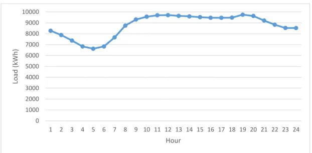
Figure 4 below is a graph depicting the hourly average load demand of the Australia Grid for the specified data set. The lowest load demand is observed to between the 3rd hour (HR0200) and 8th hour (HR0700) while high load demand is between 12th hour (HR1100) and 20th hour (HR1900).

(19)

10

Figure 4: Average load demand from March to May of 2006-2010

All the forecasted load demands obtained from both ANN and FL methods are compared to the actual hourly load data. The actual load demand of each day are presented in the figure below.

Figure 5: Actual hourly load of the forecasted day

0 1000 2000 3000 4000 5000 6000 7000 8000 9000 10000 1 2 3 4 5 6 7 8 9 10 11 12 13 14 15 16 17 18 19 20 21 22 23 24 Lo ad (k Wh ) Hour 0 2000 4000 6000 8000 10000 12000 1 2 3 4 5 6 7 8 9 10 11 12 13 14 15 16 17 18 19 20 21 22 23 24 Lo ad (k Wh ) Hour

Monday Tuesday Wednesday Thursday

(20)

11

CHAPTER 3 METHODOLOGY

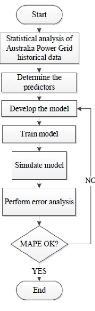
To achieve the stated objectives, a preliminary research is done to understand the techniques used in forecasting load demand. The primary focus of the research is on AI technique. Next, the fundamentals of software to be utilized in this project are studied. Both ANN and FL approaches utilize MATLAB software. The models that are developed in this project uses data from Australia Power Grid. Statistical analysis is performed to understand the patterns of the historical load demand of Australia Power Grid.

The next stage involves the development of ANN and FL models by employing MATLAB software. These models are then trained with sample data to forecast 1-hour ahead and 24-hour ahead load forecast. Subsequent needed adjustments to the models are carried out to get more accurate forecast. Once the training gives a satisfactory results, the models are simulated with data and outputs are calculated. Troubleshoots on the models are carried out if the Mean Absolute Percentage Error (MAPE) produced is not satisfactory.

The project utilizes Australia Power Grid Data for year 2006 to 2010. Instead of using year-long historical data, a selective range of data has been used for developing the models. This project aims to provide seasonal load forecast. Hence, only historical data for autumn season are used.

MAPE for both models are calculated based on the following formula:

𝑀𝐴𝑃𝐸 =1 𝑛∑ | 𝐴_𝑡− 𝐹_𝑡 𝐴_𝑡 | 𝑛 𝑡=1 𝑥 100%

(21)

12

3.1 Artificial Neural Network

Figure 11 summarizes the stages and processes involved in the project for ANN method.

Figure 6: Development of Artificial Neural Network method

In ANN method, the data go through multiple processes in producing the forecasted output. There are three processes and they are called data treatment.

3.1.1 Data Arrangement

The data are arranged so that the model can recognize the sequence of the data fed into the model. The model recognizes the data according to the hourly sequence, day sequence, month sequence and year sequence respectively.

(22)

13

3.1.2 Data Normalization

In input neurons, the input model use transfer function of tansig. Therefore, the data range development that can be used in the model is from -1 to +1. The data are then normalized by dividing the input by 10000 and converted back to their actual value by the same integer once the model have produced the needed forecast value. The idea of normalizing the data is to avoid lagging of data processing in MATLAB software.

3.1.3 Data Partitioning

With a total 1152 samples are available, 70% of the samples are used for training and the remaining 30% are used for validation purpose.

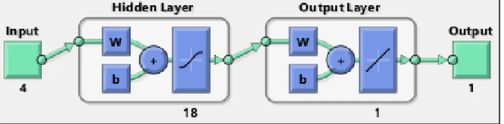
Figure 7: The structure of ANN model

The model takes 4 predictors as input variables. The inputs of the ANN method classed into the following predictors:

1. The hour of the day 2. The month of the day

3. Previous weeks’ same hour load 4. Yesterday’s same hour load

The hidden layer contains 18 neurons. Multiple simulations with the tested number of neurons ranging from 5 to 28 are run to obtain an optimum number while maintaining the same 70:30 training and testing ratio.

(23)

14

3.2 Fuzzy Logic

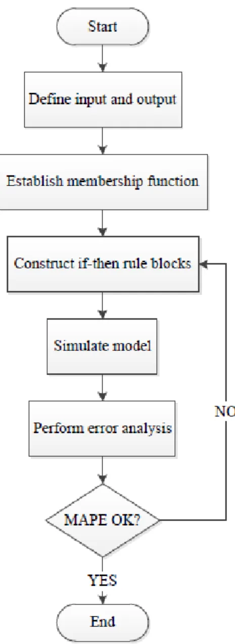
The overall development of FL method [18] is described in the figure below.

Figure 8: Development of Fuzzy Logic method

There are 2 factors used in the model to forecast the next day load demand. They are load and temperature. Temperature is an important factor because the load can be high when the temperature is high and the load can be low when the temperature is low.

Apart from temperature, another factor considered is load. In this project, the FL model utilizes the previous weeks same day load and yesterday’s load. The previous week same day load contributes a weightage in terms of the typical load demand of the particular day. The previous day load is also considered to influence to next day load

(24)

15

because it contributes a weightage in providing the system the expected range of load demand of the next day.

The following statistical analysis approach is used to identify the membership functions. The maximum and minimum load, quartile 1, quartile 2, quartile 3 and mean of previous weeks same day load, yesterday’s load and yesterday’s temperature are calculated.

The model uses the hourly previous weeks same day load and hourly yesterday’s load. Therefore, the total data sample, n = 24 x 2 = 48.

The quartiles are formulated by using the following formulas:

𝑄𝑢𝑎𝑟𝑡𝑖𝑙𝑒 1 = 𝑛 + 1 4 𝑄𝑢𝑎𝑟𝑡𝑖𝑙𝑒 2 = 𝑛 + 2 4 𝑄𝑢𝑎𝑟𝑡𝑖𝑙𝑒 3 = 𝑛 + 3 4

By using the values obtained through the formulas above to set the upper and lower bounds of each membership function’s range, the four triangular membership functions of each day are developed. As each day’s load data is different, a different set of membership functions are developed for each day.

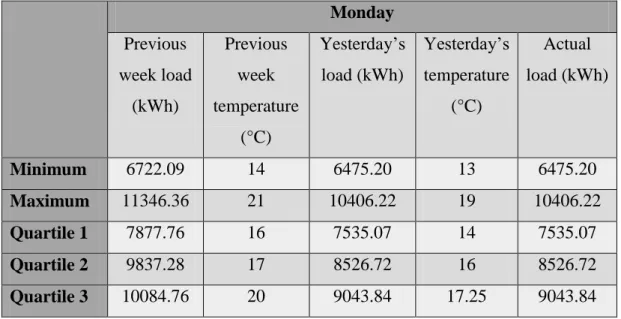
Table 1: Monday's membership functions data

Monday Previous week load (kWh) Previous week temperature (°C) Yesterday’s load (kWh) Yesterday’s temperature (°C) Actual load (kWh) Minimum 6722.09 14 6475.20 13 6475.20 Maximum 11346.36 21 10406.22 19 10406.22 Quartile 1 7877.76 16 7535.07 14 7535.07 Quartile 2 9837.28 17 8526.72 16 8526.72 Quartile 3 10084.76 20 9043.84 17.25 9043.84

(25)

16

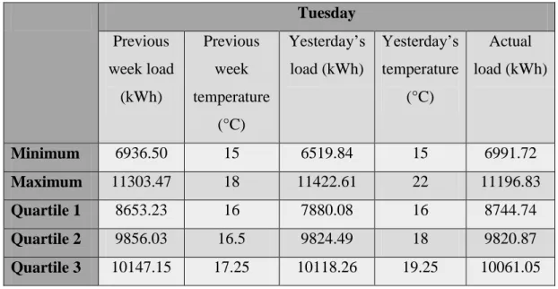
Table 2: Tuesday's membership functions data

Tuesday Previous week load (kWh) Previous week temperature (°C) Yesterday’s load (kWh) Yesterday’s temperature (°C) Actual load (kWh) Minimum 6936.50 15 6519.84 15 6991.72 Maximum 11303.47 18 11422.61 22 11196.83 Quartile 1 8653.23 16 7880.08 16 8744.74 Quartile 2 9856.03 16.5 9824.49 18 9820.87 Quartile 3 10147.15 17.25 10118.26 19.25 10061.05

Table 3: Wednesday's membership functions data

Wednesday Previous week load (kWh) Previous week temperature (°C) Yesterday’s load (kWh) Yesterday’s temperature (°C) Actual load (kWh) Minimum 7038.08 15 6991.72 15 6790.27 Maximum 10968.15 19 11196.83 19 11422.97 Quartile 1 8852.29 15.5 8744.74 15.5 8169.17 Quartile 2 9475.37 16 9820.87 17 9817.36 Quartile 3 9978.71 18 10061.05 18.25 10306.01

(26)

17

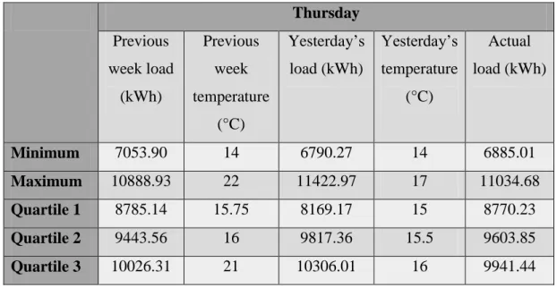
Table 4: Thursday's membership functions data

Thursday Previous week load (kWh) Previous week temperature (°C) Yesterday’s load (kWh) Yesterday’s temperature (°C) Actual load (kWh) Minimum 7053.90 14 6790.27 14 6885.01 Maximum 10888.93 22 11422.97 17 11034.68 Quartile 1 8785.14 15.75 8169.17 15 8770.23 Quartile 2 9443.56 16 9817.36 15.5 9603.85 Quartile 3 10026.31 21 10306.01 16 9941.44

Table 5: Friday's membership functions data

Friday Previous week load (kWh) Previous week temperature (°C) Yesterday’s load (kWh) Yesterday’s temperature (°C) Actual load (kWh) Minimum 7021.20 13 6885.01 16 6897.19 Maximum 10633.79 21 11034.68 19 10598.60 Quartile 1 8797.61 15 8770.23 16.5 8884.55 Quartile 2 9509.92 15.5 9603.85 18 9478.36 Quartile 3 9883.90 19 9941.44 19 9862.08

(27)

18

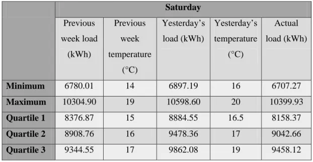
Table 6: Saturday's membership functions data

Saturday Previous week load (kWh) Previous week temperature (°C) Yesterday’s load (kWh) Yesterday’s temperature (°C) Actual load (kWh) Minimum 6780.01 14 6897.19 16 6707.27 Maximum 10304.90 19 10598.60 20 10399.93 Quartile 1 8376.87 15 8884.55 16.5 8158.37 Quartile 2 8908.76 16 9478.36 17 9042.66 Quartile 3 9344.55 17 9862.08 19 9458.12

Table 7: Sunday's membership functions data

Sunday Previous week load (kWh) Previous week temperature (°C) Yesterday’s load (kWh) Yesterday’s temperature (°C) Actual load (kWh) Minimum 6713.14 14 6707.27 13 6475.20 Maximum 10520.49 20 10399.93 23 10406.22 Quartile 1 7913.02 15 8158.37 15 7535.07 Quartile 2 8894.08 16 9042.66 15.5 8526.72 Quartile 3 9348.73 17.5 9458.12 18.5 9043.84

Based on the membership functions developed using the above data, a fuzzy system structure as depicted in the figure below is developed. The same structure is used for each day.

(28)

19

Figure 9: Fuzzy system structure developed using MATLAB software

With all fuzzy parameters ready, fuzzy rules are developed. Table 8 lists all the fuzzy rules used in this fuzzy system model. Even though each day has different structure due to different range of parameters developed based on the statistical analysis above, each structure has the same fuzzy rules.

(29)

20

Table 8: Fuzzy rules for Fuzzy Logic structure

Previous week load Previous week temperature Previous day load Previous day temperature Forecast

Very low Very low Very low Very low Very low

Very low Low Very low Very low Very low

Very low Very low Very low Low Very low

Very low Low Very low Low Very low

Low Low Low Low Low

Low Very low Low Low Low

Low Low Low Very low Low

Low Very low Very low Very low Very low

Low Very low Very low Low Low

Medium Low Medium Low Medium

Medium Low High Low medium

Medium Very low Low Low Low

Medium Very low Medium Low Medium

Medium High Medium High Medium

Medium Very high Medium High Medium

Medium High Medium Very high Medium

High Very high High High High

High High High High High

High Medium High Medium High

High Low High Medium High

High Very low High Medium Medium

High Medium Low Low high

Very high High Very high Very high Very high

(30)

21

3.3 Gantt Chart

3.4 Key Milestones

A few key milestones are set to accomplish the objectives of this project:

1 2 3 4 5 6 7 8 9 10111213141516171819202122232425262728

Proposal of topic title Preliminary research of the topic Obtaining data Statistical analysis of data Development of models Simulation of models Documentation

(31)

22

CHAPTER 4 RESULTS AND DISCUSSION

4.1 Artificial Neural Network

In this project, historical data of every Friday from March to May for the year 2006 until 2010 are used as predictors for the training. These predictors are used to train the model that has been developed. Once the model is ready, 1-hour ahead and 24-hour ahead load forecasts of the next Friday are carried out.

Figure 10 to Figure 16 show the forecasted load against the actual load for 1-hour ahead and 24-hour ahead forecasts for each day. The table that follows tabulate the MAPEs recorded for ANN model.

Figure 10: Actual load vs forecasted load for Monday ANN forecast

0 2000 4000 6000 8000 10000 12000 1 2 3 4 5 6 7 8 9 10 11 12 13 14 15 16 17 18 19 20 21 22 23 24 Lo ad ( kWh ) Hour

(32)

23

Figure 11: Actual load vs forecasted load for Tuesday ANN forecast

Figure 12: Actual vs forecasted load for Wednesday ANN forecast

0 2000 4000 6000 8000 10000 12000 1 2 3 4 5 6 7 8 9 10 11 12 13 14 15 16 17 18 19 20 21 22 23 24 Lo ad ( kWh ) Hour

Actual 1-hour ahead 24-hour ahead

0 2000 4000 6000 8000 10000 12000 1 2 3 4 5 6 7 8 9 10 11 12 13 14 15 16 17 18 19 20 21 22 23 24 Lo ad ( kWh ) Hour

(33)

24

Figure 13: Actual load vs forecasted load for Thursday ANN forecast

Figure 14: Actual load vs forecasted load for Friday ANN forecast

0 2000 4000 6000 8000 10000 12000 1 2 3 4 5 6 7 8 9 10 11 12 13 14 15 16 17 18 19 20 21 22 23 24 Lo ad ( kWh ) Hour

(34)

25

Figure 15: Actual load vs forecasted load for Saturday ANN forecast

Figure 16: Actual load vs forecasted load for Sunday ANN forecast

0 2000 4000 6000 8000 10000 12000 1 2 3 4 5 6 7 8 9 10 11 12 13 14 15 16 17 18 19 20 21 22 23 24 Lo ad ( kWh ) Hour

(35)

26

Table 9: Artificial Neural Network MAPEs

Day

MAPE (%)

1-hour ahead 24-hour ahead

Monday 1.939 2.376 Tuesday 1.526 2.544 Wednesday 2.897 3.025 Thursday 1.527 1.647 Friday 1.680 2.705 Saturday 2.861 3.617 Sunday 2.806 2.840 Average MAPE (%) 2.177 2.679

It is observed that by using seasonal load data, the MAPE obtained for both forecasts range between 2.1% and 2.7% where 1-hour ahead forecast gives better accuracy than 24-hour ahead forecast. Higher MAPEs are recorded for Wednesday, Saturday and Sunday. The average MAPE calculated in this ANN model represents the average MAPE for all 7 days without separating the days into weekends and weekdays.

1-hour ahead forecast utilizes the actual previous same hour load to forecast the next hour load. Meanwhile, 24-hour ahead forecast also includes the forecasted load of the previous hour load in forecasting the next hour load. This is one of the factors that leads to the poorer accuracy of 24-hour ahead forecast as compared to 1-hour ahead forecast.

(36)

27

4.2 Fuzzy Logic

Figure 17 to Figure 23 compare the actual load against the forecasted load using FL method for both 1-hour ahead and 24-hour ahead forecasts. Meanwhile, the MAPEs of all 7 days are tabulated in the table that follows.

Figure 17: Actual load vs forecasted load for Monday Fuzzy Logic forecast

Figure 18: Actual load vs forecasted load for Tuesday Fuzzy Logic forecast

0 2000 4000 6000 8000 10000 12000 1 2 3 4 5 6 7 8 9 10 11 12 13 14 15 16 17 18 19 20 21 22 23 24 Lo ad ( kW h ) Hour

Actual load FL 1-hour ahead FL 24-hour ahead

0 2000 4000 6000 8000 10000 12000 1 2 3 4 5 6 7 8 9 10 11 12 13 14 15 16 17 18 19 20 21 22 23 24 Lo ad ( kWh ) Hour

(37)

28

Figure 19: Actual load vs forecasted load for Wednesday Fuzzy Logic forecast

Figure 20: Actual load vs forecasted load for Thursday Fuzzy Logic forecast

0 2000 4000 6000 8000 10000 12000 1 2 3 4 5 6 7 8 9 10 11 12 13 14 15 16 17 18 19 20 21 22 23 24 Lo ad ( kWh ) Hour

(38)

29

Figure 21: Actual load vs forecasted load for Friday Fuzzy Logic forecast

Figure 22: Actual load vs forecasted load for Saturday Fuzzy Logic forecast

0 2000 4000 6000 8000 10000 12000 1 2 3 4 5 6 7 8 9 10 11 12 13 14 15 16 17 18 19 20 21 22 23 24 Lo ad ( kWh ) Hour

(39)

30

Figure 23: Actual load vs forecasted load for Sunday Fuzzy Logic forecast

Table 10: Fuzzy Logic MAPEs

Day

MAPE (%)

1-hour ahead 24-hour ahead

Monday 4.250 5.454 Tuesday 4.934 5.402 Wednesday 4.001 5.398 Thursday 8.008 8.406 Friday 5.376 5.778 Saturday 4.166 4.858 Sunday 6.258 7.321 Average MAPE (%) 5.285 6.088

The average MAPE obtained for FL 1-hour ahead forecast is 5.285% while FL 24-hour ahead forecast records an average MAPE of 6.088%. These high MAPEs recorded for FL method are contributed by a few factors.

0 2000 4000 6000 8000 10000 12000 1 2 3 4 5 6 7 8 9 10 11 12 13 14 15 16 17 18 19 20 21 22 23 24 Lo ad ( kWh ) Hour

(40)

31

The FL method developed in this project utilizes the data of previous week and yesterday’s load as well as previous week and yesterday’s temperature. The results suggest that there might not be important correlation between the past 24 hours load and the current load.

There are other factors like festive days and public holidays that might contribute to the hourly load demand. In addition, although each day’s system structure has different range of temperature and load, each system structure has been developed based on the same fuzzy rules.

(41)

32

CHAPTER 5 CONCLUSION AND RECOMMENDATION

5.1 Conclusion

Artificial Neural Network (ANN) model is developed by establishing a functional system aimed for data error detection. The model investigates a number of parameters which include learning algorithm, activation function, the training of input variables, data validation and the number of neurons used. On the other hand, Fuzzy Logic (FL) model is developed based on the non-linear variables. Apart from statistical analysis, the model can also be developed by intuitive judgments or expert knowledge.

This project has been able to develop both ANN and FL approaches. Both approaches are developed to forecast hourly load demand categorized by day. For ANN approach, the average MAPE obtained for 1-hour ahead and 24-ahead forecasts is 2.177% and 2.679% respectively. On the other hand, FL method has recorded an average MAPE of 5.285% and 6.088% for 1-hour ahead and 24-hour ahead forecast respectively.

MAPE represents the accuracy of the forecast to the actual load. Lower MAPE means better model. In this project, the FL model that has been developed has achieved a satisfactory MAPE yet unreliable to be used in industry.

Between the two approaches that have been developed in this project, ANN proves to a better model with a better MAPE. 1-hour ahead load forecast is more accurate than 24-hour load forecast for both models.

(42)

33

5.2 Recommendation

There are some other parameters that can be included in both models for future development in order to produce a better forecast. The average of the hourly load can be included to give better forecast result. Besides that, the factor of festive days or public holidays can also be made as one of the variables.

For FL approach, further investigation can be made on the model by applying different set of fuzzy rules for each day’s system structure. Each day’s structure has different membership function range and varied quartile values. Hence, the correlation between each fuzzy set of each day will differ.

Apart from just 1-hour and 24-hour ahead load forecasts, a 12-hour load forecast can also be considered to be developed if there is any future continuation on the project.

(43)

34

References

[1] H. E.-Z. I. Badran, G. Halasa, "Short-Term and Medium-Term Load Forecasting for Jordan's Power System," American Journal of Applied

Sciences, pp. 763-768, 2008.

[2] G. Gross and F. D. Galiana, "Short-term load forecasting," Proceedings of the

IEEE, vol. 75, pp. 1558-1573, 1987.

[3] M. F. Irzaq bin Khamis, Z. bin Baharudin, N. Hisham bin Hamid, M. F. bin Abdullah, and S. S. M. Yunus, "Electricity forecasting for small scale power system using fuzzy logic," in IPEC, 2010 Conference Proceedings, 2010, pp. 1040-1045.

[4] A. K. Singh, I. Ibraheem, S. Khatoon, M. Muazzam, and D. K. Chaturvedi, "Load forecasting techniques and methodologies: A review," in Power, Control and Embedded Systems (ICPCES), 2012 2nd International Conference on, 2012, pp. 1-10.

[5] A. G. Bakirtzis, V. Petridis, S. J. Kiartzis, M. C. Alexiadis, and A. H. Maissis, "A neural network short term load forecasting model for the Greek power system," Power Systems, IEEE Transactions on, vol. 11, pp. 858-863, 1996. [6] S. Haykin, Neural Networks: A Comprehensive Foundation. New Jersey:

Prentice-Hall, 1999.

[7] T. Senjyu, H. Takara, K. Uezato, and T. Funabashi, "One-hour-ahead load forecasting using neural network," Power Systems, IEEE Transactions on, vol. 17, pp. 113-118, 2002.

[8] M. Q. Raza and Z. Baharudin, "A review on short term load forecasting using hybrid neural network techniques," in Power and Energy (PECon), 2012 IEEE

International Conference on, 2012, pp. 846-851.

[9] T. Chin Yen, J. B. Cardell, and G. W. Ellis, "Short-term load forecasting using artificial neural networks," in North American Power Symposium (NAPS), 2009, 2009, pp. 1-6.

[10] K. B. Sahay and M. M. Tripathi, "Day ahead hourly load and price forecast in ISO New England market using ANN," in India Conference (INDICON), 2013

(44)

35

[11] M. M. Faiz, "Neural Network Application to Short Term Load Forecast," Bachelor of Engineering (Hons), Electrical & Electronics Engineering, Universiti Teknologi PETRONAS, Tronoh, 2012.

[12] Y.-Y. Hsu and Y. Chien-Chuen, "Design of artificial neural networks for short-term load forecasting. II. Multilayer feedforward networks for peak load and valley load forecasting," Generation, Transmission and Distribution, IEE

Proceedings C, vol. 138, pp. 414-418, 1991.

[13] H. S. Hippert, C. E. Pedreira, and R. C. Souza, "Neural networks for short-term load forecasting: a review and evaluation," Power Systems, IEEE Transactions on, vol. 16, pp. 44-55, 2001.

[14] A. F. Hasbullah, "Neural Network with Genetic Algorithm Prediction Model of Energy Consumption for Billing Integrity in Gas Pipeline," Electrical and Electronic Engineering, Universiti Teknologi PETRONAS, Tronoh, 2012. [15] J. P. S. Catalão, S. J. P. S. Mariano, V. M. F. Mendes, and L. A. F. M. Ferreira,

"Short-term electricity prices forecasting in a competitive market: A neural network approach," Electric Power Systems Research, vol. 77, pp. 1297-1304, 8// 2007.

[16] L. M. Saini and M. K. Soni, "Artificial neural network based peak load forecasting using Levenberg-Marquardt and quasi-Newton methods,"

Generation, Transmission and Distribution, IEE Proceedings-, vol. 149, pp.

578-584, 2002.

[17] L. Mohan Saini and M. K. Soni, "Artificial neural network-based peak load forecasting using conjugate gradient methods," Power Systems, IEEE

Transactions on, vol. 17, pp. 907-912, 2002.

[18] M. F. I. Khamis, Z. Baharudin, N. H. Hamid, M. F. Abdullah, and F. T. Nordin, "Short term load forecasting for small scale power system using fuzzy logic,"

in Modeling, Simulation and Applied Optimization (ICMSAO), 2011 4th

International Conference on, 2011.

[19] S. B. Ahmadi, H.; Jannaty H., "A fuzzy inference model for short-term load forecasting," presented at the 2012 Second Iranian Conference on Renewable Energy and Distributed Generation, 2012.

[20] A. J. E. Srinivas, "A Methodology for Short Term Load Forecasting Using Fuzzy Logic and Similarity," in The National Conference on Advances in

(45)

36

Computational Intelligence Applications in Power, Control, Signal Processing

and Telecommunications, Bhubaneswar, India, 2009.

[21] T. Senjyu, P. Mandal, K. Uezato, and T. Funabashi, "Next day load curve forecasting using hybrid correction method," Power Systems, IEEE

Transactions on, vol. 20, pp. 102-109, 2005.

[22] N. Farah, M. T. Khadir, I. Bouaziz, and H. Kennouche, "Short-term forecasting of Algerian load using fuzzy logic and expert system," in Multimedia

Computing and Systems, 2009. ICMCS '09. International Conference on, 2009,

pp. 81-86.

[23] S. Chenthur Pandian, K. Duraiswamy, C. Christober Asir Rajan, and N. Kanagaraj, "Fuzzy approach for short term load forecasting," Electric Power

Systems Research, vol. 76, pp. 541-548, 4// 2006.

[24] Z. Ismail, Mansor, R., "Fuzzy Logic Approach for Forecasting Half-hourly Malaysia Electricity Load Demand," in International Symposium on

Forecasting, 2011.

[25] C. Mo-Yuen and H. Tram, "Application of fuzzy logic technology for spatial load forecasting," Power Systems, IEEE Transactions on, vol. 12, pp. 1360-1366, 1997.

[26] T. R. Lonergan, J.V, "Linguistic Modelling of Short-Timescale Electricity Consumption Using Fuzzy Modelling Techniques," 2011.

[27] P. Patel, ed.

[28] W. Ma, X. Bai, and L. Mu, "Short-term load forecasting with artificial neural network and fuzzy logic," in Power System Technology, 2002. Proceedings.

PowerCon 2002. International Conference on, 2002, pp. 1101-1104 vol.2.

[29] D. K. Ranaweera, N. F. Hubele, and G. G. Karady, "Fuzzy logic for short term load forecasting," International Journal of Electrical Power & Energy