Autonomous navigation with deadlock detection
and avoidance
Sanchez, Guido1,2 and Giovanini, Leonardo1,2
1
Center for Signals, Systems and Computational Intelligence, Faculty of Engineering and Water Sciences, Universidad Nacional del Litoral
2 National Council for Scientific and Technological Research
Abstract. This paper studies alternatives to solve the problem of au-tonomous mobile robots navigation in unknown indoor environments. The navigation system uses fuzzy logic to combine the information ob-tained from range sensors and the navigational data to plan the robot’s movements. The strategy is built upon five modules:i)target following,
ii)obstacle avoidance, iii) possible path,iv) deadlock detection andv)
wall following. Given a possible path and obstacles near the environment of the robot, the controller will modulate the output velocity in order to go to the target and avoid collisions. In case of dead lock situations, a method that enables the robot to detect, escape and reach the target is proposed. The performance and behavior of the proposed navigational system was evaluated through simulations in different conditions, where the effectiveness of the proposed method is demonstrated and compared with previous results.
1
Introduction
One of the main objectives in mobile robotics is the design of autonomous robots: robots that can be told what to do without having to tell them how to do it. A major challenge faced by such robots is to make sure that their actions are executed correctly and reliably, despite the dynamics and inherent uncertainty of the working space.
A possible solution to this problem is to combine both path planning and path tracking, this approach is known asmotion planning with complete information. This method requires to know the environment before the motion starts and then the algorithm transforms this information into proper motion trajectories. Li et al. [8] uses a genetic algorithm for optimum path planning, focusing on the shortest distance criterion. Several other optimization methods have been developed to solve the optimum path-planning problem [4, 7, 12, 15, 21]. While this approach is well suited for structured environments, cannot be used in any real world situations, mainly because sometimes objects cannot be described or because one doesn’t know which object is going to be where and when.
If the robot has to move in an environment that is not predesigned and/or has no complete prior information, we are in the scope ofmotion planning with incomplete information. In this case, the robot must use real-time sensing and
sensor data processing to gather information about the surroundings. Generally, the robot moves reacting to obstacles while trying to get to the target. Typical examples of these techniques include potential-field methods [3] and fuzzy ap-proaches [1, 2, 5, 16, 17, 19, 20]. Because the source of information is mainly local, these methods have the drawback that are prone to get trapped in deadlock situations [1, 2, 16, 17] and because of this, particular attention is paid to the deadlock problem.
When the robot is in a deadlock situation –also called local minima, limit cycle orinfinite loop–, it will repeat indefinitely the same trajectory unless this is detected. This problem has been addressed using three types of approach: i) the boundary-following approach [1], ii) the virtual subgoal approach [18, 19] and iii) the behavior integration approach [10, 16]. Boundary-following ap-proaches generally detect a deadlock when the robot makes a sharp turn or when all sensors detect short obstacle distances. Then, the robot follows the bound-ary of the obstacle until an escape criterion is satisfied. This strategy can get trapped following a boundary indefinitely if the escape criterion fails to activate and may lead to rather inefficient paths because there is no way to choose the right boundary-following direction. Virtual subgoal approaches typically detect a deadlock whenever the robot makes a sharp turn or when the robot visits the same location more than one time. Then, the robot generates a new subgoal to escape the deadlock and returns the original goal when an escape criterion is satisfied. These methods may overproduce virtual subgoals leading to a dead-lock arising from conflictive subgoals. Behavior integration approaches usually make a map that models the surroundings of the robot, while a planning and a reactive module suggest a direction to escape from the deadlock and a direc-tion that avoids obstacles, respectively. These behaviors are then integrated to drive the robot to the goal. Building a map of the traversed path may be an issue when the system requires low memory and processing capabilities, like a microcontroller or a small computer.
In this paper we develop an autonomous navigation system for mobile robots in unknown environments, where the robot must be capable to go from a starting point A to a target point B. The information available to the robot is limited to its own position and those of the starting point A and target point B. Also, the robot is capable of detecting its own distance to obstacles. This information should be sufficient to reach the objective position. The proposed navigation system was developed using fuzzy logic, which has proved to be an appropriate tool to design robust systems in presence of noise [5, 14, 19] and signal processing tools [13] for detecting the deadlock situation.
In an attempt to meet these objectives, we make the following restrictions: i) we consider the navigation of a single mobile robot, ii) the robot does not generate maps of the traversed path, andiii)the environment is assumed to be a flat indoor environments without slippage between the wheels of the robot and the floor.
The main contribution of this article is a procedure for the identification of the deadlock situation during the robot’s traversal. The proposed method uses
only the distance to the target dtand the autocorrelation function to detect if
the robot is in a deadlock. Once a deadlock situation is detected, a wall-following behavior makes the robot escape from the deadlock.
The organization of the article is as follows. Section 2 presents the system configuration. Section 3 describes the fuzzy based navigation system and Sub-section 3.4 describes the deadlock detection and avoidance strategy. Section 4 shows the simulation results obtained using the described method and Section 5 presents the conclusions.
2
System Configuration
Fig. 1.Robot sensor configuration.
2.1 Sensors Arrangement
To achieve autonomous behaviors, one of the most important tasks of mobile robot is acquiring the information of the surrounding environments. In order to control a mobile robot to reach its goal without colliding any obstacle, the robot must be equipped with some sensors to sense the environment and transfer that information to the robot to interpret the sensed information. The commonly used sensors on mobile robot are ultrasonic sensors, CCD cameras, infrared sen-sors, laser sensen-sors, global positioning systems and so on. Because the ultrasonic sensor has many characteristics such as cost-effective, simple operation, easy im-plementation in hardware and little information processing, it has gotten widely used in mobile robot. Therefore, we adopt ultrasonic sensors to detect obsta-cles distance and the mobile robots direction. Figure 1 show the robot sensor configuration where we can see that five sensors are arranged to cover 180◦.
2.2 Coordinate System and Control Variable
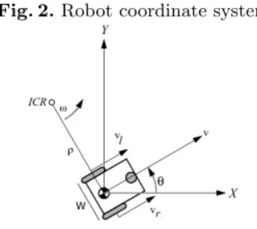
There are two coordinate systems: world coordinate system depicted by XOY
and robot local coordinate system depicted by xoy, the relationship between these two coordinate systems and the relationship of control variables are shown in Fig. 2. The robot is modeled as a differential drive wheeled mobile robot. We
Fig. 2.Robot coordinate system.
can vary the trajectories that the robot takes by varying the velocities υl and υr of the two wheels.
When the mobile robot moves in the unknown environments, the distance to the targetdtand the steering angleθtcan be computed from the robot current
position and target positions in global coordinate.
3
The navigation system
The robot moves in an environment with unknown obstacles. In the following we will ignore all the problems related to position uncertainty (such as wheels drifting), by assuming that a sufficient accurate self-localization subsystem is available. This enables us to use odometry methods to calculate the robot and the target position at every moment. Besides this, the only other source of in-formation available to the robot are the range sensors.
The navigation system consists of three main components:i)target tracking, that finds a set of desired directions from the current robot and target positions; ii)obstacle avoidance, that finds a set of disabled directions from the data avail-able from the range sensors; and iii) get possible direction, that combines the fuzzy conclusions of the previous modules to find a direction that takes into account both the desired and the disabled direction.
3.1 Target tracking
This behavior finds a set of desired directions from the robot actual orientation
θr, which can be obtained at every time interval from the robot actual
posi-tion (xr, yr) and the target position (xT, yT). The rotation angleθg required to
align the robot to the target is calculated from this data. The angle θg is then
translated to a steering set named RIGHT, RIGHT, FRONT, FRONT-LEFT and FRONT-LEFT. The fuzzy rules that perform this translation are:
– IFθg is close to -90, THEN desired-headingis R. – IFθg is close to -45, THEN desired-headingis FR. – IFθg is close to 0, THEN desired-headingis F.
– IFθg is close to 45, THEN desired-headingis FL. – IFθg is close to 90, THEN desired-headingis L.
3.2 Obstacle avoidance
This behavior determines the directionθdin which the robot should be heading
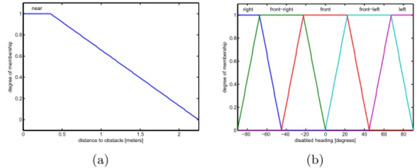
to avoid obstacles. It uses the data available from the range sensors to represent the level in which a given direction (L, FL, F, FR or R) has an obstacle near or not by measuring the degree of membership of each sensed distance to a fuzzy set which we call “near” (see Fig. 3(a)). Each sensor has a steering label (see Fig. 3(b)) that is scaled according to the proximity of obstacles, thus determining the degree of traversability in the vicinity of the robot.
0 0.5 1 1.5 2 0 0.2 0.4 0.6 0.8 1
distance to obstacle [meters]
degree of membership near (a) −80 −60 −40 −20 0 20 40 60 80 0 0.2 0.4 0.6 0.8 1
disabled heading [degrees]
degree of membership
right front−right front front−left left
(b)
Fig. 3. a) Membership function for every sensor. b) Membership functions for the output variableθd.
3.3 Possible direction
This module combines the fuzzy conclusions of thetarget tracking andobstacle avoidance components. We want the robot to be heading towards a direction that takes into account both the desired and the disabled direction. To do this, we realize the following fuzzy operations:
θp=θg AND NOT θd (1)
=θg∩(1−θd) (2)
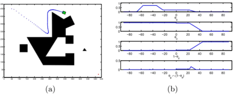
Figures 4(a) shows the robot with obstacles in the right, while Fig. 4(b) shows the output of each of the fuzzy systems, where we can see that θg is trying to
make the robot go to the right, whileθd is disabling this set of directions. The
possible direction module combines these fuzzy sets in a way that makes the robot turn approximately 25◦ to the left.
0 50 100 150 200 250 300 350 400 450 500 550 600640 0 50 100 150 200 250 300 350 400 450 480 (a) −80 −60 −40 −20 0 20 40 60 80 0 0.5 1 θg −80 −60 −40 −20 0 20 40 60 80 0 0.5 1 θd −80 −60 −40 −20 0 20 40 60 80 0 0.5 1 1−θd −80 −60 −40 −20 0 20 40 60 80 0 0.5 θg∩ (1−θd) (b)
Fig. 4.The fuzzy system in action. (a) The robot near obstacles. (b) The output of each of the fuzzy components.
3.4 Deadlock detection and avoidance
Since the robot does not remember the location visited before and the navigation algorithm is based only on local information, it can get trapped in local min-ima commonly called deadlock [11],limit cycle [1, 17] orinfinite loop[6]. While trapped in this situation, the robot will repeat indefinitely the same trajectory unless this is detected and deal with this situation.
Xu et al. [17] detects a deadlock whenever the robot makes a sharp turn while Yang et al. [19] detects a deadlock when all sensors detect small distances to obstacles, both of them produce a set of subgoals that help escape the dead-lock until an escape criterion is met. The algorithm proposed by Xu et al. [17] obtains good results, although in some complicated environments the algorithm may produce a significant quantity of subgoals. It is worth mentioning that Yang et al. [19] experimental results are all with simple maps, where the anti-deadlock mechanism cannot be properly evaluated. Krishna et al. [9] uses a fuzzy classifi-cation scheme coupled to Kohonens self-organizing map and fuzzy ART network determines this classification and Wang et al. [16] builds a memory grid map which records the environmental information and the robot experience while traversing the map. Ordonez et al. [11] uses a virtual wall approach. Our pro-posed method uses the distance to the target dt to detect if the robot is in a
deadlock. At every time interval the navigation algorithm calculates the distance
dt and orientationθt of the robot to the target. If we store the last N records
we could think of the distance as a signal over timedtand see how this behaves
in different situations, being the main case of interest how this signal behaves when the robot is in a deadlock situation.
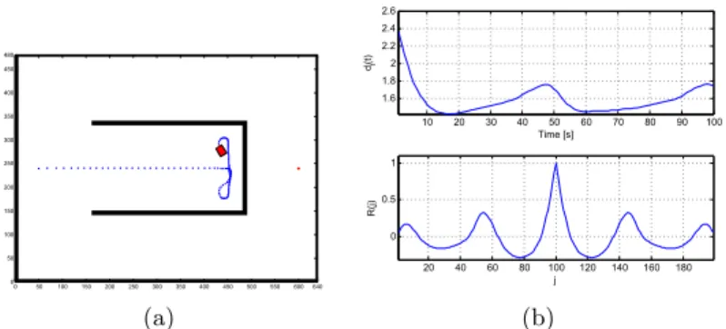
When the robot is in an obstacle free environment , the distance would initially beD0and it would decrease down to 0 . However, when facing a deadlock
situation the robot travels indefinitely along the deadlock loop (see Fig. 5(a)) and the measurements of the distancedtwill then become periodic, as shown in Fig.
5(b). The usual method for deciding if a signal is periodic and then estimating its period is the autocorrelation function. The discrete autocorrelationR at lag
j for a discrete signalxn is defined by R(j) =X
n
xnxn−j. (3)
If the signal is periodic with periodP, the autocorrelationRwill attain a max-imum at sample lags of ±nP, where n ∈Z [13]. We can see in Fig. 5(a), that the size of the traversed path is 148 centimeters and the period of the autocor-relation signal R(j) in Fig. 5(b) is 148. By callingM0=R(0) andM1=R(P),
we can check the periodicity of the signal through
M1 M0
≥τ, (4)
whereτ is a real valued constant defined by the variance of the system noise. If this check gives positive results we can change the robot’s behavior towall-follow and escape the deadlock.
begin
p←−is periodic(d10);
if ¬pthen
p←−is periodic(d20);
end
if ¬deadlock status∧pthen
deadlock status←−T rue;
else
deadlock status←−F alse;
end end
Algorithm 1: Periodicity detection algorithm
3.5 Selecting the window size
The window size plays a critical role in the correct behavior of the deadlock detection algorithm. Small window sizes will detect small sized deadlocks, but will fail to catch the periodicity of big sized deadlocks. On the other side, using a large window will enable us to detect big sized deadlocks, but it will spend much more time until a small sized deadlock fills the window and the deadlock detection method detects the periodicity. Thus, there is a trade-off between the window sizeN, the suspected periodicity size and the time spent to detect the deadlock situation.
We chose to implement a constant size, multi-window approach. The first window is the signaldtand the others being downsampled versions of the first.
We can downsampledtas many times as we want and we can run our detection
algorithm in parallel through all the windows. This enables us to detect deadlocks of various sizes while mantaining a quick response and a small storage space. In
0 50 100 150 200 250 300 350 400 450 500 550 600640 0 50 100 150 200 250 300 350 400 450 480 (a) 10 20 30 40 50 60 70 80 90 100 1.6 1.8 2 2.2 2.4 2.6 dt (t) Time [s] 20 40 60 80 100 120 140 160 180 0 0.5 1 j R(j) (b)
Fig. 5.The robot in a typical deadlock-prone scenario. (a) Simulation results. (b) Evo-lution of the measured distance through time (top) and its autocorrelation (bottom).
our experiments we chose to use two windows of size N = 100, namedd10 and
d20. The second window being the downsampled version of the first, keeping every second sample of the signal and discarding the others. By doing this, we ensure to keep the windows size small enough while catching periodicities of two different sizes that are appropriate for the map sizes we work with. The method used to check if the robot is in a deadlock situation is shown in algorithm 1.
3.6 Wall following
Once the robot knows it is in a deadlock situation it can change its behavior and try to escape from it. We chose to implement a fuzzy logic wall following controller. When the deadlock detection algorithm checks positive, we store the distance to the targetdtas the deadlock distancedland the robot follows a wall
untildt≤dl and|θp|< β, where β is a real valued constant.
3.7 Algorithm
The main navigation algorithm can be seen in algorithm 2.
4
Simulation results
We ran different experiments on various deadlock-prone maps from Wang et al. [16] and compared our algorithm with the “minimum risk method” proposed in this work. The blue lines show the robot traveling in the normal goal-oriented behavior while the red lines show the deadlock-detection and wall-following be-havior.
We first compare our method in concave environments. Figure 6(a) detects a deadlock before making entering the first repetition of the infinite loop. It then follows the left wall until the escape criterion is met and reaches the target.
whiledt≥MIN DISTANCEdo acquire sensor readings;
if deadlock situation then
whiledt≥dldo
compute wall follow direction; wall follow;
end else
compute target directiondp; go to target;
end end
Algorithm 2: Navigation algorithm
Figure 6(b) shows the result of the minimum risk method. The robot exhibits a so-called “trial and return” phenomenon and manages to escape the deadlock. In Wang et al. there are comparison with virtual target methods [18] and Kr-ishna and Kalra’s method [9]. While the first fails to reach the target, the second exhibits a similar behavior as our method by using a fuzzy classification scheme coupled to Kohonen’s self-organizing map (SOM) and fuzzy ART network to determine the deadlock situation. This requires to train the SOM to learn typ-ical landmarks that are expected to occur in a general environment. However, all the experiences of spatio-temporal patterns cannot be modeled through the landmarks learnt offline. Under some situations this can result in the robot not getting aware of its trapped condition and because of this, a Fuzzy ART network is added to dynamically add new patterns to the knowledge base. This archi-tecture is more complicated than our approach, which has only to calculate an autocorrelation.
We next compare our algorithm in a concave environment shown in Fig. 7(a) where we can see that we get similar results that the ones in Fig. 7(b). In Wang et al. it is shown that Krishna and Kalra’s method reaches the target, but choses a wall boundary that leads to a longer traversed path. It is very difficult to choose the correct boundary to follow without making maps or remembering the past as the minimum risk method does.
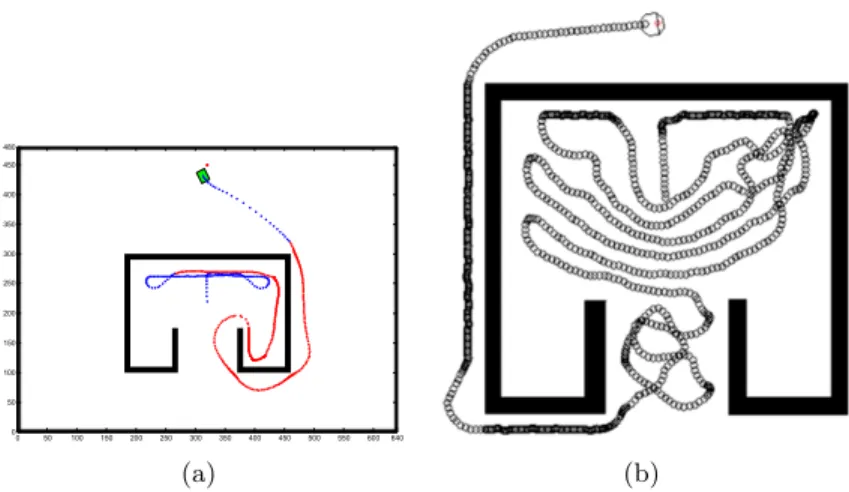
We finally test our algorithm in a complicated environment shown in Fig 4. We can see that the proposed method is capable of reaching the target. It detects and escapes from two different sized deadlocks during the traversal of the environment.
Our method exhibits a behavior similar to Krishna and Kalra’s and the minimum risk method, but is worth to mention that it neither uses a Kohonens self-organizing map nor makes a grid of the traversed path. In this way, the proposed scheme is much simpler while maintaining the effectiveness. The only extra data needed is the distance to the targetdtand a deadlock can be detected
0 50 100 150 200 250 300 350 400 450 500 550 600 640 0 50 100 150 200 250 300 350 400 450 480 (a) (b)
Fig. 6. In large concave and recursive U-shaped environment. (a) Our method. (b) Minimum risk method
0 50 100 150 200 250 300 350 400 450 500 550 600 640 0 50 100 150 200 250 300 350 400 450 480 (a) (b)
Fig. 7.In a concave environment. (a) Our method. (b) Minimum risk method.
0 50 100 150 200 250 300 350 400 450 500 550 600 640 0 50 100 150 200 250 300 350 400 450 480
5
Conclusions
The proposed method is effective and enables the robot to escape from deadlock situations while using as little data as the distance to the target. The obtained results are comparable with methods that use more complex schemes.
It is extremely difficult to guarantee that a selected direction will ensure to leave the deadlock situation once detected. Without further information nothing guarantees that following a wall to the right is better than following it to the left. In unknown environments optimal navigation distance is not known, but travel time can be reduced by controlling the robot’s velocity. The simulation results shown in Section 4 show that the robot reaches every target describing a smooth trajectory. If the method is aimed to be used for long-distance navigation, another information sources should be added, such as a GPS or an IMU unit to compensate the odometry errors.
References
1. Ranajit Chatterjee and Fumitoshi Matsuno. Use of single side reflex for au-tonomous navigation of mobile robots in unknown environments. Robotics and
Autonomous Systems, 35(2):77 – 96, 2001.
2. Wang Dongshu, Zhang Yusheng, and Si Wenjie. Behavior-based hierarchical fuzzy control for mobile robot navigation in dynamic environment. InControl and
De-cision Conference (CCDC), 2011 Chinese, pages 2419–2424. IEEE, 2011.
3. Shuzhi S. Ge and YJ Cui. Dynamic motion planning for mobile robots using potential field method. Autonomous Robots, 13(3):207–222, 2002.
4. Yanrong Hu and Simon X Yang. A knowledge based genetic algorithm for path planning of a mobile robot. In Robotics and Automation, 2004. Proceedings.
ICRA’04. 2004 IEEE International Conference on, volume 5, pages 4350–4355.
IEEE, 2004.
5. G.S. Huang, C.K. Tung, and J.C. Ciou. To achieve the path planning of mobile robot for a correct destination and direction using fuzzy theory. In Industrial
Electronics, 2009. ISIE 2009. IEEE International Symposium on, pages 1737–1742.
IEEE, 2009.
6. K. Madhava Krishna and Prem K Kalra. Solving the local minima problem for a mobile robot by classification of spatio-temporal sensory sequences. Journal of
Robotic Systems, 17(10):549–564, 2000.
7. Qing Li, Xinhai Tong, Sijiang Xie, and Yingchun Zhang. Optimum path plan-ning for mobile robots based on a hybrid genetic algorithm. InHybrid Intelligent
Systems, 2006. HIS ’06. Sixth International Conference on, pages 53–53, 2006.
8. Qing Li, Wei Zhang, Yixin Yin, Zhiliang Wang, and Guangjun Liu. An improved genetic algorithm of optimum path planning for mobile robots. InIntelligent
Sys-tems Design and Applications, 2006. ISDA’06. Sixth International Conference on,
volume 2, pages 637–642. IEEE, 2006.
9. K Madhava Krishna and Prem K Kalra. Perception and remembrance of the envi-ronment during real-time navigation of a mobile robot. Robotics and Autonomous
Systems, 37(1):25–51, 2001.
10. Javier Minguez and Luis Montano. Sensor-based robot motion generation in un-known, dynamic and troublesome scenarios. Robotics and Autonomous Systems, 52(4):290–311, 2005.
11. Camilo Ordonez, Emmanuel G. Collins Jr., Majura F. Selekwa, and Damion D. Dunlap. The virtual wall approach to limit cycle avoidance for unmanned ground vehicles. Robotics and Autonomous Systems, 56(8):645 – 657, 2008.
12. Ruan Qiuqi et al. A gene-constrained genetic algorithm for solving shortest path problem. InSignal Processing, 2004. Proceedings. ICSP’04. 2004 7th International
Conference on, volume 3, pages 2510–2513. IEEE, 2004.
13. Lawrence R Rabiner and Ronald W Schafer. Digital processing of speech signals, volume 19. IET, 1979.
14. A. Saffiotti. The uses of fuzzy logic in autonomous robot navigation. Soft
Computing-A Fusion of Foundations, Methodologies and Applications, 1(4):180–
197, 1997.
15. Jianping Tu and Simon X Yang. Genetic algorithm based path planning for a mobile robot. In Robotics and Automation, 2003. Proceedings. ICRA’03. IEEE
International Conference on, volume 1, pages 1221–1226. IEEE, 2003.
16. Meng Wang and James NK Liu. Fuzzy logic-based real-time robot navigation in unknown environment with dead ends. Robotics and Autonomous Systems, 56(7):625–643, 2008.
17. WL Xu. A virtual target approach for resolving the limit cycle problem in naviga-tion of a fuzzy behaviour-based mobile robot. Robotics and Autonomous Systems, 30(4):315–324, 2000.
18. WL Xu and SK Tso. Sensor-based fuzzy reactive navigation of a mobile robot through local target switching. Systems, Man, and Cybernetics, Part C:
Applica-tions and Reviews, IEEE TransacApplica-tions on, 29(3):451–459, 1999.
19. X. Yang, M. Moallem, and R.V. Patel. A layered goal-oriented fuzzy motion plan-ning strategy for mobile robot navigation. Systems, Man, and Cybernetics, Part
B: Cybernetics, IEEE Transactions on, 35(6):1214–1224, 2005.
20. John Yen and Nathan Pfluger. A fuzzy logic based extension to payton and rosen-blatt’s command fusion method for mobile robot navigation. Systems, Man and
Cybernetics, IEEE Transactions on, 25(6):971–978, 1995.
21. Soh Chin Yun, V. Ganapathy, and Lim Ooi Chong. Improved genetic algorithms based optimum path planning for mobile robot. InControl Automation Robotics