Timing of Convertible Debt Financing and Investment

C A R F W o r k i n g P a p e r

CARF-F-131

Timing of Convertible Debt Financing and

Investment

Katsushige Sawaki Nanzan University

August, 2008

CARF is presently supported by AIG, Bank of Tokyo-Mitsubishi UFJ, Ltd., Citigroup, Dai-ichi Mutual Life Insurance Company, Meiji Yasuda Life Insurance Company, Mizuho Financial Group, Inc., Nippon Life Insurance Company, Nomura Holdings, Inc. and Sumitomo Mitsui Banking Corporation (in alphabetical order). This financial support enables us to issue CARF Working Papers.

CARF Working Papers can be downloaded without charge from: http://www.carf.e.u-tokyo.ac.jp/workingpaper/index.cgi

Working Papers are a series of manuscripts in their draft form. They are not intended for circulation or distribution except as indicated by the author. For that reason Working Papers may not be reproduced or distributed without the written consent of the author.

Timing of Convertible Debt Financing and

Investment

Kyoko Yagi

_{Ryuta Takashima}

Hiroshi Takamori

_{Katsushige Sawaki}

1_{Center for Advanced Research in Finance, The University of Tokyo}

7-3-1 Hongo, Bunkyo-ku, Tokyo 113-0033, Japan, E-mail: yagi@e.u-tokyo.ac.jp

2_{Department of Nuclear Engineering and Management, The University of Tokyo}

7-3-1 Hongo, Bunkyo-ku, Tokyo 113-8656, Japan, E-mail: takashima@n.t.u-tokyo.ac.jp

3_{Graduate School of Policy Studies, Chiba University of Commerce}

1-3-1 Kokufudai, Ichikawa-shi, Chiba 272-8512, Japan, E-mail: takamori.hiro@gmail.com

4_{Graduate School of Business Administration, Nanzan University}

18 Yamazato-cho, Showa-ku, Nagoya, Aichi 466-8673, Japan, E-mail: sawaki@nanzan-u.ac.jp

Abstract

In this paper, we examine the optimal investment policy of the firm which is financed by issuing equity, straight debt and convertible debt. We extend the model in Mauer and Sarkar [7] over financing with convertible debt. We examine two different investment policies that maximize the equity value and the firm value and show the agency cost as the difference between each policy value. Furthermore, we investigate how the issuance of convertible debt affects investment.

Keywords: Real options, convertible debt, investment, agency cost

1

Introduction

Real options theory, pioneered by Brennan and Schwartz [2], and McDonald and Siegel [9], and summarized in Dixit and Pindyck [3], has attracted growing attention because it enables us to account for the value of flexibility under uncertainty. In standard real options models, all-equity financing is assumed, and the interactions between investment and financing decisions have been not analyzed.

Recently many researchers have studied the interaction among firm’s investment and financ-ing decisions under uncertainty by means of real option framework. In some literatures, the investment problems for the firm with growth options, which is financed with equity and debt are investigated (e.g. Lyandres and Zhdanov [4], Mauer and Ott [6], Mauer and Sarkar [7], and

Sundaresan and Wang [10]). Although the debt used in these studies is straight debt, there also exists a previous work on the effect of convertible debt financing on the investment decisions. Lyandres and Zhdanov [5] suggests the model for analyzing the investment problem of the firm with outstanding convertible debt and discusses the accelerated investment effect arising from the issuance of convertible debt by the optimal investment policy to maximize the equity value. In their model, the value of the firm, which is the sum of the equity and debt values, and the leverage ratio are not analyzed.

In this paper, we examine the optimal investment policy of the firm which is financed by issuing equity, straight debt and convertible debt. We extend the model in Mauer and Sarkar [7] over financing with convertible debt in the following section. As in Mauer and Sarkar [7], we examines two different investment policies that maximize the equity value and the firm value. In Sec. 3 we discuss a difference of the optimal investment policies maximizing between the value of equity and the firm value by issuing convertible debt, and then show the agency cost as the difference between each policy value by using numerical results. Furthermore, we investigate how the issuance of convertible debt affects investment. Finally, in Sec. 4 we summarize this paper with some concluding remarks.

2

The Model

Consider a firm with an option to invest at any time by paying a fixed investment costI. The firm partially finances the cost of investment with straight debt and convertible debt. Denote

Ks as the total issue value of straight debt with the instantaneous contractual coupon payment

of s and infinite maturity, and Kc as that of convertible debt with coupon payment of c and

infinite maturity. These coupon payments are tax-deductible at a constant corporate tax rateτ. Once the investment option is exercised, we assume that the firm can receive the instantaneous profit

π(xt) = (1−τ)(xt−s−c), (1)

where xt is the firm’s instantaneous EBIT. Suppose that xt is given by a geometric Brownian

motion

dxt=µxtdt+σxtdWt, (2)

whereµ and σ are the risk-adjusted expected growth rate and the volatility of xt, respectively,

and Wt is a standard Brownian motion defined on a probability space (Ω, F,P). We assume

that the holders of convertible debt can convert the debt into a fractionηof the original equity, whereη=αcandα is a constant. In this paper we deal with only non-callable convertible debt. In order to examine two different investment policies which maximize the equity value and the firm value and investigate how the issue of convertible debt influences investment, we consider several settings. First, we present a benchmark model in which the investment is financed with

all-equity. Second, we examine the case in that the investment is financed with equity and straight debt, based on the analysis in Mauer and Sarkar [7]. Third, we model the investment financed with equity and convertible debt. Finally, we consider the firm with an option of investment that is financed with equity and both debt.

2.1 All-Equity Financing

In this section we assume that the investment is financed entirely with equity (s= 0 andc= 0). This case has been studied in the literature on real options (e.g. Dixit and Pindyck [3] and McDonald and Siegel [9]).

The optimal investment rule is to exercise the investment option at the first passage time of the stochastic shock to an upper threshold x∗. Assuming that the pre-investment profit of the firm is zero, the value of an investment option F(x0) can be formulated as

F(x0) = sup T∗>0 Ex0 [ e−rT∗ {∫ _∞ T∗ e−r(u−T∗)(1−τ)xudu−I } ] , (3)

whereT∗ is a stopping time (investment time) whenxtreaches the investment thresholdx∗,Ex0

is the conditional expectation operator given that the EBIT at time 0 is equal to x0, and r is

the risk-free interest rate. For convergence, we assume r > µ.

Since the ordinary differential equation, which is satisfied by the value of investment option in Eq. (3), is derived from Bellman equation1:

1 2σ 2_x2d2F dx2 +µx dF dx −rF = 0 (4)

forx < x∗, the general solution of Eq. (4) is given by

F(x) =a1xβ1 +a2xβ2, x < x∗, (5) where β1 = 1₂ − _σµ2 + √(₁ 2 − µ σ2 )2 +_σ2r2 > 1 and β2 = 1₂ − _σµ2 − √(₁ 2− µ σ2 )2 +2_σr2 < 0. Using

standard arguments, a2 = 0 and the investment threshold x∗ is given by

x∗ = β1

β1−1

r−µ

1−τI. (6)

Then, the value of the investment optionF(x0) is given by

F(x0) = (_x 0 x∗ )β1 (²(x∗)−I), x0 < x∗, (7)

where ²(x) is the total post-investment profit in which the investment is financed entirely with equity,

²(x) = (1−τ)x

r−µ . (8)

From β1 >1 and r > µ, the investment threshold x∗ > I. This means that the investment is

made when the EBIT is higher than the investment cost.

1

2.2 Equity and Straight Debt Financing

Next we consider a firm which has an option of the investment that is financed with equity and straight debt (s >0 and c= 0), introduced in Mauer and Sarkar [7], and Sundaresan and Wang [10].

2.2.1 Optimal Policies after Investment

In this section we model the values of equity and straight debt after the exercise of investment option. Once the investment option has been exercised, the optimal default policy is established from the issue of debt. The optimal default strategy of the equity holders maximizes the equity value, selecting the default threshold xd. Letting the earnings xt at investment timet equalx,

the optimization problem of the equity holders can be given by

E(x) = sup Td>0 Ex [ ∫ Td t e−r(u−t)(1−τ)(xu−s)du ] , (9)

whereTd is the stopping time on reaching the default threshold xd. Using standard arguments

as in Sec. 2.1, the equity value E(x) is given by

E(x) =²(x)−(1−τ)s r − ( x xd )β2( ²(xd)− (1−τ)s r ) (10) forx > xdand the default thresholdxdis

xd=

β2

β2−1

s(r−µ)

r . (11)

Let Ds(x) be the total value of straight debt issued at investment timet. Since the holders

of straight debt can receive the continuous coupon payment of s, the value of straight debt is given by Ds(x) =Ex [ ∫ Td t e−r(u−t)sdu+e−r(Td−t)₍₁−_θ)²(x Td) ] , (12)

whereθis the proportional bankruptcy cost, 0≤θ≤1. The holders of straight debt are entitled to the unlevered value of the firm net of proportional bankruptcy cost, (1−θ)²(x) at bankruptcy. Then, the value of straight debt is given by

Ds(x) = s r − ( x xd )β2(_s r −(1−θ)²(xd) ) , x > xd. (13)

The sum of E(x) in Eq. (10) andDs(x) in Eq. (13) gives the firm value as

Vs(x) =E(x) +Ds(x) =²(x) + τ s r { 1− ( x xd )β2} −θ²(xd). (14)

The firm value Vs(x) is decomposed into the value of unlevered firm ²(x), the expected present

2.2.2 Optimal Investment Policy

Here we consider the optimal investment policy. First, we examine the optimal policy maximizing the value of equity, not total firm value. Denotex∗₂ as the second-best investment threshold. By the optimal policy selecting x∗₂ to maximize the equity value (9), the value of the investment option F2(x0) is given by F2(x0) = sup T2∗>0 Ex0 [ e−rT2∗{_E(x T₂∗)−(I−Ks) }] , (15)

whereT₂∗is the stopping time on reaching the investment thresholdx∗₂, andKsis the total values

of straight debt issued at investment. Using the value matching and smooth-pasting conditions at the investment threshold, the value of the investment option is given by

F2(x0) = ( x0 x∗₂ )β1 {E(x∗₂)−(I−Ks)} (16)

forx0 < x∗2 and the investment threshold x∗2 is given by the numerical solution of

E(x∗₂)−x ∗ 2 β1 dE dx(x ∗ 2)−(I−Ks) = 0, (17)

whereKs is given by the value of straight debt at the investment threshold x∗2,

Ks =Ds(x∗2) = s r − ( x∗₂ xd )β2(_s r −(1−θ)²(xd) ) . (18)

Noticing thatKs=Ds(x∗2) in Eq. (18) andVs(x∗2) =E(x∗2) +Ds(x∗2), Eq. (16) can be rewritten

as F2(x0) = ( x0 x∗₂ )β1 {Vs(x∗2)−I}. (19)

Next, we analyze the optimal investment policy maximizing the firm value. By choosing the first-best investment thresholdx∗₁ and maximizing the firm valueVs(x) in Eq. (14), the value of

the investment optionF1(x0) is given by

F1(x0) = sup T₁∗>0E x0 [ e−rT1∗{_Vs(x T1∗)−I }] , (20)

where T₁∗ is the stopping time on reaching the threshold x∗₁. For x0 < x∗1 the value of the

investment option is F1(x0) = ( x0 x∗₁ )β1 {Vs(x∗1)−I} (21)

and the investment threshold x∗₁ is numerically solvable from

Vs(x∗1)− x∗₁ β1 dVs dx(x ∗ 1)−I = 0. (22)

2.3 Equity and Convertible Debt Financing

In this section we consider a firm which has an option of the investment that is financed with equity and convertible debt (s= 0 andc >0). In this case the optimal problems of the equity holders and the convertible debt holders have to be solved simultaneously. The optimal policy of the equity holders maximizes the equity value selecting the default threshold. On the other hand, the optimal policy of the convertible debt holders maximizes the value of convertible debt selecting the conversion threshold. We follow Brennan and Schwartz [1] and assume block conversion. This means that all convertible debt holders exercise the conversion option at the same time.

2.3.1 Optimal Policies after Investment

We examine the values of equity and convertible debt issued at investment time. The equity holders optimally select the default thresholdxd, maximizing the equity value. The equity value

at investment time is given by

E(x) = sup Td>0 Ex [ ∫ Tc∧Td t e−r(u−t)(1−τ)(xu−c)du+ 1_{Tc<Td} 1 1 +η ∫ _∞ Tc e−r(u−t)(1−τ)xudu ] , (23) where Td is the stopping time on reaching the default threshold xd, Tc is the stopping time on

reaching the conversion thresholdxc selected by the convertible debt holders, and 1_{Tc<Td} is an

indicator function that is equal to one if Tc < Tdand is equal to zero otherwise. By converting

the equity value is diluted, that is, ₁₊1_η is the dilution factor.

Let Dc(x) be the total value of convertible debt issued at investment time t. The holders of

convertible debt receive the continuous coupon payment ofcand choose the optimal conversion thresholdxc, maximizing the value of convertible debt. Then, the total value of convertible debt

issued at investment time is given by

Dc(x) = sup Tc>0 Ex [ ∫ Tc∧Td t e−r(u−t)cdu+ 1_{Td<Tc}e−r(Td−t)₍₁−_θ)²(x Td) +1_{Tc<Td} η 1 +η ∫ _∞ Tc e−r(u−t)(1−τ)xudu ] . (24)

The holders of convertible debt are entitled to (1−θ)²(x) at bankruptcy.

Once the convertible debt has been converted, the firm becomes an all-equity entity. It follows from the optimal problems of the equity holders and convertible debt holders in (23) and (24), respectively, that the values of equity and convertible debt prior to default and conversion are given by E(x) =a3xβ1 +a4xβ2+ (1−τ) ( x r−µ− c r ) , (25) Dc(x) =a5xβ1 +a6xβ2+ c r. (26)

Constants ai, i = 3,· · · ,6, the default threshold xd and the conversion threshold xc must be

determined using the following boundary conditions:

a3xβd1 +a4xβd2+ (1−τ) ( xd r−µ− c r ) = 0, (27) β1a3xβd1−1+β2a4xβd2−1+ 1−τ r−µ = 0, (28) a3xβc1 +a4xβc2+ (1−τ) ( xc r−µ− c r ) = 1 1 +η (1−τ)xc r−µ , (29) a5xβd1 +a6xβd2+ c r = (1−θ) (1−τ)xd r−µ , (30) a5xβc1 +a6xβc2+ c r = η 1 +η (1−τ)xc r−µ , (31) β1a5xβc1−1+β2a6xβc2−1= η 1 +η 1−τ r−µ. (32)

Eqs. (27), (28) and (30) represent conditions in default. Eq. (27) is the value matching condition which ensures that the value of equity at the default threshold is equal to zero. Eq. (28) is the smooth-pasting condition that ensures the optimality of the the default threshold xd. Eq. (30)

is the value-matching condition which ensures that the value of convertible debt at default threshold equals the unlevered value of the firm net of proportional bankruptcy cost. Eqs. (29), (31) and (32) represent conditions in conversion. Eq. (29) is the value matching condition requiring that the value of equity at the conversion threshold is equal to a proportion of the unlevered value of the firm possessed by the original equity holders after conversion. Eq. (31) is the value matching condition which ensures that the value of convertible debt at the conversion threshold is equal to the value of new equity issued in conversion. Eq. (32) is the smooth-pasting condition that ensures the optimality of the the conversion thresholdxc. Six equations (27)–(32)

have six unknown variables (ai, i= 3,· · · ,6, xd, xc). We can solve these equations numerically.

Then, the firm value Vc(x) is given by

Vc(x) =E(x) +Dc(x) =²(x) +

τ c

r + (a3+a5)x

β1 _{+ (a}

4+a6)xβ2. (33)

2.3.2 Optimal Investment Policy

We examine two optimal investment policies to maximize the equity value (23) and the firm value (33). From Sec. 2.2.2 both the values of the investment option are given by

Fi(x0) = ( x0 x∗_i )β1 {Vc(x∗i)−I} (34)

for x0 < x∗i and i = 1,2. The second-best investment threshold x∗2 is given by the numerical

solution of E(x∗₂)− x ∗ 2 β1 dE dx(x ∗ 2)−(I −Dc(x∗2)) = 0, (35)

and the first-best investment threshold x∗₁ is given by the solution of

Vc(x∗1)− x∗₁ β1 dVc dx(x ∗ 1)−I = 0. (36)

2.4 Equity, Straight Debt and Convertible Debt Financing

In this section we consider a firm with an option of the investment that is financed with eq-uity, straight debt and convertible debt (s > 0 and c > 0). For simplicity reasons, we as-sume that straight debt and convertible debt have the same priority. Hence, the holders of straight debt are entitled to _s+s_c(1−θ)²(x) at pre-conversion bankruptcy and (1−θ)²(x) at post-conversion bankruptcy. Similarly, the convertible debt holders are entitled to _s+c_c(1−θ)²(x) at pre-conversion bankruptcy.

2.4.1 Optimal Policies after Investment

We now model the values of equity, straight debt and convertible debt after the investment option has been exercised. The equity holders optimally select two default thresholds; the pre-conversion default threshold xd and the post-conversion default threshold xd,c, maximizing

the equity value. The optimal post-conversion default threshold xd,c is not equal to the

pre-conversion default onexd, because debt decreases when convertible debt is converted into equity.

The total value of equity at investment time is given by

E(x) = sup Td,Td,c>0 Ex [ ∫ Tc∧Td t e−r(u−t)(1−τ)(xu−s−c)du +1_{Tc<Td} 1 1 +η ∫ Td,c Tc e−r(u−t)(1−τ)(xu−s)du ] , (37)

where Td and Td,c are the stopping times when xt reach the default thresholds xd and xd,c,

respectively, andTc is the stopping time on reaching the conversion thresholdxc.

The value of the straight debt issued at investment time is given by

Ds(x) =Ex [ ∫ Tc∧Td t e−r(u−t)sdu+ 1_{Td<Tc}e−r(Td−t) s s+c(1−θ)²(xTd) +1_{Tc<Td} ( ∫ Td,c Tc e−r(u−t)sdu+e−r(Td,c−t)₍₁−_θ)²(x Td,c) )] . (38)

Similarly, the value of convertible debt at investment time is given by

Dc(x) = sup Tc>0 Ex [ ∫ Tc∧Td t e−r(u−t)cdu+ 1_{Td<Tc}e −r(Td−t) c s+c(1−θ)²(xTd) +1_{Tc<Td} η 1 +η ∫ Td,c Tc e−r(u−t)(1−τ)(xu−s)du ] . (39)

Once the convertible debt has been converted, the firm becomes an entity that issues equity and straight debt and the optimal default policy is established as in Sec. 2.2.1. Let Ea(x) and

Ds,a(x) be the post-conversion total values of equity and straight debt. Lettingxt at conversion

of straight debt Ds,a(x) are given by xd,c= β2 β2−1 s(r−µ) r , (40) Ea(x) =²(x)− (1−τ)s r − ( x xd,c )β2( ²(xd,c)− (1−τ)s r ) , (41) Ds,a(x) = s r − ( x xd,c )β2(_s r −(1−θ)²(xd,c) ) . (42)

Next, we consider the values prior to conversion. It follows from the optimal problems of the equity holders, straight debt holders and convertible debt holders in (37), (38) and (39), respectively, that the values of equity, straight debt and convertible debt prior to default and conversion are given by

E(x) =a7xβ1 +a8xβ2 + (1−τ) ( x r−µ− s+c r ) , (43) Ds(x) =a9xβ1 +a10xβ2+ s r, (44) Dc(x) =a11xβ1 +a12xβ2 + c r. (45)

Constantsai,i= 7,· · · ,12, the pre-conversion default thresholdxdand the conversion threshold

xc are determined by the boundary conditions:

a7xβ_d1+a8xβ_d2 + (1−τ) ( xd r−µ− s+c r ) = 0, (46) β1a7xβ_d1−1+β2a8xβ_d2−1+ 1−τ r−µ = 0, (47) a7xβc1+a8xβc2 + (1−τ) ( xc r−µ− s+c r ) = 1 1 +ηEa(xc), (48) a9xβ_d1 +a10xβ_d2+ s r = s s+c(1−θ) (1−τ)xd r−µ , (49) a9xβc1 +a10xβc2+ s r =Ds,a(xc), (50) a11xβ_d1 +a12xβ_d2+ c r = c s+c(1−θ) (1−τ)xd r−µ , (51) a11xβc1 +a12xβc2+ c r = η 1 +ηEa(xc), (52) β1a11xβc1−1+β2a12xβc2−1 = η 1 +η dEa dx (xc), (53)

where Ea(x) and Ds,a(x) are given in Eqs. (41) and (42). Eqs. (46), (47), (49) and (51) are

conditions in default. On the other hand, Eqs. (48), (50), (52) and (53) are conditions in conversion. Eq. (46) is the value matching condition which ensures that the equity value at the default threshold equals zero. Eq. (47) is the smooth-pasting condition that ensures the optimality of the default threshold xd. Eqs. (49) and (51) are the value matching conditions

which ensure that the values of debt are equal to respective fractions of the unlevered value of the firm net of proportional bankruptcy cost. Eq. (48) is the value matching condition requiring that the value of equity at the conversion threshold equals a proportion of the post-conversion

value of equity given in Eq. (41). Eq. (50) is the value matching condition which ensures that the pre-conversion value of straight debt equals the post-conversion value of straight debt. Equation (52) is the value matching condition which ensures that the value of the convertible debt at the conversion threshold is equal to a proportion of the post-conversion value of equity. Eq. (53) is the smooth-pasting condition that ensures the optimality of the conversion threshold

xc. Eight equations (46)-(53) have eight unknown variables (ai, i = 7,· · ·,12, xd, xc). These

equations can be solved numerically.

Then, the firm value Vs+c(x) is given by

Vs+c(x) =E(x)+Ds(x)+Dc(x) =²(x)+

τ(s+c)

r +(a7+a9+a11)x

β1_+(a

8+a10+a12)xβ2. (54)

2.4.2 Optimal Investment Policy

By the optimal investment policies to maximize the value of equity and the firm value, both the values of the investment option are

Fi(x0) = ( x0 x∗_i )β1 {Vs+c(x∗i)−I} (55)

forx0 < x∗i and i= 1,2. The second-best investment thresholdx∗2 is numerically solvable from

E(x∗₂)−x ∗ 2 β1 dE dx(x ∗ 2)−(I−Ds(x2∗)−Dc(x∗2)) = 0, (56)

and the first-best investment threshold x∗₁ is given by the solution of

Vs+c(x∗1)− x∗₁ β1 dVs+c dx (x ∗ 1)−I = 0. (57)

3

Numerical Analysis

3.1 Investment Option and Agency Cost

In this section, the calculation results of the value of equity, each debt, and the investment option are presented in order to quantify the agency cost. We use the following base case parameters:

µ= 0.01, σ= 0.2, r= 0.05, I= 5, s= 0.15, c= 0.15, α= 1.5, θ= 0.3, τ = 0.3.

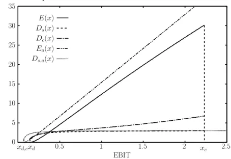
Fig. 1 shows the values of equity, straight debt and convertible debt as functions of the earningx at issue time and the post-conversion values of equity and straight debt as functions of the earningxat conversion time in the case of Sec. 2.4, that is, the investment is financed with equity, straight debt and convertible debt. As can be seen in this figure, the threshold values for the pre-conversion default, the post-conversion default and the conversion are 0.140, 0.069 and 2.229, respectively. These values can provide the investment value of the firm financed by issuing equity, straight debt and convertible debt.

In Fig. 2, the investment values and the threshold values of the investment for the firm-value-maximizing and the equity-firm-value-maximizing policies are shown. It turns out that the

threshold value of the equity-value-maximizing policy is smaller than that of the firm-value-maximizing policy. Thus, like the model in Mauer and Sarkar [7], the equity-value-firm-value-maximizing policy overinvests compared to the firm-value-maximizing policy. Furthermore, at the current value x0 of 0.3, the investment option values for the firm-value-maximizing and

equity-value-maximizing policies are 1.959 and 1.882, respectively. The difference between these values for each policy, that is, the agency cost of overinvestment is 0.077. A proportion of the agency cost to the equity-value-maximizing policy, which is the loss in firm value, is 4.1%. It seems that the agency cost in this case is relatively large compared with that in the case of the firm which has only straight debt as in Mauer and Sarkar [7]. In this section, we consider the case that the investment is financed with equity, straight debt and convertible debt. In order to compare the property of convertible debt with that of straight debt, we explore the investment financed with equity and convertible debt (but no straight debt), and equity and straight debt (but no convertible debt) in the next section.

3.2 Comparison of Convertible Debt and Straight Debt

Here we analyze the investment decision in which the firm issues convertible debt. In this section, the following set of parameters is used: x0 = 0.3, µ = 0.01, σ = 0.2, r = 0.05, I = 5, α =

1.5, θ= 0.3, τ = 0.3.

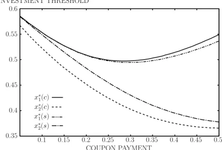
Fig. 3 shows the first-best and second-best investment thresholds as functions of coupon payment, c or s, in the case that the firm is financed with equity and either straight debt or convertible debt in Sec.2.2 and 2.3. For the first-best investment policy, convertible debt leads to underinvestment relative to straight debt. Once the investment is financed with debt, the firm can enjoy interest tax shields, and so can have a tax incentive to accelerate the investment. Since convertible debt includes the option to convert debt into equity, the presence of the op-tion reduces the magnitude of the tax shield effect. This leads to an incentive to speed down investment. On the other hand, for the second-best investment policy, convertible debt leads to overinvestment relative to straight debt. The equity holders are not affected by the benefit of the debt holders, and are therefore indifferent to increased risk of default resulting from the earlier investment. As can be seen in Fig. 4, since the convertible debt includes the conversion option, the default probability of convertible debt is higher than that of straight debt. This means that the equity holders optimally hope to exercise the option prior to the convertible debt holders. Similarly, the convertible debt holders also wish to exercise the option, optimally, prior to the equity holders. Hence, by investing earlier, the equity holders can shift the default risk to the debt holders, can raise the probability of conversion for the convertible debt holders, and can mitigate the disposition of the welfare to debt holders.

0 5 10 15 20 25 30 35 0.5 1 1.5 2 2.5

VALUE OF EQUITY AND DEBT

EBIT Ds,a(x) Ea(x) Dc(x) Ds(x) E(x) xd,cxd xc

Figure 1: Equity, straight debt and convertible debt

µ= 0.01, σ= 0.2, r = 0.05, s= 0.15, c= 0.15, α= 1.5, θ= 0.3, τ = 0.3 -4 -3 -2 -1 0 1 2 3 4 5 6 0 0.1 0.2 0.3 0.6 OPTION VALUE EBIT Vs+c(x0)−I F2(x0) F1(x0) x∗ 2 x∗1 xd

Figure 2: Investment option

0.35 0.4 0.45 0.5 0.55 0.6 0.1 0.15 0.2 0.25 0.3 0.35 0.4 0.45 0.5 COUPON PAYMENT x∗ 2(s) x∗ 1(s) x∗ 2(c) x∗ 1(c) INVESTMENT THRESHOLD

Figure 3: Investment threshold

µ= 0.01, σ = 0.2, r= 0.05, I = 5, α= 1.5, θ= 0.3, τ = 0.3 0 0.05 0.1 0.15 0.2 0.25 0.05 0.1 0.15 0.2 0.25 0.3 0.35 0.4 0.45 0.5 DEFAULT THRESHOLD COUPON PAYMENT xd(s) xd(c)

Figure 4: Default threshold

4

Summary

In this paper, we have investigated the optimal investment policy of the firm financed by issuing equity, straight debt and convertible debt. The values of equity, straight debt and convertible debt after exercising the investment option were shown. We also showed the investment option value and the threshold value for the firm-value-maximizing and equity-value-maximizing poli-cies. In particular, we found that the issue of convertble debt for the firm-value-maximizing policy leads to underinvestment relative to that of straight debt. On the other hand, the issue of convertble debt for the equity-value-maximizing policy leads to overinvestmeCCCCnt relative to that of straight debt.

Many convertible debt contracts include call provisions which entitle the firm to repurchase its debt. For future works, therefore, we will examine the effect of callable convertible debt on investment decision as in Lyandres and Zhdanov [5]. In addition, as discussed in Mayers [8], con-vertible debt provides a firm with sequential investments with an advantage. Possible extension of this study also includes an analysis of multi-stage investment project.

References

[1] Brennan, M.J. and E.S. Schwartz, Convertible Bonds: Valuation and Optimal Strategies for Call and Conversion, Journal of Finance,32, pp.1699-1715, (1977).

[2] Brennan, M.J. and E.S. Schwartz, Evaluating Natural Resource Investment,Journal of Busi-ness,58, pp.135-157, (1985).

[3] Dixit, A. and R. Pindyck,Investment under Uncertainty, Princeton University Press, Prince-ton, 1994.

[4] Lyandres, E. and A. Zhdanov, Accelerated Financing and Investment in the Presence of Risky Debt,Simon School Working Paper, No. FR 03-28, (2006).

[5] Lyandres, E. and A. Zhdanov, Convertible Debt and Investment Timing,working paper, Rice University, (2006).

[6] Mauer, D.C. and S. Ott, Agency Costs, Underinvestment, and Optimal Capital Structure: The Effect of Growth Options to Expand, in M. Brennan and L. Trigeorgis(eds.), Project Flexibility, Agency, and Competition: New Developments in the Theory and Application of Real Options, Oxford University Press, New York, pp.151-180, 2000.

[7] Mauer, D.C. and S. Sarkar, Real Option, Agency Conflicts, and Optimal Capital Structure,

[8] Mayers, D., Why Firms Issue Convertible Bonds: The Matching of Financial and Real Investment Options, Journal of Financial Economics,47, pp.83-102, (1998).

[9] McDonald, R. and D. Siegel, The Value of Waiting to Invest,Quarterly Journal of Economics, 101, pp.707-727, (1986).

[10] Sundaresan, S. and N. Wang, Dynamic Investment, Capital Structure, and Debt Overhang,