Expanding Agricultural Production in Tanzania

(1)

Working paper

Expanding

Agricultural

Production

in Tanzania

Scoping Study for

IGC Tanzania on

the National Panel

Surveys

Vincent Leyaro

Oliver Morrissey

April 2013

(2)

EXPANDING AGRICULTURAL PRODUCTION IN

TANZANIA

Scoping Study for IGC Tanzania on the National Panel Surveys

Dr Vincent Leyaro, University of Dar-es-Salaam Professor Oliver Morrissey, University of Nottingham

April, 2013

CONTENTS Purpose and Aims

1. Context: Agriculture in Tanzania

2. Overview of Agricultural Policy and Performance 3. Data Measures and Definitions

4. Descriptive Statistics from NPS 2007/08 and 2010/11 5. Phase II Proposal: Productivity and Supply Response References

(3)

Purpose and Aims

As agriculture accounts for a large share of employment, export earnings and even GDP in Tanzania, the sector is seen as a main vehicle in any national economic strategy to combat poverty and enhanced agricultural productivity is crucial to realize this objective. Despite this, there are no comprehensive studies of agricultural production and productivity using farm-level data in Tanzania. The National Panel Surveys (NPS) of 2008/09 and 2010/11 provide extensive data on some 3,280 farm households sampled throughout Tanzania, including information on area planted, quantity and value of harvest and input use (purchased and household) for a wide a variety of crops. Analysis of these panels offers the potential to provide insight on the determinants of productivity and supply response, in particular to identify factors amenable to policy influence that can provide effective incentives for farmers to increase production and efficiency. The basic aim of the scoping study is to assess the potential of analysing this data by describing and summarising the information.

Principal aims:

1. Detail and describe the available farm-level data on production, value and input use classified by principal crops and regions.

2. Establish the current status of output, yield and return (value of output) per acre by crop and regions.

3. Identify crops with growth potential in terms of output and productivity.

4. Show that appropriate data are available to estimate supply response and determinants of yield and production.

(4)

1 Context: Agriculture in Tanzania

After 50 years of independence, despite apparent commitment to policies and strategies to transform the agriculture sector, performance in agricultural output and productivity has been disappointing. Policies and plans, such as ‘agriculture is the mainstay of the economy’ and Kilimo Kwanza (agriculture first), have remained slogans to the public as there is so little experience of reforms that have improved livelihoods and millions in the agriculture sector remain in poverty. Tanzania is endowed with considerable fertile agricultural land and inland fresh water resources that can be utilized for irrigation, but much of the land is underutilized and what is utilised often exhibits very low productivity. In this sense Tanzania has yet to achieve the traditional ‘structural transformation’ whereby increasing agricultural production provides a platform for manufacturing and economic growth. Balanced growth is achieved if agriculture becomes increasingly commercialized while the manufacturing sector grows. Initially manufacturing may be based on agriculture, through processing and agri-business, but ultimately manufacturing and the economy will become diversified. This has not happened in Tanzania, and the economy remains essentially agriculture-based, mostly a peasant economy with low productivity. Understanding the factors that can expand production and enhance agricultural productivity in Tanzania is critical for ensuring ‘structural transformation’ and economic growth, boosting development and reducing poverty (given that the majority of the poor are in rural areas).

Some 80 per cent of Tanzanians depend on agriculture for their livelihood; the sector accounts for about 50 per cent of GDP and 75 per cent of export earnings. Consequently, the National Development Vision 2025, the main national development strategy in Tanzania, places considerable emphasis on the sector and envisages that by 2025 the economy will have been transformed from a low productivity agricultural economy to a semi-industrialized one led by modernized and highly productive agricultural activities that are integrated with industrial and service activities in urban and rural areas. Against this background, in the last decade a number of polices and strategies have been formulated to support agriculture in a more systematic way. The Agricultural Sector Development Strategy (ASDS) was adopted in 2001, and gave rise to the Agricultural Sector Development Program (ASDP) of 2005; and the Cooperative Development Policy (CDP) of 2002, complemented by a variety of sector policies. The strategy and the ASDP are embedded in the National Strategy for Growth and Reduction of Poverty (NSGRP), which is a medium term plan to realize Vision 2025. Kilimo 3

(5)

Kwanza (agriculture first), developed in 2009, provides additional inputs for the implementation of ASDP and other programs favourable for the agricultural sector. It is an assertion of the commitment of the government and the private sector to agricultural development, and it invites all Tanzanians to become part of this commitment. Its ten pillars support the ASDS and the ASDP and strengthen them by adding additional initiatives, in particular in rural finance.

The agriculture sector is therefore seen as a main vehicle in any national economic strategy to combat poverty, enhanced agricultural productivity is crucial to realize the objectives, and the policy statements have at least identified the issues and proposed a strategy. The ASDS emphasized the need to improve the efficiency of input markets and product marketing, increase access to credit, enhance the provision of extension services and increase investment in rural areas (especially for irrigation and transport). The ASDP was in principle the strategy to implement these aims, but had limited impact – the strategies were not a success. Thus, the culmination of these initiatives was the formulation of a belief in the need to ‘reintroduce selective subsidies, particularly for agricultural inputs, machinery and livestock development inputs and services’ (ESRF, 2005: xii). The second phase of the research, by providing some quantitative assessment of the importance of different factors (such as prices, access to credit and other inputs, access to markets and marketing) to output levels for the major crops, will contribute to understanding why the strategy has failed and providing recommendations of factors to target for an effective strategy.

Despite the CDP, the cooperative sector has failed to respond to the challenge of liberalization. The sector suffers from weak managerial (and advocacy) skills, a lack of financial resources (in particular undercapitalization of cooperative banks, so credit constraints remain), and a weak institutional structure (especially in that they are not accountable to members). Thus, although the cooperative sector remains significant it is not viewed as successful, either in supporting development and growth or in representing the interests of members, giving added impetus to liberalization initiatives.

Agriculture is recognized as integral to the Poverty Reduction Strategy, and agricultural sector growth is essential if Tanzania is to achieve sustained economic development. While this may seem somewhat obvious, it marks a change in emphasis – the whole sector (not only export crops) has attained a higher status on the policy (and political) agenda, and a view is emerging that there is a need for positive support to the sector. In this context, it is timely to attempt to assess the determinants of production and productivity in 4

(6)

agriculture using crop and farm level data. This scoping study aims to assess the types of productivity and supply response analysis that can be undertaken with the NPS data.

2 Overview of Agricultural Performance

There was some growth in agriculture, especially food production, in the latter half of the 1980s that contributed to increasing the income and welfare of rural households, and hence in principle to poverty reduction (World Bank 1994). However, this growth was not sustained beyond 1994 when the removal of all subsidies for agriculture was associated with stagnation if not decline in production as the large increase in fertilizer prices reduced use and hence yields, especially for maize and wheat (Skarstein, 2005). Production of maize and paddy are very sensitive to drought, which can reduce paddy production by up to half (Isinika et al. 2005, pp. 199-200). Although levels of maize and rice production did increase during the 1990s, low real prices and limited marketing opportunities meant that much of this was for household own consumption. Tanzania had strong economic performance over 2000-04 and although agriculture had lower growth rates than industry or services it made a larger contribution to GDP growth (World Bank 2006, p. 4).

Although there have been many studies of agriculture in Tanzania, there are no recent nationwide studies of production and productivity covering all major crops. As part of the World Bank project on Distortions to Agriculture in Africa (Anderson and Masters, 2009), Morrissey and Leyaro (2009) provided an analysis and discussion of the bias in agriculture policy in Tanzania over the period 1976-2004. They found that reforms implemented since the late 1980s have reduced distortions in agriculture, but certain crops (especially cash crops) have become less competitive due to serious deficiencies in marketing and productivity. Morrissey and Leyaro (2009) analyzed 18 products, covering about 80 per cent of the sector (in terms of value of output), classified as:

Cash crops (8 exports): coffee, cotton, tea, sisal, tobacco, cashew nuts, pyrethrum and beans (a non-traditional export).

Import-competing food crops (4): maize, rice, wheat and sugar. While maize and sugar often had exports, sometimes even net exports, net imports are the norm and tend to be significant.

‘Non-traded’ crops (6): cassava, sorghum, millet, Irish potato, sweet potato, cooking (green) bananas.

(7)

Morrissey and Leyaro (2009) implemented the Anderson et al. (2006) methodology to measure the Nominal Rate of Assistance (NRA) for individual products and Direct Rate of Assistance (DRA) for processing sectors. The basic principle underlying these measures is that the price received by producers (farmers or processors), adjusted to allow for taxes (subsidies), margins (marketing and transport) and exchange rate distortions, is compared to a reference international price. In principle, the result is an estimate of the difference between the domestic and world price (for a product at a comparable point in the supply chain), a non-zero wedge implying distortions. For the non-traded goods there is no reference international price and given data limitations distortions could not be measured.

The results for maize provide evidence of sustained negative assistance to producers, usually corresponding to a subsidy to consumers: farm-gate and wholesale prices tended to move in line with the reference import price but retail prices tended to remain below the import price. To some extent this overstates the actual distortions, as prior to about 1990 and since about 2000 maize farmers have been able to avail of some fertilizer subsidies. As fertilizer (when used) accounts for 30 percent of production costs on average and the subsidy amounts to 50 percent of the fertilizer costs (on average for those who get the subsidy), production costs would be reduced by 15 per cent on average. As margins are fairly low, this could largely offset the distortion in the 2000s providing real incentives for some maize producers. The results for rice are similar and producers able to avail of fertilizer subsidies may receive a net subsidy (in 2000-04). This is consistent with the observation that the share of rice in total production increased slightly whereas that of maize declined in the first half of the 2000s. Wheat is a much less important crop and although the negative distortions faced by producers appear to have been eliminated since 1990, retail prices were consistently above the import price and local prices for wheat appear to have grown significantly faster than prices for other cereals, few farmers grew wheat. This may be because of inefficiency in transport and distribution so the high marketing margin reduced the effective farm-gate price By the early 2000s there were no significant distortions against the major food crops, so one would expect to see a subsequent increase in output of maize and rice.

For cash crops, products with high estimated distortions appear to be those where there is limited competition and inefficient marketing or processing (cotton, tea and tobacco), whereas distortions are lower for those products where competition has been introduced and efficiency increased (coffee, cashewnuts and sisal). The level of distortion against agriculture remained reasonably high for all cash crops up to the early 2000s. Analysing time series data 6

(8)

over 1964-1990, McKay et al (1999) find that food crop production increased as prices relative to export crops increased, but aggregate export crop production was not responsive to prices. As producers seem to respond to the relative price and incentives for food crops compared to cash crops, with a high relative price elasticity for food crops (McKay et al, 1999), one expects increasing food production in the latter half of the 2000s.

Arndt et al (2012) use representative climate projections in calibrated crop models to estimate the impact of climate change on food security (represented by crop yield changes) for 110 districts in Tanzania. Treating domestic agricultural production as the channel of impact, climate change is likely to have an adverse effect on food security, albeit with a high degree of diversity of outcomes (including some favourable). Four different climate change scenarios are considered (the most favourable is ‘wet’ and the least favourable is ‘dry’) and the effects estimated for a projection to 2050 (Arndt et al, 2012, p 388). Under the ‘wet scenario’ agriculture output (in real GDP terms) could increase by 1percent, with gains for cereals, horticulture and export crops (only root crops decline). Under the other scenarios, however, agriculture output declines by 1.2percent to 12percent; the decline is about these ranges for cereals and export crops (lower in some scenarios, higher in others) and generally worse for horticulture (Arndt et al, 2012, p 388). Unless measures are undertaken now the most probable forecast of declines in agricultural output. The analysis points to the benefits of interventions that focus on irrigation and water collection/conservation measures and on crops that are less water intensive (Abrar et al, 2005).

Ahmed et al (2012) identify the potential for Tanzania to increase its maize exports as climate change scenarios suggest a decline in maize production in major exporting regions. Specifically, climate predictions suggest that some of Tanzania's trading partners will experience severe dry conditions in years when Tanzania is only mildly affected. Tanzanian maize production is far less variable than that of major global producers (no significant growth, but no large declines due to weather shocks), including compared to other SSA producers (Ahmed et al, 2012, p 403), so has scope to respond to the adversity other producers will face. However, as shown by Arndt et al (2012), Tanzania may itself suffer a decline in production. Addressing the reasons why production in Tanzania has not grown is crucial to create a production environment within which productivity can increase, and maize is a crop worthy of specific attention.

(9)

3 Data Measures and Definitions

The National Panel Surveys (NPS) are a series of nationally representative household panel surveys that assemble information on a wide range of topics including agricultural production, non-farm income generating activities, consumption expenditures and socio-economic characteristics. The 2008/09 NPS is the first in the series conducted over twelve months, from October 2008 to October 2009, and the 2010/11 NPS is the second and ran from October 2010 to September 2011 (the third round was scheduled to start in late 2012). Both the first and second rounds were implemented by the Tanzania National Bureau of Statistics (NBS) with a sample based on the National Master Sample frame, but are largely a sub-sample of households interviewed for the 2006/07 Household Budget Survey.

The 2008/09 NPS of 3,280 households from 410 Enumeration Areas (2,064 households in rural areas and 1,216 urban areas) was used to produce disaggregated poverty rates for 4 different strata: Dar es Salaam, other urban areas on mainland Tanzania, rural mainland Tanzania, and Zanzibar. The second round of the NPS revisits all the households interviewed in the first round of the panel, as well as tracking adult split-off household members to re-interview. For the 2010/2011 TZNPS sample design, a total sample size of 3,265 households were covered for 409 Enumeration Areas (2,063 households in rural areas and 1,202 urban areas).

The NPS data are collected and reported by plot (j) for household (i) and crop (c), recording inter-cropping and allowing for the long and short seasons. Most variables have to be calculated at the plot level as although over 40 percent of households have only one plot and fewer than 10 percent have more than three plots, most plots are used to grow more than one crop either by inter-cropping or sub-dividing the plot. Plot-level data are calculated and aggregated up to the farm (household) level. The descriptive statistics will mostly be presented at the farm-level (mean and median to capture the distribution of farm size) by crop and region.

The core variables for the descriptive statistics are:

QTic = Total output quantity (typically in kgs) that can be broken down by sales (QS), post-harvest loss (QPHL), storage (QK) and own-consumption (QO, derived by deducting the previous three from QT).

(10)

VSic = Value of sales (in ‘000s of TShs)

Pic = Unit value (farm-crop price, hereafter P) = VSic / QSic (in TShs)

Vic = Value of output is reported in the NPS as estimates by the farmer at the plot level. The estimates can be checked by calculating Pic.QTic (in TShs)

Aic = Area planted with crop c (derived from information on how much of a plot is planted with the crop and summed over plots for i)

AHic = Area harvested (in acres) summed over plots [note this can be less than total plot size, A]

Hic = Harvested area share of crop c [calculated as Aic / ΣiAic] for use as a weight XPij = purchased inputs (TShs), comprising fertilizer, pesticides, new seeds and hired

labour, are reported at the plot level; XPi = Σj XPij

wijc = share of crop in estimated value of output from plot = Vijc / ΣjVijc (for use as weights)

Sic = Crop share (hereafter S) in farm output = Vic / ΣiVic (for use as weights)

Derived measures are (where AHic weighted by Hic): Yic = yield = QTic / AHic (typically in kgs per acre)

Ric = return or income from crop = Vic / AHic (in TShs per acre); from the data one can also calculate VSic/AHic (value of sales, marketed output, in TShs per acre)

Πic = profit = (Vic – XPic)/ AHic (in TShs per acre)

4 Descriptive Statistics from NPS 2007/08 and 2010/11

Agricultural sector still remains an important sector in Tanzania, as it contributes 24 percent of GDP and employs around 70 percent of Tanzanians (ES, 2010). Although the area under cultivation is continually increasing, the same is not the case when it comes to agricultural productivity. According to NSCA (2003/04), 9.1 million hectares were cultivated in 2002, which increased up to 10 million hectares in 2008 (about a 12percent increase, equivalent to 182,200 hectares per year). On average, annual agricultural output growth in 1970s was recorded at 2.9percent, in 1980s at 2.1percent, in 1990s at 3.6 percent and in 2000s at 4.7percent (ES, 2010). As area under cultivation grew at a lower rate, especially more recently, aggregate productivity appears to have increased (albeit not dramatically).

(11)

The descriptive statistics reported in this section and the Appendix for NPS I (2008/09) and NPS II (2010/11) reveal considerable variability in yields (kg/acre) and income (TShs/acre) across crops and regions and, for given crops, in unit values (TShs/kg) across and even within regions. One difficulty in dealing with the NPS data is that most variables are measured at the plot or crop/plot level, some are measured at the farm (household) level, and more than one crop may be grown on a given plot or a given crop may be grown on more than one of a farm’s plots. For this reason the descriptive statistics reported here should be considered preliminary: the data are indicative of patterns across crops and regions but also highlight discrepancies that require further investigation, such as unusual values for particular crops and regions or large changes in a crop/region measure across the two surveys. Furthermore, as can be observed in the tables, not all questions were answered for all plots (sample sizes vary) and/or some answers appear inconsistent. Some of the major anomalies will be highlighted in the discussion.

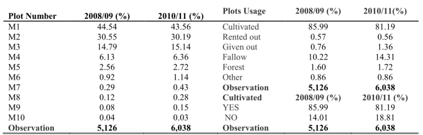
Table 1: Plot Usage in 2008/09 and 2010/11 NPS

Plot Number 2008/09 (%) 2010/11 (%) Plots Usage 2008/09 (%) 2010/11(%)

M1 44.54 43.56 Cultivated 85.99 81.19 M2 30.55 30.19 Rented out 0.57 0.56 M3 14.79 15.14 Given out 0.76 1.36 M4 6.13 6.36 Fallow 10.22 14.31 M5 2.56 2.72 Forest 1.60 1.72 M6 0.92 1.14 Other 0.86 0.86 M7 0.29 0.43 Observation 5,126 6,038 M8 0.12 0.28 Cultivated 2008/09 (%) 2010/11 (%) M9 0.08 0.15 YES 85.99 81.19 M10 0.04 0.03 NO 14.01 18.81 Observation 5,126 6,038 Observation 5,126 6,038

Note: Based on information reported by plot for the long season only.

Table 1 shows that just over 43 percent of farms had only one plot and over 90 percent of farms had three or fewer plots (in both surveys). Over 80 percent of plots were cultivated with 10-14 percent left fallow; the proportionally large increase in the share left fallow in 2010/11 deserves further investigation. There is no plots attrition between the 2008/09 and 2010/11, instead the plots increased by 912 (more than 17 percent of 2008/09 total). This is likely to be due to households’ splits that lead to new entrants acquiring new plots. Table 2 provides the distribution of farm size: over half of farms are one acre or less, more than 10 percent are two acres and less than 15 percent are four or more acres.

(12)

Table 2: Household Farm Size by Acre in 2008/09 and 2010/11 NPS

Acreage 2008/09 percent 2010/11 percent

< 0.50 12.38 13.89 0.50 15.65 13.24 1.00 25.72 20.39 1.50 8.02 7.36 1.75 0.18 0.56 2.00 12.49 11.12 2.50 2.76 3.45 3.00 7.10 4.86 3.50 0.54 1.1 4.00 4.76 3.35 4.50 0.26 0.39 5.00 2.70 2.89 > 5.00 7.57 6.05

Note: As for Table 1; based on adding up all plots for each farm.

Table 3: Distribution of Crops by Plots in 2008/09 and 2010/11 NPS

No. Crops 2008/09 2010/11 Freq. % Freq. % 1 Maize 1,608 38.99 2,044 42.36 2 Paddy 489 11.86 610 12.64 3 Sorghum 155 3.76 172 3.56 4 Millet 75 1.82 69 1.43 5 Wheat 19 0.46 18 0.37 6 Cassava 670 16.25 720 14.92 7 Irish Potatoes 30 0.73 25 0.52 8 Sweet Potatoes 107 2.59 102 2.11 9 Beans 205 4.97 189 3.92 10 Nuts, Seeds 199 4.83 142 2.94 11 Cotton 61 1.48 56 1.16 12 Tobacco 22 0.53 27 0.56 13 Pytherum - - 7 0.15 14 Sisal 3 0.07 3 0.06 15 Coffee 35 0.85 45 0.93 16 Tea 5 0.12 6 0.12 17 Cocoa 8 0.19 14 0.29 18 Cashew nuts 141 3.42 112 2.32 19 Sugarcane 20 0.48 19 0.39 20 Spices 9 0.22 15 0.31 21 Banana 174 4.22 293 6.07 22 Fruits 27 0.65 50 1.04 23 Vegetables 41 0.99 50 1.04 24 Others 21 0.51 37 0.77 Observation /Total 4,124 100 4,825 100

Note: As for Table 1; based on reported main crop planted on plot in the long season. The difference in sample between Table 1 and 2 are attributed to different files with different focus plots/crops.

(13)

Table 3 reports the distribution of crops by plot for the long season; cash crop production is understated as the separate information on permanent (tree) crops has not yet been incorporated into the summary tables. The figures for cash crops such as tobacco or coffee can be interpreted as relating only to plots where they are inter-cropped (the share of plots with cashew nuts is probably accurate). The major food crops (maize, paddy and cassava) are grown on more than two-thirds of all plots; sorghum, banana, nuts and seeds, beans, and sweet potatoes are also grown on significant numbers of plots. These shares refer only to the major crops grown on the plot; almost 60 percent of plots are inter-cropped (Table 4), often with more than two crops (the plot may be partitioned for separate crops; tree crops may be mixed, such as coffee and bananas; or food crops may be planted under trees).

Table 4 reports important characteristics of the farms. Over 80 percent of plots are owned by the farmer and up to 95 percent are owned or used with free access; renting accounts for about 5 percent of plots. Very few plots are irrigated, 3 percent or fewer, demonstrating that farming is almost always rain-fed; in this context it is unfortunate that farmers were not asked questions about the reliability of rainfall, quantity and timing, as in the Ethiopian surveys analysed in Abrar and Morrissey (2006). About 10 percent purchase inorganic fertilizer or pesticides (these are likely to be same farms) or use organic fertilizer (which may be different farms). Inconsistencies between the two surveys are evident: although the sample was larger in 2010/11, fewer answered questions on fertilizer use. Almost a third use improved seeds and also about a third employ hired labour.

One reason for the low use of purchased inputs is the high cost for farmers with low incomes (although not reported here, the NPS reports than only one or two per cent of farmers are able to obtain inputs on credit). Table 5 reports that almost two-thirds have loam soil and most others are either sandy or clay; about half report the soil is of good quality and 45 percent that it is average; less than 15 percent of plots suffer from erosion and more than half are flat, with about another third gently sloped. In sum, the majority of farms are small, owned, rain-fed with good soil and orientation but do not use purchased inputs (except perhaps for seeds and hired labour). An important issue to address in future analysis is the differences between those farms that purchase inputs (especially fertilizer) and those that do not. One would expect that only larger and/or more commercial farms are able to purchase inputs, and this may be related to the crops grown (and the availability of irrigation). For example, vegetables, beans and perhaps fruits should be relatively profitable and responsive

(14)

to fertilizer. However, as noted in Section 2, some producers of maize or paddy may be able to obtain fertilizer subsidies.

Table 4: Farming Characteristics 2008/09 and 2010/11 NPS

2008/09 2010/11

Ownership status Freq. Percent Cum. Freq. Percent Cum.

Owned 4,268 83.26 83.26 5,088 84.27 84.27

Used free of charge 567 11.06 94.32 698 11.56 95.83

Rented in 256 4.99 99.32 201 3.33 99.16

Kushirikiana 6 0.12 99.43 3 0.05 99.21

Shared - own 29 0.57 100 48 0.79 100

Total 5,126 100 6,038 100

Plot Irrigated Freq Percent Cum. Freq Percent Cum.

Yes 108 2.54 2.54 103 2.06 2.06

No 4,144 97.46 100.00 4,886 97.94 100

Total 4,252 100 4,989 100

Plot Intercropped Freq. Percent Cum. Freq. Percent Cum.

Yes 3,298 63.56 63.56 3,886 64.76 64.76

No 1,891 36.44 100 2,115 35.24 100

Total 5,189 100 6,001 100

Organic Fertilizer Freq. Percent Cum. Freq. Percent Cum.

Yes 446 10.66 10.66 513 10.68 10.68

No 3,738 89.34 100 4,292 89.32 100

Total 4,184 100 4,805 100

Inorganic Fertilizers Freq. Percent Cum. Freq. Percent Cum.

Yes 456 10.90 10.90 615 12.80 12.80

No 3,729 89.10 100 4,190 87.20 100

Total 4,185 100 4,805 100

Pesticides Freq. Percent Cum. Freq. Percent Cum.

Yes 450 10.75 10.75 433 9.01 9.01

No 3,735 89.25 100 4,372 90.99 100

Total 4,185 100 4,805 100

Improved Seeds Freq. Percent Cum. Freq. Percent Cum.

Yes 1,690 29.79 29.79 1,524 25.41 25.41

No 3,983 70.21 100 4,474 74.59 100

Total 5,673 100 5,998 100

Hired Labour Freq. Percent Cum. Freq. Percent Cum.

Yes 1,302 31.14 31.14 1,299 27.03 27.03

No 2,879 68.86 100 3,506 72.97 100

Total 4,181 100 4,805 100

Note: As for Table 1; based on reported main crop planted on plot in the long season; table reports frequency (Freq), percentage and cumulative percentage (cum).

(15)

Table 5: Soil and Land Quality 2008/09 and 2010/11 NPS

2008/09 2010/11

Type of Soil Freq. Percent Cum. Freq. Percent Cum.

Sandy 895 21.04 21.04 984 19.72 19.72

Loam 2,625 61.72 82.77 3,043 60.98 80.70

Clay 640 15.05 97.81 891 17.86 98.56

Other 93 2.19 100.00 72 1.44 100

Total 4,253 100 4,990 100

Quality of the Soil Freq. Percent Cum. Freq. Percent Cum.

Good 2,143 50.39 50.39 2,315 46.40 46.40

Average 1,884 44.30 94.69 2,336 46.82 93.23

Bad 226 5.31 100 338 6.77 100

Total 4,253 100 4,989 100

Erosion Problem Freq. Percent Cum. Freq. Percent Cum.

Yes 555 13.05 13.05 644 12.91 12.91

No 3,697 86.95 100.00 4,345 87.09 100

Total 4,252 100 4,989 100

Measures taken Freq. Percent Cum. Freq. Percent Cum.

Yes 659 15.50 15.50 511 10.24 10.24

No 3,593 84.50 100 4,477 89.74 100

Total 4,252 100 4,989 100.

Steep slope Freq. Percent Cum. Freq. Percent Cum.

Flat bottom 2,176 51.19 51.19 2,941 58.95 58.95

Flat top 502 11.81 63.00 332 6.65 65.60

Slightly sloped 1,414 33.26 96.26 1,501 30.09 95.69

Very steep 159 3.74 100 215 4.31 100

Total 4,251 100 4,989 100

Note: As for Table 4.

The remaining tables provide summary data on the 24 main crops (and on ‘others’ category) for 8 regions (some 7 aggregated from the 21 regions in Mainland Tanzania and 1 from the 5 regions in Zanzibar). For convenience we limit the discussion to median values for 2010/11 but where relevant will refer to mean values and statistics for 2008/09 (all in Appendix Tables). As there is considerable variability in farm and plot size, the median is a better indication of the ‘norm’ for the average farm (and is typically considerably lower than the mean). The simple pattern is one of significant variation across regions for every crop, although every region has at least one productive crop (and often a crop for which it is the most productive region).

(16)

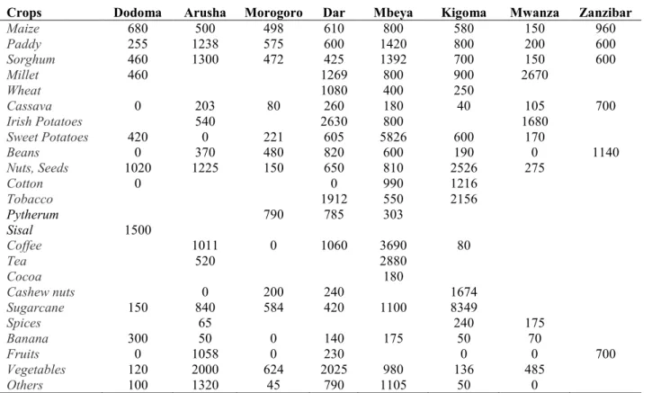
Table 6 reports the median harvest in kg/farm. For the major crop, maize, Zanzibar, Mbeya and Dodoma have the highest median production (Arusha, Morogoro and Dodoma have highest mean production), whereas for paddy Mbeya, Arusha, Kigoma and Morogoro have the highest median values. Zanzibar, Dar and Mbeya have the highest values for cassava; Dar is also high for Irish potatoes (with Mwanza and Mbeya) and beans (with Mbeya and Zanzibar). Cashew nuts are mainly grown in Morogoro, Dar and Kigoma, sugarcane in Dodoma, Arusha, Morogoro, Dar, Mbeya and Kigoma, and banana is grown mostly in same regions including Mwanza. Fruits are mostly grown in Arusha, Morogoro, Dar and Zanzibar, and vegetables in every region except for Mwanza. Regions with the highest median quantity do not always have (among) the highest mean quantity, although in general the broad rankings are similar or consistent (Table A3).

(17)

Table 6: Median Quantity by Harvested Crop (Kg/farm) by Region 2010/11 NPS

Crops Dodoma Arusha Morogoro Dar Mbeya Kigoma Mwanza Zanzibar

Maize 680 500 498 610 800 580 150 960 Paddy 255 1238 575 600 1420 800 200 600 Sorghum 460 1300 472 425 1392 700 150 600 Millet 460 1269 800 900 2670 Wheat 1080 400 250 Cassava 0 203 80 260 180 40 105 700 Irish Potatoes 540 2630 800 1680 Sweet Potatoes 420 0 221 605 5826 600 170 Beans 0 370 480 820 600 190 0 1140 Nuts, Seeds 1020 1225 150 650 810 2526 275 Cotton 0 0 990 1216 Tobacco 1912 550 2156 Pytherum 790 785 303 Sisal 1500 Coffee 1011 0 1060 3690 80 Tea 520 2880 Cocoa 180 Cashew nuts 0 200 240 1674 Sugarcane 150 840 584 420 1100 8349 Spices 65 240 175 Banana 300 50 0 140 175 50 70 Fruits 0 1058 0 230 0 0 700 Vegetables 120 2000 624 2025 980 136 485 Others 100 1320 45 790 1105 50 0

Note: Based on crop/farm data in 2010/11 NPS. The 21 regions identified in the NPS for Mainland Tanzania and 5 regions identified for Zanzibar are combined into regions as listed here (see Appendix Table A1).

Unit values vary across regions so the rankings in terms of value of output per plot (Table 7) are not always identical to those for quantity. For maize, Zanzibar, Dar, Mbeya and Dodoma have high value but Dodoma (not Dar) has the highest median value, whereas for paddy Arusha, Mbeya, Kigoma and Morogoro remain with the highest median values. Zanzibar, Dar and Mbeya again have the highest values for cassava; Dar is also the highest value for Irish potatoes (with Mwanza and Mbeya as before) and Zanzibar is again highest for beans (followed by Dar, Mbeya and Morogoro). Cashew nuts are mainly grown in Kigoma, Morogoro and Dar, sugarcane in Kigoma, Mbeya, Arusha and Morogoro, banana is grown mostly in same regions including Mwanza, fruits in Arusha, Zanzibar and Dar, and vegetables in all regions except Mwanza and Zanzibar; in all these cases the regions also have the highest median values. Regions with the highest median quantity do not always have (among) the highest mean quantity, although in general the broad rankings are similar or consistent (Table A3).

(18)

Table 7: Median Value Harvested Crop (000’ TShs/farm) by Region 2010/11 NPS

Note: Based on crop/farm data in 2010/11 NPS.

As plot sizes may vary by region it is more informative to examine yields (kg/acre, in Table 8), income per acre (Table 9) and ‘profit’ (income minus purchased inputs) per acre (Table 10). As purchased inputs are report at the plot level and have to be allocated to crops, as most plots have more than one crop, the profit estimates may be unreliable (especially as answers for apportioning crops to plots are not always consistent). In general the ‘ranking’ of regions is unaltered. For maize (Zanzibar, Mwanza, Dodoma and Arusha) and for paddy (Arusha, Kigoma, Mbeya and Dodoma) the same regions have the highest yield, income and profit. Dodoma, Arusha, Morogoro and Mwanza have the highest yields and incomes for cassava; Mbeya and Dar have the highest yield and income for Irish potatoes (with Arusha, which appears to have far higher profit) and Mbeya, Mwanza and Dar have highest for beans (although a number of regions appear to have similar profits).

(19)

Table 8: Median Crop Yield (kg/acre) by Region 2010/11 NPS

Maize 330 300 237 213 255 208 350 480 Paddy 330 909 275 300 360 400 235 150 Sorghum 164 650 216 180 192 136 269 150 Millet 182 333 182 100 763 Wheat 390 541 46 Cassava 355 350 226 187 200 199 210 140 Irish Potatoes 308 1533 3200 560 Sweet Potatoes 667 1500 388 293 544 400 350 Beans 135 211 199 229 275 150 270 253 Nuts, Seeds 160 411 194 168 300 151 141 Cotton 125 176 132 Tobacco 283 550 329 Pytherum 790 209 223 Sisal 710 Coffee 407 200 397 688 296 Tea 558 2880 Cocoa 550 Cashew nuts 384 160 431 Sugarcane 150 420 389 280 437 1868 Spices 325 480 175 Banana 286 230 130 280 202 144 269 Fruits 276 142 173 320 140 Vegetables 120 533 210 409 571 272 373 Others 240 660 267 675 321 100 350

Table 9: Median Crop Income (000’ TShs/acre) by Regions 2010/11 NPS

(20)

Table 10: Median Profit (000’ TShs/acre) by Regions 2010/11 NPS

Maize 141 119 82 80 90 71 150 108 Paddy 153 354 135 129 144 183 167 37 Sorghum 54 115 74 74 48 63 145 43 Millet 51 88 66 5 224 Wheat 93 89 21 Cassava 132 128 85 72 82 68 152 41 Irish Potatoes 150 203 93 21 Sweet Potatoes 223 159 136 117 103 117 288 Beans 74 57 103 75 89 56 255 29 Nuts, Seeds 90 148 198 88 87 119 128 Cotton 43 64 93 Tobacco 373 960 248 Pytherum 218 51 81 Sisal 144 Coffee 88 46 79 124 24 Tea 151 18 Cocoa 159 Cashew nuts 135 77 89 Sugarcane 75 116 121 92 106 562 Spices 134 46 Banana 135 127 59 64 115 44 212 Fruits 73 52 72 216 41 Vegetables 305 209 175 556 169 63 167 Others 130 271 170 122 34 20 175

Cashew nuts are mainly grown in Morogoro and Dar, and sugarcane in Kigoma, Morogoro, Mbeya, Arusha, Dodoma and Dar. Although banana has highest production and in Dodoma, Mbeya and Dar and profit in Mwanza, Dodoma, Arusha and Mbeya, yield and income are highest in Dodoma, Dar and Mwanza. Fruits production and profit is highest in Mwanza, but yield and income is highest in Arusha and Mwanza. Vegetables production, yield and income is highest in Mbeya, Arusha, Dar and Mwanza, profit are higher in Dar, Arusha and Dodoma.

Three general conclusions can be drawn. First, we can be quite confident in identifying which crops are most important in which regions and vice versa, although it is not a one to one correspondence (many regions are important for a number of crops, and most crops are grown productively in a number of regions) and high production quantities and values do not necessarily imply high yield and income per acre. Second, the NPS data require further careful checking before proceeding to econometric analysis. The problem in deriving a measure of ‘profit’ has been shown, and apparent inconsistencies between farm and acre level measures have to be investigated. Furthermore, if results for 2008/09 (Appendix tables)

(21)

are compared to 2010/11 there are apparently inconsistent changes in magnitudes and rankings across crops and regions. Third, and following, careful checking of the data measured at the farm level will be required before embarking on econometric analysis. Although ‘adding up’ the plots in a farm is easy, the difficulty arises in determining the actual acreage devoted to each crop when more than one crop is grown on a plot (as is common) as the information reported is only approximate. This creates a particular problem in allocating purchased inputs (reported at the plot level) to crops. Furthermore, permanent and short season crops have to be included to accurately capture farm output and income. However, having undertaken this scoping investigation of the data it is evident that analysis of productivity and supply response is feasible.

5 Conclusion: Productivity and Supply Response

Although the NPS are small in sample size (3,280 households), they provide recent farm level household panel data with two waves (so lagged prices are available) and econometric analysis is feasible. The first preliminary analysis would be of the determinants of yields at the crop/farm level. This would employ variables subsequently used in analysing supply response as yield is posited to be a function of land size and quality, fertilizer and pesticide use, irrigation (unfortunately data on adequacy of rain was not collected) and farmer characteristics (age, education). We do not propose to estimate technical efficiency, but could as a final stage estimate supply response incorporating efficiency following the method employed by Abrar and Morrissey (2006).

The core analysis will be of supply response, the price and non-price factors determining production and how responsive farmers are to these factors. Two fundamental approaches are used in studying production decisions: the production function (primal approach) and the profit function (dual approach). Under appropriate regularity conditions, and with the assumption of profit maximization, both functions contain the same essential information on a production technology. The dual approach has several advantages: prices are specified as the exogenous variables as opposed to input quantities (prices are usually less collinear than input quantities); estimates of output supply, input demand, and the price (and cross-price) elasticities are more easily derived (as derivatives of the profit function); and it is more flexible for modelling multiple outputs and inputs systems (as is the case here).

(22)

(4) Following Abrar et al. (2004) a profit, cost, or revenue function is estimated employing a variant specification of the profit function. Assume that farmers attempt to maximise restricted profit, defined as the return to the variable factors, so the profit maximisation problem can be expressed as:

Max Π (p,w;z) = Ma x p'y – r'x (1) s.t. F(y, x; z) ≤ 0,

where Π , p, w, respectively, represent restricted profit, and vectors of output and input prices. The variables y and x represent vector of output and input quantities respectively. F(.) is the production technology set of the producer, and Z is a set of control variables. The restricted profit function represents the maximum profit the farmer could obtain with available prices, fixed factors, and production technology. The profit-maximising output supply and input demand functions are derived as:

(

)

m m P z w p z w p Y ∂ Π ∂ = , ; ) ; , ( , ∀ m=1,...,M, (2) and

(

)

n n W z w p z w p X ∂ Π ∂ = − ( , ; ) , ; , ∀ n=1,...,N. (3)

where m and n index the outputs and variable inputs respectively. There are usually four (translog, generalised Leontief, generalised Cobb-Douglas, and the quadratic forms) functional forms of the profit function that have been used in the literature. A choice of a particular specification, in part, depends on the nature of the data set available, and the translog profit function is generally preferred. These estimated parameters can be used to derive the elasticities for production relations of multiple-input, multiple-output farms.

The Translog profit function can be specified as:

𝑙𝑛𝜋∗₍_𝑝_,_𝑤_,_𝑧_;_𝛽_{) =}_𝛽

0+∑ 𝛽𝑖 𝑖ln(Pi∗) +∑ 𝛽𝑣 𝑣lnWv∗+∑ 𝛽𝑚 𝑚lnZm+

∑ ∑ βi v ivln(Pi∗) lnWv∗+∑ ∑ βi m imln(Pi∗) lnZm+∑ ∑ βv m vmlnWv∗ lnZm

(23)

+1₂��∑ ∑ βi j ijln(Pi∗)ln�Pj∗�+∑ ∑ βv r vrlnWv∗lnWr∗+∑ ∑ βm k mklnZmlnZk��+𝑒

where

π* = restricted variable profit, normalized by the price of labour *

*_,

j i P

P _{= Price of outputs, respectively, normalized by the price of labour} *

*_,

r v W

W _{= Price inputs, respectively, normalized by the price of labour}

Z = quantity of fixed and quasi-fixed inputs (land size, family labour, animal capital) and other farmer social-demographic and human capital factors (age, education and farming experience).

The βs are parameters to be estimated and ε is an error term with the usual properties. All prices are normalized by the price of labour. The core variables to be derived from the NPS are summarized in Table 11.

Table 11: Summary of variables to be used (measured farm-level by crop)

Variable Category Variable Name/Symbol Description/Measurement

Profit Restricted farmer profit (π*₎ _{Total revenue less cost of variable inputs}

(purchased inputs plus hired labour) Prices of Outputs _{Output price (} *_, *

j i P

P ) Unit price of crop sales Prices of Inputs _{Input Price (} *_, *

r v W

W ) Prices of variable inputs Fixed/quasi fixed (Z) Land Size Total area cultivated in acres

Family Labour Total own labour available to the household, between the ages 15 and 65 inclusive

Animal Capital Total number of hooved animals available to a farming household

Control Variables Age Farmer age in years *

Education Farmer formal education in years Irrigation Binary variable (yes = 1)

Soil quality Index combining indicators Market access Distance to nearest market/village

Notes: Age is used (*) on assumption that farmer has always been in farming. If there is information on those only recently in farming or who took a break, years of experience in farming may be included as a separate variable. Information on land and soil quality for plots will be used to construct binary variables [Good = 1, Poor =0] (at farm level) combining soil erosion [Yes = 0, No =1], are there control measures [Yes = 1, No =0], soil type and land slope categories converted to [1, 0].

(24)

References

Abrar, S., O. Morrissey and A. Rayner (2004), ‘Crop-level Supply Response by Agro-climatic Regions in Ethiopia’ Journal of Agricultural Economics, 55:2, 289-312

Abrar, S., and O. Morrissey (2006), ‘Supply Response in Ethiopia: Accounting for Technical Inefficiency’ Agricultural Economics, 35 (3), 303-317

Ahmed, S., Diffenbaugh, N., Hertel, T. and Martin, J. (2012), Agriculture and Trade Opportunities for Tanzania: Past Volatility and Future Climate Change, Review of Development Economics, 16 (3), 429-447

Anderson, K., W. Martin, D. Sandri and E. Valenzuela (2006), Methodology for Measuring Distortions to Agricultural Incentives, Agricultural Distortions Research Project Working Paper 02, World Bank, Washington DC, August.

Anderson, K. and W. Masters (eds, 2009), Distortions to Agricultural Incentives in Africa, Washington DC: World Bank

Arndt, C., Farmer, W., Strzepek, K. and Thurlow, J. (2012), Climate Change, Agriculture and Food Security in Tanzania, Review of Development Economics, 16 (3), 378-393 Fan, S., Nyange, D. and Rao, N. (2012), Public Investment and Poverty Reduction in

Tanzania: Evidence from Household Survey Data, Chapter 6 in T. Mogues and S. Benin (eds), Public Expenditures for Agriculture and Rural Development in Africa, London: Routledge, pp 154-177

Isinika, A., G. Ashimogo and J. Mlangwa (2005), From Ujamaa to Structural Adjustment – Agricultural Intensification in Tanzania, in G. Djurfeldt, H. Holmén, M. Jirström and R. Larsson (eds), The African Food Crisis: Lessons from the Asian Green Revolution, Wallingford: CABI Publications.

McKay, A., O. Morrissey and C. Vaillant (1999), ‘Aggregate Agricultural Supply Response in Tanzania’, J. International Trade and Economic Development, 8:1, 107-123

Morrissey, O. and V. Leyaro (2009), ‘Distortions to Agricultural Incentives in Tanzania’, in K. Anderson and W. Masters (eds.), chapter 11, pp. 307-328

Skarstein, R. (2005), Economic Liberalisation and Smallholder Productivity in Tanzania: From Promised Success to Real failure, 1985-1998, Journal of Agrarian Change, 5 (3), 334-362.

World Bank (1994), Tanzania Agriculture: A Joint Study by the Government of Tanzania and the World Bank, Washington DC: The World Bank

World Bank (2006), Tanzania: Sustaining and Sharing Economic Growth, Country Economic Memorandum and Poverty Assessment, Volume 1 (draft, 28 April).

(25)

Appendix A: Supplementary Tables

Table A1: Correspondence of the 10 to the 21 regions in Tanzania

No. Region name Comprises Ecological zone

1 Dodoma Dodoma, Singida, Tabora, Shinyanga 2 Arusha Arusha, Kilimanjaro, Manyara

3 Morogoro Morogoro,Tanga, Coast, Lindi, Mtwara 4 Dar es Salaam Dar es Salaam,

5 Mbeya Mbeya, Ruvuma, Iringa

6 Kigoma Kigoma, Rukwa

7 Mwanza Mwanza, Mara, Kagera

8 Zanzibar

North Unguja, South Unguja, West Unguja, North Pemba, South Pemba

Source: Authors own compilation

Table A2: Weather Condition at GPS Measurement: 2010/11 NPS

Climatic Zones Freq. Percent Cum.

Clear/Sunny 3,953 34.07 34.07

Mostly Clear/Mostly Sunny 1,422 12.26 46.33 Partly Cloudy/Partly Sunny 5,038 43.42 89.75 Mostly Cloudy/Considerable Cloudiness 592 5.10 94.85

Completely Cloudy 398 3.43 98.28

Rainy 199 1.72 100.00

Total 11,602 100

Source: Authors own compilation

Table A3: Mean Quantity of Harvested Crops by Regions 2010/11 NPS

Note: Mean in kg per farm based on 2010/11 NPS.

(26)

Table A3: Mean Value of Harvested Crop (000’ TShs/plot) by Regions 2010/11 NPS

Note: Mean in thousand (000’) TShs per farm based on 2010/11 NPS.

Table A4: Mean Crop Yield (Kg/Acre) by Regions 2010/11 NPS

Note: Yield in Kg per acre based on 2010/11 NPS.

(27)

Table A5: Mean Crop Income (000’ TShs/acre) by Regions 2010/11 NPS

Note: Mean in thousand (000’) TShs per acre based on 2010/11 NPS.

Table 6: Mean Profit in ‘000’TSHs by Regions: 2010/11 NPS

Maize 141 119 82 80 90 71 150 108 Paddy 153 354 135 129 144 183 167 37 Sorghum 54 115 74 74 48 63 145 43 Millet 51 88 66 5 224 Wheat 93 89 21 Cassava 132 128 85 72 82 68 152 41 Irish Potatoes 150 203 93 21 Sweet Potatoes 223 159 136 117 103 117 288 Beans 74 57 103 75 89 56 255 29 Nuts, Seeds 90 148 198 88 87 119 128 Cotton 43 64 93 Tobacco 373 960 248 Pytherum 218 51 81 Sisal 144 Coffee 88 46 79 124 24 Tea 151 18 Cocoa 159 Cashew nuts 135 77 89 Sugarcane 75 116 121 92 106 562 Spices 134 46 Banana 135 127 59 64 115 44 212 Fruits 73 52 72 216 41 Vegetables 305 209 175 556 169 63 167 Others 130 271 170 122 34 20 175

Note: Mean in thousand (000’) TShs per acre based on 2010/11 NPS.

(28)

Table A7: Mean Quantity of Harvested Crop (Kg/farm) by Regions 2008/09 NPS

Crops Dodoma Arusha Morogoro Dar Mbeya Kigoma

Maize 1042 960 978 1090 2399 705 Paddy 1018 793 957 1006 1897 1105 Sorghum 1117 81 862 920 1949 507 Millet 961 102 1133 814 351 Wheat 1435 Cassava 0 1993 680 1274 427 Irish Potatoes 1591 1043 1482 260 Sweet Potatoes 500 766 743 717 1108 983 Beans 1355 565 889 1430 1754 723 Nuts, Seeds 1307 557 439 1221 1777 478 Cotton 2126 338 Tobacco 1319 1421 Sisal 1136 Coffee 380 Cashew nuts 3886 161 3160 Sugarcane 525 Banana 754 454 522 Fruits 300 492 184 4050 Vegetables 470 852 3218 1350 2221 1171 Others 286 7674 444

Table A8: Median Quantity of Harvested Crop (Kg/farm) by Region 2008/09 NPS

Note: Median in kg per farm based on 2008/09 NPS.

(29)

Table A9: Mean Value of Harvested Crop (000’ TShs/farm) by Regions 2008/09 NPS

Table A10: Median Value of Harvested Crop (000’ TShs/farm) by Regions 2008/09 NPS

Note: Median in thousand (000’) TShs per plot based on 2008/09 NPS.

(30)

Table A11: Mean Crop Yield (Kg/acre) by Region 2008/09 NPS

Maize 275 476 380 450 3312 380 Paddy 437 593 881 300 431 1129 Sorghum 286 144 318 320 508 392 Millet 226 78 456 303 483 Wheat 301 Cassava 405 355 203 571 Irish Potatoes 713 262 240 824 Sweet Potatoes 100 874 390 250 438 313 Beans 222 315 301 464 395 441 Nuts, Seeds 254 400 373 443 419 487 Cotton 434 246 Tobacco 699 287 Sisal 327 Coffee 253 Cashew nuts 1421 161 181 Sugarcane 105 Banana 355 198 567 Fruits 300 98 92 900 Vegetables 121 537 719 474 413 394 Others 291 691 90

Note: Yield in Kg per acre based on 2008/09 NPS

Table A11: Median Crop Yield (Kg/acre) by Region 2008/09 NPS

Note: Based on crop/acre data in 2010/11 NPS.

(31)

. Table A12: Mean Crop Income (000 TShs/acre) by Region 2008/09 NPS

Note: Based on crop/acre data in 2010/11 NPS.

Table A12: Median Crop Income (000 TShs/acre) by Region 2008/09 NPS

Note: Median in thousand (000’) TShs per acre based on 2008/09 NPS.

(32)

Table A13: Mean Profit (000’TShs/acre) by Regions 2008/09 NPS

Maize 46 117 95 112 94 123 Paddy 116 207 223 70 118 112 Sorghum 47 75 113 57 158 97 Millet 40 34 96 67 114 Wheat 79 Cassava 78 53 22 179 Irish Potatoes 116 66 55 104 Sweet Potatoes 8 118 95 63 79 153 Beans 42 96 68 105 89 130 Nuts, Seeds 50 63 130 95 76 138 Cotton 102 57 Tobacco 87 85 Sisal 50 Coffee 51 Cashew nuts 110 28 26 Sugarcane 296 Banana 61 43 158 Fruits 42 15 299 Vegetables 22 131 118 102 269 139 Others 71 67 83

Table A13: Median Profit (000’TShs/acre) by Regions 2008/09 NPS

Maize 34 80 57 53 53 71 Paddy 108 71 59 45 133 89 Sorghum 36 94 50 28 53 51 Millet 38 28 62 39 126 Wheat 62 Cassava 53 43 22 83 Irish Potatoes 192 38 34 120 Sweet Potatoes 8 30 24 46 60 48 Beans 46 63 46 67 57 52 Nuts, Seeds 40 23 56 58 49 81 Cotton 82 45 Tobacco 25 45 Sisal 46 Coffee 51 Cashew nuts 74 28 26 Sugarcane 296 Banana 40 27 126 Fruits 32 15 299 Vegetables 22 96 64 57 55 84 Others 90 12 56