Dissertations Theses and Dissertations
Fall 2012
The goodness-of-fit tests for geometric models
Feiyan Chen
New Jersey Institute of Technology
Follow this and additional works at:https://digitalcommons.njit.edu/dissertations Part of theMathematics Commons
This Dissertation is brought to you for free and open access by the Theses and Dissertations at Digital Commons @ NJIT. It has been accepted for inclusion in Dissertations by an authorized administrator of Digital Commons @ NJIT. For more information, please contact
digitalcommons@njit.edu.
Recommended Citation
Chen, Feiyan, "The goodness-of-fit tests for geometric models" (2012).Dissertations. 350.
Copyright Warning & Restrictions
The copyright law of the United States (Title 17, United
States Code) governs the making of photocopies or other
reproductions of copyrighted material.
Under certain conditions specified in the law, libraries and
archives are authorized to furnish a photocopy or other
reproduction. One of these specified conditions is that the
photocopy or reproduction is not to be “used for any
purpose other than private study, scholarship, or research.”
If a, user makes a request for, or later uses, a photocopy or
reproduction for purposes in excess of “fair use” that user
may be liable for copyright infringement,
This institution reserves the right to refuse to accept a
copying order if, in its judgment, fulfillment of the order
would involve violation of copyright law.
Please Note: The author retains the copyright while the
New Jersey Institute of Technology reserves the right to
distribute this thesis or dissertation
Printing note: If you do not wish to print this page, then select
“Pages from: first page # to: last page #” on the print dialog screen
The Van Houten library has removed some of the
personal information and all signatures from the
approval page and biographical sketches of theses
and dissertations in order to protect the identity of
NJIT graduates and faculty.
ABSTRACT
THE GOODNESS-OF-FIT TESTS FOR GEOMETRIC MODELS by
Feiyan Chen
We propose two types of goodness-of-fit tests for geometric distribution and for a bivariate geometric distribution called BGD(B&D), based on their probability generating function (PGF). The first type is a special-case application of the general testing procedure for discrete distributions proposed by Kocherlakota and Kocherlakota (1986). The second type utilizes the supremum of the absolute value of the standardized difference between the PGF’s maximum likelihood estimator (MLE) and its empirical counterpart as the test statistic. We verify the asymptotic properties of the test statistics for the first type of test and explore the asymptotic behaviors of the test statistics for the second type of test by calculating the empirical critical points and constructing the density curves. We compare the proposed tests with Chi-square and the empirical distribution function (EDF) related tests proposed in the literature in terms of significance level and power. Based on the comparison results, we recommend the second type of goodness-of fit test for both geometric distribution and BGD(B&D) because of its robustness, efficiency in computation and no need for selectingt. Real data sets are used for illustration.
by Feiyan Chen
A Dissertation
Submitted to the Faculty of
New Jersey Institute of Technology and
Rutgers, The State University of New Jersey – Newark in Partial Fulfillment of the Requirements for the Degree of
Doctor of Philosophy in Mathematical Sciences Department of Mathematical Sciences, NJIT
Department of Mathematics and Computer Science, Rutgers-Newark January 2013
Copyright c° 2013 by Feiyan Chen ALL RIGHTS RESERVED
THE GOODNESS-OF-FIT TESTS FOR GEOMETRIC MODELS Feiyan Chen
Sunil K. Dhar, PhD, Dissertation Advisor Date
Associate Professor, Department of Mathematical Sciences, NJIT
Sundarraman Subramanian, PhD, Committee Member Date
Associate Professor, Department of Mathematical Sciences, NJIT
Aridaman K. Jain, PhD, Committee Member Date
Senior University Lecturer, Department of Mathematical Sciences, NJIT
Wenge Guo, PhD, Committee Member Date
Assistant Professor, Department of Mathematical Sciences, NJIT
Ganesh K. Subramanian, PhD, Committee Member Date
BIOGRAPHICAL SKETCH
Author: Feiyan Chen
Degree: Doctor of Philosophy
Date: January 2013
Undergraduate and Graduate Education:
• Doctor of Philosophy in Mathematical Sciences, New Jersey Institute of Technology, Newark, NJ, 2013
• Master of Applied Statistics,
New Jersey Institute of Technology, Newark, NJ, 2009
• Master of Computer Sciences,
Xi’an Jiaotong University, Xi’an, China, 2005
• Bachelor of Computer Sciences,
Xi’an Polytechnic University, Xi’an, China, 2002
Major: Mathematical Sciences
Presentations and Publications:
Feiyan Chen, “Probability Generating Function based Goodness-of-fit Tests for Geometric Distribution,” 57th Annual Meeting of New Jersey Academy of Science , Seton Hall University, South Orange, April 21, 2012.
Feiyan Chen, “Comparison of Goodness-of-fit Tests for Geometric models,” the Ninth Annual
Conference on Frontiers in Applied and Computational Mathematics (FACM ’12) ,
Department of Mathematical Sciences, NJIT, May 18-20, 2012.
Feiyan Chen, “Numerical Study of the Goodness-of-fit Tests for Geometric Models,” Applied
Mathematics Seminar, Department of Mathematical Sciences, NJIT, June 18, 2012.
Feiyan Chen, “The Goodness-of-fit Tests for BGD(B&D),” VIIIth Annual Graduate Student
Research Day, NJIT, November 12, 2012.
lies opportunity.
—Albert Einstein
ACKNOWLEDGMENT
First of all, I would like to thank my dissertation advisor, Dr. Sunil K. Dhar for his tremendous guidance with this dissertation. Ever since I joined the PhD program of the Department of Mathematical Sciences in NJIT, he has been a steadfast source of information, ideas, support, and energy. I am deeply grateful for the patient, encouraging and resourceful guidance he has been giving me throughout the last few years, and I sincerely wish for him all the best in all his future endeavors.
I also would like to extend my gratitude to the other members in my committee for their kind encouragement and support to me throughout all these years while I was in the graduate school as well as throughout the process of working on my dissertation: Dr. Sundarraman Subramanian, Dr. Aridaman K Jain, Dr. Wenge Guo, and Dr. Ganesh K Subramanian. I would like to thank Professor Jonathan H. Luke, Chair of the Department of Mathematical Sciences, for his support.
I also want to thank all the other faculty, staff members and graduate students in the Department of Mathematical Sciences for all the help they have been giving me in the last four years. It has been a great honor to me to get to know all of them.
Last, but not the least, I would like to give the most sincere gratitude to my beloved husband, Peixin Zhang and my adorable son, Eric Zhang. While all has been encouraging and enlightening, I simply would not have accomplished even a little bit without the love, support and understanding from my family.
Chapter Page
1 INTRODUCTION . . . . 1
2 REVIEW OF BACKGROUND . . . . 5
2.1 Chi-square Tests for Geometric Models . . . . 5
2.2 EDF based Tests for Geometric Models . . . . 6
2.3 K & K Method of Goodness-of-fit Tests . . . . 7
3 TEST STATISTICS . . . . 10
3.1 Goodness-of-fit Tests for Geometric Distribution . . . . 10
3.1.1 K&K Method with Singlet . . . . 10
3.1.2 K&K Method with Multiplet’s . . . . 11
3.1.3 Supremum Test based on PGF . . . . 12
3.2 Goodness-of-fit Tests for BGD(B&D) . . . . 13
3.2.1 K&K Method with Singlet . . . . 13
3.2.2 K&K Method with Multiplet’s . . . . 14
3.2.3 Supremum Test based on PGF . . . . 15
4 SIMULATION STUDY FOR TESTING GEOMETRIC DISTRIBUTION . . . . . 16
4.1 Empirical Distributions of Test Statistics . . . . 16
4.2 Evaluating Tests by Comparison . . . . 19
4.3 Real Example Analysis . . . . 26
5 SIMULATION STUDY FOR TESTING BGD(B&D) . . . . 28
5.1 Empirical Distribution of Test Statistics. . . . 28
5.2 Evaluating Tests by Comparison . . . . 36
5.3 Robustness Study . . . . 47
5.4 Remarks . . . . 50
5.5 Real Example Analysis . . . . 51
6 CONCLUSIONS . . . . 53
APPENDIX BGD(B&D) . . . . 54
REFERENCES . . . . 56
LIST OF TABLES
Table Page
4.1 Empirical Critical Points ofTq(t) based on 10,000 Replications . . . . 17
4.2 Empirical Critical Points ofSDn based on 10,000 Bootstrap Samples. . . . 19
4.3 Empirical (Theoretical) Critical Points ofχ2 cl1,χ2cl2andχ2cl3based on 10,000 Replications 20 4.4 Empirical Critical Points ofKS and ADwith n= 50 based on 10,000 Replications . 21 4.5 Powers(%) for Geometric Tests withp = 0.25 atα= 0.05 based on 10,000 Samples of Size n= 50 and the Mean of the Alternative is 4 . . . . 22
4.6 Powers(%) for Geometric Tests with p = 0.5 atα = 0.05 based on 10,000 Samples of Size n= 50 and the Mean of the Alternative is 2 . . . . 23
4.7 Powers(%) for Geometric Tests with p = 0.6 atα = 0.05 based on 10,000 Samples of Size n= 50 and the Mean of the Alternative is 5/3 . . . . 24
4.8 Library Circulation . . . . 26
4.9 Goodness-of-fit Tests Results based on the Real Data . . . . 27
5.1 MZ(t) Tests . . . . 28
5.2 MTq(t) Tests . . . . 31
5.3 Empirical Critical Points ofMSDn based on 10,000 Replications. . . . 35
5.4 Notations of Alternative Distributions. . . . 38
5.5 Empirical Critical Points ofMχ2 cl1 and Mχ2cl2 based on 10,000 Replications . . . . . 39
5.6 Empirical Critical Points ofMKS based on 10,000 Replications . . . . 39
5.7 Empirical Type I Error Rates (%) of MSDn, MKS, Mχcl21 and Mχ2cl2 at α = 5% based on 10,000 Replications . . . . 41
5.8 Powers(%) of Tests for BGD(B&D) withp= (0.8, 0.7, 0.9) atα= 0.05 based on 10,000 Replications . . . . 45
5.9 Powers(%) of Tests for BGD(B&D) withp = (0.50, 0.55, 0.45) at α = 0.05 based on 10,000 Replications . . . . 46
5.10 Powers (%) of Tests for BGD(B&D) withp = (0.64, 0.56, 0.86) atα = 0.05 . . . . . 49
5.11 Accidents Records of 122 Shunters during 1937-1947 . . . . 51
5.12 Statistic Values and P-values for Accident Records Example . . . . 52
Figure Page
4.1 Empirical percentiles ofZ(t) which is on the x-axis indicated byt value with n = 50 and p = 0.25. . . . . 16 4.2 Density curves ofSDn with various pand n. . . . . 18
4.3 Empirical Type I error rates ofSDn,KS and AD boxplots comparison. . . . . 25
5.1 Empirical percentiles ofMZ(t), which is identified by the subscript ofton the x-axis, forp = (0.8, 0.9, 0.7). . . . . 29 5.2 Empirical percentiles ofMZ(t), which is identified by the subscript ofton the x-axis,
forp = (0.50, 0.55, 0.45). . . . . 30 5.3 Empirical percentiles ofMZ(t), which is identified by the subscript ofton the x-axis,
forp = (0.25, 0.20, 0.15). . . . . 30 5.4 Histograms ofMT3(t1),MT3(t2) andMT3(t3) forp= (0.8, 0.7, 0.9) compared with
the density curve of Chi-square distribution with 3 d.f. . . . . 32 5.5 Histograms ofMT5(t1), MT5(t2) and MT5(t3) for p = (0.50, 0.55, 0.45) compared
with the density curve of Chi-square distribution with 5 d.f. . . . . 32 5.6 Histograms of MT10(t2) and MT10(t3) for p = (0.25, 0.20, 0.15) compared with the
density curve of Chi-square distribution with 10 d.f. . . . . 33 5.7 Empirical density curves ofMSDn with various pand n. . . . . 36
5.8 Empirical Type I error rates (%) ofMZ(t) at α = 5% with the subscript of ton the x-axis identifying the test. . . . . 40 5.9 Empirical Type I error rates (%) ofMTq(t) at α= 5%. . . . . 40
5.10 Power (%) ofMZ(t) at α = 0.05 forp = (0.8, 0.7, 0.9) with the subscript ofton the x-axis identifying the test where¤: BV P1,°: BV B1,4: BV N B1. . . . . 42 5.11 Power (%) ofMZ(t) at α = 0.05 forp = (0.50, 0.55, 0.45) with the subscript oft on
the x-axis identifying the test where¤: BV P2,°: BV B2,4: BV N B2. . . . . 42 5.12 Power (%) ofMTq(t) atα = 0.05 for p= (0.8, 0.7, 0.9) where ¤: BV P1,°: BV B1,
4: BV N B1. . . . . 44
5.13 Power (%) of MTq(t) at α = 0.05 for p = (0.50, 0.55, 0.45) where ¤: BV P2, °:
BV B2,4: BV N B2. . . . . 44
5.14 Type I error rates (%) of MZ(t) and MTq(t) at α = 5% for p = (0.64, 0.56, 0.86) and n= 122. In the first figure, the subscript oft on the x-axis identifies the test.. 48 5.15 Power (%) ofMZ(t) andMTq(t) atα = 0.05 for p = (0.64, 0.56, 0.86) andn= 122
where ¤: BV P3, °: BV B3,4: BV N B3. In the first figure, the subscript of t on the x-axis identifies the test. . . . . 48
CHAPTER 1 INTRODUCTION
In the literature regarding goodness-of-fitness test, most work is focused on continuous distributions. Here are some statistical transform based tests for normality. Epps and Pulley (1983) presented a test for normality based on its empirical characteristic function. Meintanis (2010) constructed the test for the skew-normal distribution based on its moment generating function (MGF). Zghoul (2010) proposed a comparatively higher power test for normality based on the true MGF and its empirical counterpart. Below is some work regarding the goodness-of-fit tests for some other continuous distributions. Cs¨org˝o (1989) developed a parameter independent method to test univariate and multivariate exponential distributions based on their empirical moment generating functions (EMGF). Meintanis (2004) advocated two tests for logistic distribution based on its empirical characteristic function and its EMGF, respectively. Kallioras et al. (2006) presented tests for two-parameter and three-parameter gamma distributions based on their MGF’s.
Relative to continuous distributions, the work on developing hypothesis testing procedures for discrete distributions is rather limited. Among this limited amount of work, most are focused on testing Poisson distribution. Rueda et al. (1991) proposed a PGF related L2 test whose test statistic resembled Cramer-von Mises statistic and illustrated by Poisson distribution. Baringhaus and Henze (1992) derived a test statistic based on the property of the first differential equation of the PGF of Poisson distribution. Motivated by the fact that the second derivative of nature logarithm of Poisson PGF is equal to 0, Nakamura and Perez-Abreu (1993b) proposed a transformed test statistic which was shown approximately independent of the parameter. Epps (1995) developed a generalized test based on PGF for lattice distributions with particular illustrations on Poisson distribution. Henze (1996) and Klar (1999), among others, proposed methods for testing Poisson distribution based on its EDF. Other popularly used tests for Poisson distribution include Neyman’s smooth tests, see Rayner and Best (1989), and Fisher’s index of dispersion tests, e.g., Gart and Pettigrew
(1970) and B¨ohning (1994). Karlis and Xekalaki (2000) and G¨urtler and Henze (2000), on separated work, accessed various types of tests for Poisson distribution via simulation studies and provided useful guides on their usage in practice.
Besides Poisson distribution, testing the goodness-of-fit for other discrete distributions is also of interest. Geometric distribution is one of the most important discrete distributions and has many useful applications. One of its important applications is on modeling discrete-time queuing, particularly in computer systems and Asynchronous Transfer Mode (ATM) telephone systems. For instance, Conti and Giovanni (2002) used geometric distribution to fit the inter-arrival time (number of time slots between two consecutive arrivals) of cell in ATM systems. Other important applications of geometric distribution can be found in survival analysis and reliability area largely by virtue of its well-known property of being the discrete analog of exponential distribution. As a special case of the geometric model, bivariate geometric distribution has also been studied in the literature. Hawkes (1971) introduced the most natural generalization to arrive at bivariate geometric distribution. Basu and Dhar (1995) derived an existing bivariate geometric distribution called BGD(B&D), which is a discrete analog of the Marshall-Oklin bivariate exponential distribution, see [26]. In particular, BGD(B&D) has been shown to have many useful applications, For example, BGD(B&D) models the life time to failure of a dual-component system, such as paired eyes and paired engines on airplanes, and also can be applied to compare two competing brands of a product and competition scores given by two different judges.
Under the setting of geometric models including univariate and bivariate geometric distributions, most work done so far is focused on investigating or deriving the distributional properties and characterizations. However, regarding the goodness-of-fit tests for geometric models, almost all the investigation concentrated on univariate case. Best and Rayner (1989) derived a Neyman-type smooth test based on Meixner orthonormal polynomials and recommended the test statistic of order four which is asymptotically Chi-square distributed with four degrees of freedom. Best and Rayner (2003) extended their work by comparing the powers of various tests, including Chi-square, smooth, Kolmogorov-Smirnov(K-S) and Anderson-Darling(A-D) tests, and suggested to use A-D for geometric distribution, since it
3
performs well against all types of alternative distributions: underdispersed, equally dispersed and overdispersed. Furthermore, they recommended a data dependent Chernoff-Lehmannχ2 test with the number of classes as large as possible and expected value for each class greater than unity. Conti (1997) constructed a method for testing geometric distribution against other lattice distributions with monotone hazard function, and applied it on modeling the arrival time of discrete-time queuing system. Given the amount and the quality of work done in the literature, we think that further effort is still worthwhile in order to find tests for univariate geometric distribution that are more powerful and more computationally efficient. Relative to univariate discrete distributions, even fewer work has been done on the goodness-of-fit tests for its bivariate counterparts. The most widely used methods to test bivariate discrete distributions are Chi-square and two-dimensional K-S tests, despite their respective drawbacks. For Chi-square test, it is required to categorize the data into finite number of groups, a process that ignores the difference from elements in the same group, and thus leads to loss of information. Multi-dimensional K-S test is expectedly more powerful than Chi-square test since it takes the order of the data into account, especially when sample size is small. However, multi-dimension K-S test usually is computationally demanding. Particularly, if d denotes the number of dimensions, there are 2d−1 independent ways to define a cumulative distribution function of the test statistic, which makes it computationally challenging to adapt one-dimension K-S to a high-dimension case. Peacock (1983) developed a method by partitioning n data points into 4n2 quadrants and calculating the maximum absolute difference between the cumulative probability and data fraction for each quadrant, a process that was stated to be computationally demanding and time consuming. Based on Peacock’s work, Fasano and Franceschini (1987) proposed a generalized version of K-S tests and considered 4n quadrants instead in the two-dimensional K-S test, which relatively improves the computational complexity but still leaves it with the order ofO(n2). Therefore, it is of interest to explore a hypothesis testing procedure for BGD(B&D) that achieves both high power and efficiency in computation.
Our purpose in this research is to develop improved goodness-of-fit hypothesis tests for both univariate and bivariate geometric distributions, especially based on statistical
transforms, which are popularly used for the purpose of making statistical inferences. Many authors have made efforts on developing testing procedures based on the statistical transforms, among those PGF, a special case of statistical transforms, is widely used largely due to its unique features such as simplicity and being a real valued continuous function which always exists in C[0,1] (see [29]). PGF has been particularly applied in dealing with goodness-of-fit tests for discrete distributions on counts, see [23], [34], [2], [30] and [29], among others. Nakamura and Perez-Abreu (1993a) gave an overview of empirical probability generating function (EPGF) and summarized EPGF as a tool for statistical inference of distribution for counts.
PGF was first used to test discrete distribution by Kocherlakota and Kocherlakota (1986). They discussed the general framework for testing goodness-of-fit of univariate and multivariate discrete distributions based on the difference between the MLE of PGF and its empirical counterpart. Their method, referred to as K&K later, was exemplified with Poisson-type distributions and Neyman Type A distribution. They suggest it is convenient to use the method when the number of parameters is small andt, at which PGF is evaluated, is close to zero. Their methods are the generalization of Epps et al. (1982) methods which are in terms of the MGF.
The geometric model goodness-of-fit test especially in the multivariate case has not be explored as much and K&K methods provide a tool to achieve this goal. Further, one of the main strengths of K&K methods is that they can be easily computed. In this paper, we evaluate the performance of K&K methods with single t and multiple t0s on testing both
univariate geometric distribution and BGD(B&D).
The question on how to selectt remains unresolved for the K&K tests. It is of interest to investigate in this issue, since as shown in previous and current work, the performance of the K&K tests would be different for different values on t. To resolve this issue, we propose a new type of test using the supremum norm over the region of t based on the PGF, and therefore there is no need in selecting t. By examining the performance of the proposed supremum test, we show that its testing procedure provides comparatively competing power and is computationally more efficient.
CHAPTER 2
REVIEW OF BACKGROUND
In this chapter we will give a brief description of the widely-used goodness-of-fit tests, Chi-square and EDF based tests, which will be compared with the proposed methods for testing geometric models. Next the K&K method goodness-of-fit tests will be introduced in detail.
2.1 Chi-square Tests for Geometric Models
One of the widely-used goodness-of-fit tests for geometric distribution is the Chi-square test. The Chi-square test is based on classifying the sample into categories and measuring the squared distance between the observed frequencies and the expected frequencies under the null distribution. The test statistic of Pearson Chi-square test introduced in elementary statistics course is P1≤i≤k(Oi − Ei)2/Ei, where Oi is the observed frequency in the ith
category, Ei is the expected frequency in the ith category under the null hypothesis and k
is the number of categories. The test statistic approximately follows aχ2 distribution with k−1 degrees of freedom (d.f.), denoted by χ2
k−1.
In most cases, the parameters of the distribution being tested are unknown. One way to estimate the parameters is to use maximum likelihood method. If the MLE is used in place of the true value of the parameters, the test statistic of Chi-square test becomes a Chernoff and Lehmann (1954) statistic, which does not follow an Chi-square distribution asymptotically, but is bounded between two Chi-square distributions. In particular for testing geometric distribution, the Chernoff and Lehmann statistic is bounded between χ2
k−2 and χ2k−1. Some authors just use χ2
k−2 for practical purposes provided that the sample size is fairly large and the expected frequencies are not too small. See Snedecor and Cocharan (1989, example 11.7.2, p.205) and Kimber (1987), who discussed the Chernoff and Lehmann Chi-square test on normal distribution. Similarly, when applied to test geometric distribution with unknown parameter given a large sample, the Chernoff and Lehmann Chi-square statistic can be approximated by a Chi-square distributed random variable with k −2 degrees of
freedom. An alternative way to estimate the parameters is to minimize the Chi-square goodness-of-fit test statistic. More applications of some other Chi-square tests are described in Best and Rayner (2003) and Epps (1995).
The classical one dimensional Chi-square tests can be easily extended to multi-dimensional Chi-square tests. Hence, when testing BGD(B&D) with known parameters, we can use Pearson Chi-square test statistic, which is approximately Chi-square distribution withk−1 d.f., and when testing BGD(B&D) with unknown parameters, we can use the Chernoff and Lehmann Chi-square test statistic, which is approximately Chi-square distributed withk−4 d.f. (Note the number of parameters for BGD(B&D) is three) given a large sample.
2.2 EDF based Tests for Geometric Models
Another type of popularly-used tests for geometric distribution is EDF based tests such as Kolmogorov-Smirnov (K-S) and Anderson-Darling(A-D) tests. K-S test was originally developed to test the fit of a continuous distribution and the distribution of its test statistic is independent of the hypothesized distribution when the hypothesized distribution is continuous. It is well known that K-S is superior to Chi-square tests when the sample size is small. The test statistic of the classical one dimensional K-S test is the largest absolute value of the difference between the observed sample distribution function and the hypothesized distribution one.
Best and Rayner (2003) used the K-S test for testing geometric distribution described as follows. Let m is the maximum value of the data (x1, x2, ..., xn). The MLE of geometric
parameter p is calculated from the data. Then the probability mass on 1 to m− 1 via geometric distribution is calculated, and denoted bypb1, ...,pbm−1. Letpbm = 1−pb1−...−pbm−1. The K-S test statistic can be calculated by KS = max(|D1|,|D2|, ...|Dm|) where Dj =
n1+n1+...+nj−n(pb1+pb2+...+pbj) andnj is the number ofj-valued data forj = 1,2, ..., m.
A-D, a modified version of K-S test, places more weight on observations in the tails of the distribution. A-D test is recommended by Best and Rayner (2003) for testing geometric distribution after they compare it with various other tests. The A-D test statistic described in their paper isAD =n−1P
7
thatmis different from the above K-S test and should satisfy that nm = 0 andpbm <10−3/n
in this A-D test.
Similar to Chi-square test, one would consider extending one-dimensional K-S test for the goodness-of-fit tests of BGD(B&D). Unfortunately, the adaption is challenging because of the complexity on defining the cumulative distribution function for high-dimension distributions. Studies on the multi-dimensional K-S tests appear to be quite limited. Fasano and Franceschini (1987) proposed a generalized version of classical K-S tests suitable to test two or three dimensional distributions, which is an improvement of the version proposed by Peacock (1983). Press et al. (2002) described the algorithms of the two dimensional K-S test from Fasano and Franceschini (1987) in Section 14.7, which is briefly presented as follows. For each data point, the (x,y) plane is divided into four quadrants. Then for each of these four quadrants, the difference between the fraction of points over the sample size and the null probability in this quadrant is calculated and then the test statistic is calculated as the maximum differences among four quadrants of each data point. We will implement this algorithm with parameters estimated by the MLE to testing the BGD(B&D) with unknown parameters and compare it with our proposed tests.
2.3 K & K Method of Goodness-of-fit Tests
Kocherlakota and Kocherlakota (1986) presented a general procedure for testing goodness-of-fit of discrete distributions based on PGF. They derived two types of test statistics in each case of univariate or multivariate composite null distributions. The first type is based on the difference between PGF’s MLE and its empirical estimator, which has an asymptotic normal distribution as a function of t. The second test statistic, which is based on the several differences between PGF’s MLE and its empirical estimator evaluated at several t’s, has an asymptotic Chi-square distribution. Their goodness-of-fit test methods are applied to Poisson related distributions and Neyman type A distribution to verify their theories and the validity of test statistics.
First,
Gn(t)−Gˆ(t; ˆΘ)
σξ
D
−→N(0,1) as n→ ∞,where t∈(−1,1). (2.1)
HereGn(t) is the EPGF for a univariate distribution, Gn(t) = n1
P
1≤i≤ntXi, and ˆG(t; ˆΘ) is
MLE of the PGF G(t; Θ), with Θ of dimensionk replaced by ˆΘ. Further, σ2 ξ = 1 n[G(t 2; Θ)−G2(t; Θ)]− X 1≤s≤k X 1≤r≤k σrs ∂G ∂θr ∂G ∂θs , (2.2)
where σrs is the (r, s)th element of (nI(Θ))−1. Note that I(Θ) is the Fisher information
matrix, which is equal to {E(∂lnf∂θ(X;Θ)
i
∂lnf(X;Θ)
∂θj )}, where i, j = 1,2, ..., k, and f(X; Θ) is the
probability mass function. In the case that Θ is known, in (2.1) MLE ˆΘ is not needed, and σ2
ξ is reduced to σ2ξ = 1n[G(t2; Θ)−G2(t; Θ)].
Second, in the case of multiple t0s, t = (t
1, t2, ..., tq), ti ∈ (−1,1), i = 1,2, ..., q, they
stated that
letξ(t) = Γ−1/2(ξ1, ξ2, ..., ξq)0 −→D Nq(0,1) as n → ∞, (2.3)
where1is the identity matrix withq dimension, (ξ1, ξ2, ..., ξq) = hGn(t1)−Gˆ(t1; ˆΘ), Gn(t2)− ˆ G(t2; ˆΘ), ..., Gn(tq)−Gˆ(tq; ˆΘ)i,and Γ ={Υij}, fori, j = 1,2, ..., q, Υij = 1 n[G(titj; Θ)−G(ti; Θ)G(tj; Θ)]− X 1≤r≤k X 1≤s≤k σrs ∂G(ti; Θ) ∂θs ∂G(tj; Θ) ∂θr , (2.4)
whereσrs is the same as described in (2.2).
Third, similarly K&K extended the theory to multivariate distributions for singletand multiplet0s. In the case of single t= (t
1, t2, ..., tm) where m is the numbers of variables and
tj ∈(−1,1), j = 1,2, ..., m, and Gn(t)−Gˆ(t; ˆΘ) σξ D −→N(0,1) as n→ ∞. (2.5) Here, Gn(t) = Gn(t1, t2, ..., tm) = 1n P 1≤i≤ntx11itx22i...txmmi and σ2 ξ = 1 n[G(t 2 1, ..., t2m; Θ)−G2(t1, ..., tm; Θ)]− X 1≤r≤k X 1≤s≤k σrs ∂G ∂θr ∂G ∂θs , (2.6)
9
where σrs is the (r, s)th element of (nI(Θ))−1. Here the Fisher information matrix I(Θ)
is equal to {E(∂lnf(X1,X2,...,Xm;Θ) ∂θi
∂lnf(X1,X2,...,Xm;Θ)
∂θj )}, where i, j = 1,2, ..., k, and f(X1, X2,
..., Xm; Θ) is the probability mass function.
Finally, when t = (t1, ..., tq), ti = (t1i, ..., tmi) for i = 1, ..., q and tli ∈ (−1,1), l =
1, ..., m, they obtained that
let ξ(t) = Γ−1/2(Gn(t1)−Gˆ(t1,Θ)ˆ , ..., Gn(tq)−Gˆ(tq,Θ))ˆ 0 −→D Nq(0,1), asn → ∞, (2.7)
where1 is identity matrix with q dimension, and Γ ={Υij}, for i, j = 1,2, ..., q, and
Υij = 1 n[G(t1it1j, ...., tmitmj; Θ)−G(ti; Θ)G(tj; Θ)]− X 1≤r≤k X 1≤s≤k σrs ∂G(ti; Θ) ∂θr ∂G(tj; Θ) ∂θs , (2.8) whereσrs is the same as described in (2.6).
Next, they described the generalized methods for testing the hypothesisH0 :G(t; Θ) = G0(t; Θ) with unknown Θ. In the case thatG0(t; Θ) is the PGF from a univariate distribution, the test statistic with single t for t ∈ (−1,1) is Gn(t)−Gˆ0(t; ˆΘ)
ˆ
σξ , which approximately follows
the standard normal distribution. Here ˆG0(t; ˆΘ) is determined from G0(t; Θ), replacing Θ with ˆΘ, and ˆσξ is the MLE of σξ from (2.2) under H0. The test statistic with multiple t0s is
ˆ
ξ(t)0ξˆ(t), which is asymptotically Chi-square distribution with q degrees of freedom, where
t= (t1, t2, ..., tq),ti ∈(−1,1), for i= 1,2, ..., q. Here ˆξ(t) is obtained from ξ(t) in (2.3) with
Γ replaced by its MLE ˆΓ under H0.
In the case thatG0(t; Θ) is the PGF from a multivariate distribution, the test statistic with singlet= (t1, t2, ..., tm) is (Gn(t1, ..., tm)−Gˆ0(t1, ..., tm; ˆΘ))/σˆξ, which is approximately
the standard normal distribution, where ˆG0(t1, ..., tm; ˆΘ) is determined fromG0(t1, ..., tm; Θ),
replacing Θ with ˆΘ and ˆσξ is estimator of σξ under H0, see (2.6). The second test statistic
with multiple t0s is ˆξ(t)0ξˆ(t),which is asymptotically Chi-square distributed with q degrees
of freedom, wheret= (t1, ..., tq),ti = (t1i, ..., tmi) fori= 1, ..., q andtli ∈(−1,1), l = 1, ..., m.
TEST STATISTICS
In this chapter, we propose three test statistics for both geometric distribution and BGD(B&D). The first and second ones are the application of the K&K method with singletand multiple t’s, respectively. Although the K&K methods are applied to testing geometric distribution by some authors (e.g., Epps (1995)), as far in the literature this research would be the first one exploring that the value oft determines the performance of the goodness-of-fit test for geometric distribution. Also this research would be the first one exploring their application on BGD(B&D). The third one is the supremum of absolute value of the standardized difference between the MLE of PGF and its empirical counterpart. Note the MLE of PGF is the estimator of PGF with the unknown parameters replaced by their MLE.
3.1 Goodness-of-fit Tests for Geometric Distribution
Let X1, X2, ..., Xn be independently and identically distributed random variables taking
positive integer values with the true PGF G(t;p). We test the hypotheses H0: G(t;p) =
tp
1−t(1−p), where|t|<1/(1−p), the PGF of geometric distribution with unknownpversusH1: G(t; Θ) is not the PGF for geometric distribution. Note that in the whole article context, geometric distribution prefers to model the number of total trials before the first failure. That is, the geometric random variable here takes the values staring from one not zero. Here we focus on the case whenpis unknown because the case whenpis known is straightforward.
3.1.1 K&K Method with Single t
In this section, we apply the K&K method with single t to the goodness-of-fit of geometric distribution with unknown parameterp.
Let ˆp = 1/x, the MLE for p. The MLE of PGF G(t, p) under H0 is given by ˆ G(t,pˆ) = (1−tt(1pˆ−pˆ)) = 1−t(1t/x−1/x) = t x−t(x−1). The EPGF is Gn(t) = n−1 P 1≤j≤ntxj. Let 10
11 ξ(t) = Gn(t)−Gˆ(t;ˆp) σξ ,where σ2 ξ = 1 n(G(t 2;p)−G2(t;p))−X i X j σij ∂G ∂θi ∂G ∂θj = 1 n ½ pt2 1−t2(1−p) − t2p2 (1−t(1−p))2 ¾ −σ11(∂G/∂p)2 = 1 n ½ t2p 1−t2(1−p) − t2p2[(1−t+tp)2+ (1−p)(1−t)2] (1−t+tp)4 ¾ , ∂G/∂p= t−t2 (1−t(1−p))2, and σ11 = 1 n(E{(∂logF /∂p) 2})−1 = 1 n(E{( 1−x 1−p + 1/p) 2})−1 = p2(1−p) n . (3.1)
According to K&K method with single t, we know that ξ(t) −→D N(0,1) as n → ∞ with
|t|<1. Then the test statistic is
Z(t) = Gn(t)−Gˆ(t; ˆp) b
σξ
,|t|<1,
whereσbξis MLE ofσξ, determined by the plug-in estimator replacingpby ˆp= 1/x. Therefore
b σξ2 = t 2 n ½ 1 x−t2(x−1) − 1 (x−t(x−1))2 − x(x−1)(1−t)2 (x−t(x−1))4 ¾ . (3.2)
We reject the null hypothesis if |Z(t)| > z1−α/2 at significance level α, where z1−α/2 is the 100(1−α/2)th percentile of the standard normal distribution.
3.1.2 K&K Method with Multiple t’s
Now we consider another test statistic with severalt values, say t1, t2, ..., tq. Let the vector
t= (t1, t2, ..., tq). The vector of theoretical PGF for geometric distribution is evaluated attas
followsG0(t;p) = hG(t1;p), G(t2;p), ..., G(t
q;p)i. Define ˆG0(t; ˆp) =hGˆ(t1; ˆp),Gˆ(t2; ˆp), ...,Gˆ(tq; ˆp)i
from G0(t;p) with p replaced by ˆp. The vector of the EPGF evaluated at multiple t’s is
G0
Now letξ0(t) =G0
n(t)−Gˆ0(t; ˆp). We know Γ−1/2ξ(t) is asymptoticallyNq(0,1) as n →
∞, according to the K & K method with multiplet0s. Here Γ ={Υ
ij}, for i, j = 1,2, ..., q, Υij = 1 n[G(titj;p)−G(ti;p)G(tj;p)]−σ11 ∂G(ti;p) ∂p ∂G(tj;p) ∂p = 1 n · titjp 1−titj(1−p) − tip 1−ti(1−p) tjp 1−tj(1−p) − p 2(1−p)(t i−t2i)(tj−t2j) (1−ti(1−p))2(1−tj(1−p))2 ¸ . (3.3) Therefore, the test statistic can be defined as
Tq(t) =ξ0(t)ˆΓξ(t),
where t= (t1, t2, ..., tq), |ti|< 1,i = 1,2, ..., q,Γ =ˆ {Υˆij} is the MLE of Γ matrix evaluated
by replacingp with ˆp= 1/x, and ˆ Υij = titj n µ 1 x−titj(x−1) − 1 (x−ti(x−1))(x−tj(x−1)) ¶ −titj n µ x(x−1)(1−ti)(1−tj) (x−ti(x−1))2(x−tj(x−1))2 ¶ , (3.4)
for i, j = 1,2, ..., q. Under the null hypothesis, Tq(t) is asymptotically χ2 distributed with
q degrees of freedom. We reject the null hypothesis if Tq(t) is greater than 100(1 −α)th
percentile of the Chi-square distribution with q degrees of freedom at significance level α. Note that when x= 1, the data is noninformative and Γ is singular.
3.1.3 Supremum Test based on PGF
We develop a new testing procedure based on the K&K method to test the goodness-of-fit of geometric distribution. We propose the supremum of the absolute value of the test statistic of K&K method with singletover (−1,1) as the test statistic. This new test is an improvement over both of the K&K methods since it does not require selecting specific values for t. The proposed test statistic is
SDn= sup t∈(−1,1) ¯ ¯ ¯[Gn(t)−Gˆ(t; ˆp)]/σˆξ ¯ ¯ ¯= sup t∈(−1,1) ¯ ¯ ¯ ¯ ¯ Ã 1 n X 1≤j≤n txj− t x−t(x−1) ! /σˆξ ¯ ¯ ¯ ¯ ¯, (3.5)
13
where ˆσξ is evaluated in (3.2). To explore the asymptotic distribution of SDn, we calculate
the empirical critical points at α = 0.01, 0.05, 0.1 and construct the density curves of SDn
at various sample sizen and parameter p by Monte Carlo simulation.
In the real world application, the empirical critical points can be obtained by parametric bootstrap, which has been intensively examined and widely accepted (see, e.g., [36], [17], [20], [2], [5] and [28]). The bootstrap procedure of testing geometric distribution in this case is the following. (1) Calculate the MLE of geometric parameter ˆp = 1/x based on the data. (2) Generate 10,000 bootstrap samples of sample sizen based on geometric distribution with parameter equal to ˆp. (3) CalculateSDn for each of the 10,000 samples. (4) Sort the 10,000
SDnvalues in the ascending order then determine the 90th, 95th, 99thpercentiles ofSDn. (5)
Calculate SDn with the data and reject H0 if this SDn value is greater than the empirical
1−α percentile at significance level α.
3.2 Goodness-of-fit Tests for BGD(B&D)
Leth(X11, X21),(X12, X22), ...,(X1n, X2n)i be a random sample from the true distribution
with PGF G(t;p) and consider the hypotheses H0 :G(t, p) is the PGF of BGD(B&D) with unknown parametersp= (p1, p2, p3) against the alternative. We use the K&K methods with singlet and multiplet’s to evaluate these hypotheses and also develop a new supremum test similar to the one in the univariate case.
3.2.1 K&K Method with Single t
In this section, we apply the K&K general method with single t = (t1, t2) for bivariate distribution to evaluate the above hypotheses.
We estimate the PGF for BGD(B&D) G(t;p) by replacing p = (p1, p2, p3) with its MLE ˆp= ( ˆp1,pˆ2,pˆ3), and use ˆG(t; ˆp) to denote the estimator. So
ˆ G(t; ˆp) = ˆG(t1, t2; ˆp1,pˆ2,pˆ3) = ˆA1Aˆ2, (3.6) where Aˆ1 = t1t2 1−t1t2pˆ1pˆ2pˆ3 ˆ A2 = t2qˆ1(1−pˆ2pˆ3) ˆp2pˆ3 1−t2pˆ2pˆ3 +t1qˆ2pˆ1pˆ3(1−pˆ1pˆ3) 1−t1pˆ1pˆ3 + 1−p1ˆp3ˆ −p2ˆp3ˆ + ˆp1p2ˆp3.ˆ
The bivariate EPGFGn(t) =Gn(t1, t2) = n1 P 1≤j≤nt x1j 1 t x2j 2 .Letξ(t) = Gn(t1,t2)− ˆ G(t1,t2; ˆp1,pˆ2,pˆ3) σξ , where σ2 ξ = 1 n[G(t 2 1, t22;p)−G2(t1, t2;p)]− X 1≤i≤3 X 1≤j≤3 σij ∂G ∂pi ∂G ∂pj , (3.7)
∆ ={σij}, the inverse matrix of nI(p), and I(p) is the Fisher information matrix, which is
equal to{−E(∂2logL∂pi((∂px,yj);p))}fori, j = 1,2,3. ∂G ∂pi and
∂G
∂pj can be obtained from the Appendix.
According to the K&K method with single t, ξ(t) −→D N(0,1) as n → ∞, for t = (t1, t2),
|t1|,|t2|<1. So the test statistic is given by
MZ(t) = Gn(t1, t2)−Gˆ(t1, t2; ˆp1,pˆ2,pˆ3) ˆ
σξ
, (3.8)
where ˆσξis evaluated fromσξ in (3.7) withp= ˆpand follows asymptotically standard normal
distribution underH0. We reject the null hypothesis if|MZ(t)|> z1−α/2 at significance level α, wherez1−α/2 is the 100(1−α/2)th percentile of the standard normal distribution.
3.2.2 K&K Method with Multiple t’s
To describe this method, the following notations are needed. Let t = (t1, t2, ..., tq) and
ti = (t1i, t2i), fori= 1,2, ..., q. The vector of PGF evaluated at tin this case is
G0(t, p) = G0(t
1, t2, ..., tq;p)
=hG(t1;p), G(t2;p), ..., G(tq;p)i
=hG(t11, t21;p1, p2, p3), G(t12, t22;p1, p2, p3), ..., G(t1q, t2q;p1, p2, p3)i. (3.9)
The vector ofq dimensional bivariate EPGF is denoted by G0 n(t) = G0n(t1, t2, ..., tq) =hGn(t1), Gn(t2), ..., Gn(tq)i =hGn(t11, t21), Gn(t12, t22), ..., Gn(t1q, t2q)i = Ã 1 n X 1≤j≤n tx1j 11 t x2j 21 , 1 n X 1≤j≤n tx1j 12 t x2j 22 , ..., 1 n X 1≤j≤n tx1j 1q t x2j 2q ! . (3.10)
15
Let ξ0
n(t) = G0n(t)−Gˆ0(t,pˆ), where ˆG0(t; ˆp) is G0(t;p) with p substituted by ˆp. The test
statistic is given by
MTq(t) =ξn0(t)ˆΓ−1ξn(t),
where ˆΓ is calculated from Γ = {Υij}, the covariance matrix of ξn0(t), by replacing p by ˆp,
Υij = 1 n £ G(t1it1j, t2it2j;p)−G(t1i, t2i;p)G(t1j, t2j;p) ¤ − X 1≤r≤3 X 1≤s≤3 σij ∂G(t1i, t2i;p) ∂pr ∂G(t1j, t2j;p) ∂ps , for i, j = 1,2, ..., q, (3.11) and ∂G(t1j,t2j;p) ∂pr and ∂G(t1j,t2j;p)
∂ps are described as in the Appendix, and is asymptotically χ
2 distributed withq degrees of freedom under H0. We reject the null hypothesis if MTq(t) is
greater than 100(1−α)th percentile of the Chi-square distribution with qdegrees of freedom
at significance level α.
3.2.3 Supremum Test based on PGF
We develop a new method based on the supremum of the absolute value of standardized difference between PGF’s MLE and its EPGF, similar as the one for testing geometric distribution described in Section 3.1.3, to test the BGD(B&D) with unknown parameters. The proposed test statistic is given by
MSDn= sup t1,t2∈(−1,1) |((Gn(t1, t2)−Gˆ(t1, t2; ˆp1,p2,ˆ p3ˆ))/σˆξ| = sup t1,t2∈(−1,1) ¯ ¯ ¯ ¯ ¯( 1 n X 1≤j≤n tx1j 1 t x2j 2 −Gˆ(t1, t2; ˆp1,pˆ2,pˆ3))/σˆξ ¯ ¯ ¯ ¯ ¯ (3.12)
where ˆG(t1, t2; ˆp1,p2,ˆ p3ˆ) is obtained from (3.6) and ˆσξ is MLE of σξ defined in (3.7). We
explore the asymptotic behavior of MSDn by calculating its empirical critical points and
plotting the density curves for variouspandnbased on Monte-Carlo simulations. In the real world application, parametric bootstrap procedure should be applied for the goodness-of-fit of BGD(B&D)with unknown parametersp, which is similar as described in Section 3.1.3 for the univariate case.
SIMULATION STUDY FOR TESTING GEOMETRIC DISTRIBUTION
4.1 Empirical Distributions of Test Statistics
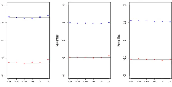
In order to verify the asymptotic behavior of Z(t), the test statistic of the K&K method with single t for testing geometric distribution described in Section 3.1.1, we calculate the empirical critical points of Z(t) for t =±0.01,±0.5,±0.9 (t is in the neighbor of zero or is not) based on 10,000 samples of size n = 50 from geometric distribution with p = 0.25 by Monte-Carlo simulations, and compare them with their theoretical counterparts from the standard normal distribution (see Figure 4.1).
Percentiles 99.5th and 0.5th percentiles −.9 −.5 −.01 .01 .5 .9 −4 −2 0 2 4 Percentiles 97.5th and 2.5th percentiles −.9 −.5 −.01 .01 .5 .9 −4 −2 0 2 4 Percentiles 95th and 5th percentiles −.9 −.5 −.01 .01 .5 .9 −3 −1.5 0 1.5 3
Figure 4.1 Empirical percentiles of Z(t) which is on the x-axis indicated by t value with n = 50 andp = 0.25.
Figure 4.1 shows that whentis closer to zero, the empirical critical points are closer to the corresponding standard normal percentiles. The empirical critical points are closer to the corresponding standard normal percentiles at the significance level α = 0.05 and 0.10 than atα = 0.01. Despite the difference in performance at different t0s and different significance
17
levels, overall the empirical critical points are satisfactorily close to the corresponding theoretical ones.
Similarly, in order to verify the asymptotic behavior of Tq(t), the test statistic of the
K&K method with multiplet’s for testing geometric distribution described in Section 3.1.2, we compute the empirical critical points ofTq(t) by simulations based on 10,000 replications
with n = 50 and p = 0.25, and compare them with their theoretical counterparts from the Chi-square distributions (see Table 4.1). Here in different cases, the number of t’s, q is chosen to be variate, i.e. q = 3, 5 or 10, and the values of t are chosen to be either in the neighborhood of zero or well spanned in interval (-1,1).
Table 4.1 Empirical Critical Points of Tq(t) based on 10,000 Replications
Statistics α = 0.01 α = 0.05 α = 0.1 T3(−0.15,−0.05,0.05) 11.349 7.672 6.113 T3(−0.90,0.05,0.85) 11.483 7.606 6.061 χ2 3 11.345 7.815 6.251 T5(−0.25,−0.15,−0.05,0.15,0.25) 14.647 10.759 9.018 T5(−0.90,−0.55,−0.15,0.25,0.90) 15.622 11.039 9.184 χ2 5 15.080 11.070 9.236 T10(−0.90,−0.75,−0.55,−0.35,−0.15,0.2,0.4,0.6,0.8,0.95) 25.547 17.580 14.971 χ2 10 23.209 18.307 15.987
In our calculation, we find that sometimes the entries of ˆΓ, see (3.4), are too small, which causes ˆΓ to be computationally singular. A threshold number of q exist for different type oft’s to avoid this problem. The threshold is larger when thetvalues spread well in the whole interval (-1,1) than when the t values are close to 0. Also computationally singular arises more often whenq = 10 than whenq = 3 and q= 5. Table 4.1 shows that overall the empirical critical points perform well in terms of being close to their respective Chi-square
percentiles. However, the empirical critical points are closer to the corresponding Chi-square percentiles whenq = 3 and q = 5 than when q = 10.
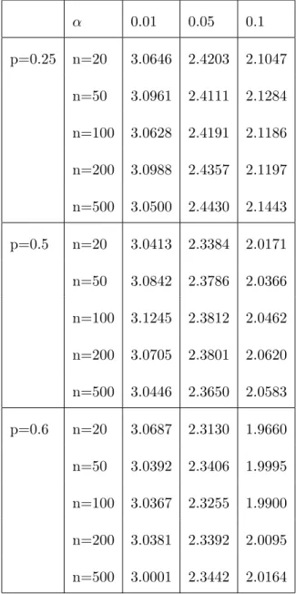
Now in order to explore the asymptotic distributions of SDn, the supremum test
statistic for testing geometric distribution described in Section 3.1.3, we calculate the empirical critical points of SDn for various p and n by parametric bootstrap with 10,000 bootstrap
samples, see Table 4.2 and plot the corresponding density curves (see Figure 4.2). Note that p= 0.25, 0.5 and 0.6, which are chosen corresponding to over dispersive, equally dispersive and under dispersive geometric distributions and thatn = 20, 50, 100, 200, 500 so that the asymptotic behavior of the critical points ofSDn can be studied.
0 1 2 3 4 5 6 7 0.0 0.1 0.2 0.3 0.4 0.5 0.6 For p = 0.25 SDn Density n=20 n=50 n=100 n=200 n=500 0 1 2 3 4 5 6 0.0 0.1 0.2 0.3 0.4 0.5 0.6 0.7 For p = 0.5 SDn Density n=20 n=50 n=100 n=200 n=500 0 2 4 6 8 0.0 0.2 0.4 0.6 0.8 For p = 0.6 SDn Density n=20 n=50 n=100 n=200 n=500
Figure 4.2 Density curves of SDn with variousp and n.
From Figure 4.2, we observe that for each pas n increases, the density curves of SDn
approach more and more close to each other, indicating a trend of achieving the limiting distributions. The curves attain a limiting density lot sooner for p = 0.25 case than for p = 0.5 and p = 0.6 cases. Table 4.2 indicates that the critical points ofSDn becomes fairly
19
Table 4.2 Empirical Critical Points of SDn based on 10,000 Bootstrap Samples
α 0.01 0.05 0.1 p=0.25 n=20 3.0646 2.4203 2.1047 n=50 3.0961 2.4111 2.1284 n=100 3.0628 2.4191 2.1186 n=200 3.0988 2.4357 2.1197 n=500 3.0500 2.4430 2.1443 p=0.5 n=20 3.0413 2.3384 2.0171 n=50 3.0842 2.3786 2.0366 n=100 3.1245 2.3812 2.0462 n=200 3.0705 2.3801 2.0620 n=500 3.0446 2.3650 2.0583 p=0.6 n=20 3.0687 2.3130 1.9660 n=50 3.0392 2.3406 1.9995 n=100 3.0367 2.3255 1.9900 n=200 3.0381 2.3392 2.0095 n=500 3.0001 2.3442 2.0164
4.2 Evaluating Tests by Comparison
Best and Rayner (2003) recommended A-D test for testing geometric distributions withp= 0.25, 0.5 or 0.6. Here we propose to compare Type I Errors and powers of the above tests with those of A-D, K-S and Chi-square tests under the same goodness of fit tests with the null hypothesis distribution specified as geometric distribution. Note that the value of geometric distribution in this comparative study starts from one not zero. We generate 10,000 Monte Carlo simulation replications of size n = 50 from the alternative distributions with the first moment equal to the one of the null distribution. The power is the proportion of replications
whose corresponding test statistic values greater than the 95th percentile indicating the null
hypothesis being rejected. Table 4.5, Table 4.6 and Table 4.7 show the power of various goodness-of-fit tests for geometric distributions withp = 0.25, 0.5 and 0.6, respectively.
In the Chernoff and Lehmann Chi-square test with test statistic χ2
cl1, the data is categorized into four groups: [1, 2], [3, 4], [5, 6], [7,∞). Soχ2
cl1 is asymptotically Chi-square distributed with two degrees of freedom when the null hypothesis is true. Similarly, in the other two Chernoff and Lehmann Chi-square tests with test statistics χ2
cl2 and χ2cl3, we categorize the data into three groups: [1], [2], [3, ∞). So the degree of freedom of the asymptotic distribution of χ2
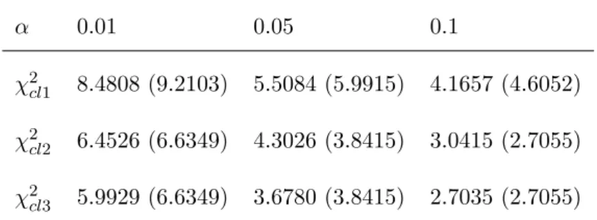
cl2 or χ2cl3, which is Chi-square distribution, is 1 when the null hypothesis is true. The empirical critical points of the Chernoff and Lehmann Chi-square test statistics are significantly deviating from their corresponding theoretical counterparts (see Table 4.3 in details). In order to have an accurate evaluation of the tests, we compare the goodness-of-fit tests based on their empirical critical points forχ2
cl1,χ2cl2 and χ2cl3.
Table 4.3 Empirical (Theoretical) Critical Points of χ2
cl1, χ2cl2 and χ2cl3 based on 10,000 Replications α 0.01 0.05 0.1 χ2 cl1 8.4808 (9.2103) 5.5084 (5.9915) 4.1657 (4.6052) χ2 cl2 6.4526 (6.6349) 4.3026 (3.8415) 3.0415 (2.7055) χ2 cl3 5.9929 (6.6349) 3.6780 (3.8415) 2.7035 (2.7055)
We apply the methods described in Best and Rayner (2003) to calculate the values of test statistics denoted byKS and AD for K-S and A-D tests, respectively. By Monte-Carlo simulations, we calculate their empirical critical points at α = 0.01, 0.05, 0.10 for n = 50 based on 10,000 replications. Table 4.4 shows the results. These critical points are used to compute powers and empiricalα in Table 4.5, Table 4.6 and Table 4.7.
We choose the following six types of alternative distributions as used in Best and Rayner (2003) for our comparative study. (1) BB(n, α, β): a beta binomial(BB) distribution with parameter n, α and β, where n is the number of trials, andα and β are parameters from a standard beta distribution; (2)NB(n, p): a negative binomial(NB) used to fit the number of
21
Table 4.4 Empirical Critical Points of KS and ADwith n= 50 based on 10,000 Replications
KS AD
p α=0.01 α=0.05 α=0.1 α=0.01 α=0.05 α=0.1
0.25 7.4840 6.1018 5.4259 1.9545 1.3118 1.0460
0.5 6.4421 4.9615 4.2494 2.0482 1.2771 0.9740
0.6 5.8806 4.4118 3.6842 1.8466 1.1429 0.8846
trials beforensuccesses with probability of successpfor each trial; (3)NA(λ1, λ2): a Neyman Type A (NA) distribution with probability mass function e−λ1λ
2/x!
P∞
i=0(λ1e−λ2)iix/i!, for x = 0,1,2, ...; (4) DU(i, j): a discrete uniform (DU) distribution with probability mess on i, i+ 1, ..., j; (5) B(n, p): a standard binomial distribution with n trials and probability of success p; (6) P M(ω1, ω2, λ1, λ2): a Poisson mixture(PM) where λi is a standard Poisson
distribution parameter for i = 1,2, and ω1 and ω2 are weights obtained between zero and one, which add up to one.
We use the standard functions inR 2.14 to generate geometric, binomial and negative binomial distributed random numbers, and the function rbetabinom.ab in package V GAM of R 2.14 to generate beta binomial distributed random numbers. Discrete uniformly distributed random numbers are obtained by inversing the cumulative distribution function. A Bernoulli distributed random value is created by using functionrbinominR2.14 with the number of trial one and probability of success ω1. If the value is one, we generate random numbers fromP(λ1) as the PM random numbers, otherwise from P(λ2), whereP(λi) is the
standard Poisson distribution with parameterλi for i= 1, 2. According to Best and Rayner
(2003), a random sample from the Neyman Type A distribution is generated as follows. First, generate a random sample (n1,n2, ...,ni) fromP(λ1). Then generateirandom samples from P(λ2), with size n1, n2, ..., and ni, respectively. Finally, sum up the data in each of the i
random samples fromP(λ2) to obtain a random sample of sizeifrom Neyman Type A. Since here the value of geometric distributed random variable starts from one not zero, the final
data from the alternative distributions are obtained by adding one to the generated random samples from the above six distributions.
In the case where the alternative distribution is NB(1, p), the power is equivalent to the significance level since NB(1, p) corresponds to geometric distribution with parameter p. See the highlighted rows in Table 4.5, Table 4.6 and Table 4.7.
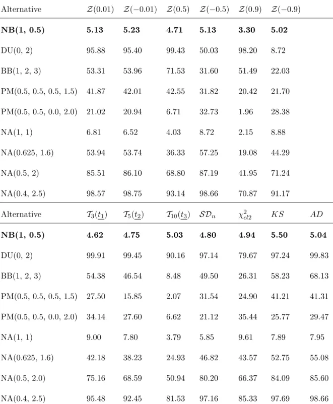
Table 4.5 Powers(%) for Geometric Tests withp = 0.25 atα= 0.05 based on 10,000 Samples of Sizen = 50 and the Mean of the Alternative is 4
Alternative Z(0.01) Z(−0.01) Z(0.5) Z(−0.5) Z(0.9) Z(−0.9) NB(1, 0.25) 5.05 4.97 4.87 4.82 3.76 4.70 BB(9, 1, 2) 23.97 22.78 52.95 10.16 63.68 7.21 BB(9, 0.5, 1) 7.66 7.42 3.05 8.53 7.18 5.41 NA(1, 3) 71.45 71.68 33.51 79.80 4.32 52.58 NA(0.95, 3.16) 79.86 80.97 43.91 87.17 7.02 60.17 NA(0.9, 3.33) 88.08 89.10 55.32 92.84 9.50 69.04 Alternative T3(t1) T5(t2) T10(t3) SDn χ2cl1 KS AD NB(1, 0.25) 5.01 5.13 3.90 5.12 4.94 4.98 5.15 BB(9, 1, 2) 38.05 42.24 28.47 41.23 32.85 47.68 60.33 BB(9, 0.5, 1) 8.97 24.34 27.16 6.63 12.03 18.84 23.62 NA(1, 3) 74.80 66.87 45.69 67.51 12.82 65.07 67.62 NA(0.95, 3.16) 83.02 76.93 56.27 78.95 13.59 73.67 77.67 NA(0.9, 3.33) 89.81 84.96 66.89 86.10 15.73 83.03 84.81 wheret1= (-0.15, -0.05, 0.05),t2= (-0.25, -0.15, -0.05, 0.15, 0.25),t3= (-0.9, -0.75, -0.55, -0.35, -0.15, 0.2, 0.4, 0.6, 0.8, 0.95).
In Table 4.5, Z(0.01), Z(−0.01) Z(−0.5), T3(t1), SDn have higher powers than KS
and AD for NA alternatives while they all maintain Type I error probability close to 5%. However,AD performs the best overall for BB alternatives. Theχ2
cl1 performs the worst for NA alternatives and moderately for BB alternatives. Obviously, the choice of goodness-of-fit
23
Table 4.6 Powers(%) for Geometric Tests with p = 0.5 at α = 0.05 based on 10,000 Samples of Sizen = 50 and the Mean of the Alternative is 2
Alternative Z(0.01) Z(−0.01) Z(0.5) Z(−0.5) Z(0.9) Z(−0.9) NB(1, 0.5) 5.13 5.23 4.71 5.13 3.30 5.02 DU(0, 2) 95.88 95.40 99.43 50.03 98.20 8.72 BB(1, 2, 3) 53.31 53.96 71.53 31.60 51.49 22.03 PM(0.5, 0.5, 0.5, 1.5) 41.87 42.01 42.55 31.82 20.42 21.70 PM(0.5, 0.5, 0.0, 2.0) 21.02 20.94 6.71 32.73 1.96 28.38 NA(1, 1) 6.81 6.52 4.03 8.72 2.15 8.88 NA(0.625, 1.6) 53.94 53.74 36.33 57.25 19.08 44.29 NA(0.5, 2) 85.51 86.10 68.80 87.19 41.95 71.24 NA(0.4, 2.5) 98.57 98.75 93.14 98.66 70.87 91.17 Alternative T3(t1) T5(t2) T10(t3) SDn χ2cl2 KS AD NB(1, 0.5) 4.62 4.75 5.03 4.80 4.94 5.50 5.04 DU(0, 2) 99.91 99.45 90.16 97.14 79.67 97.24 99.83 BB(1, 2, 3) 54.38 46.54 8.48 49.50 26.31 58.23 68.13 PM(0.5, 0.5, 0.5, 1.5) 27.50 15.85 2.07 31.54 24.90 41.21 41.31 PM(0.5, 0.5, 0.0, 2.0) 34.14 27.60 6.62 21.12 35.44 25.77 29.47 NA(1, 1) 9.00 7.80 3.79 5.85 9.61 7.89 7.95 NA(0.625, 1.6) 42.18 38.23 24.93 46.82 43.57 52.75 55.08 NA(0.5, 2.0) 75.16 68.59 50.94 80.20 66.37 84.09 85.60 NA(0.4, 2.5) 95.48 92.45 81.53 97.16 85.33 97.69 98.66 wheret1= (-0.15, -0.05, 0.05),t2= (-0.25, -0.15, -0.05, 0.15, 0.25),t3= (-0.9, -0.75, -0.55, -0.35, -0.15, 0.2, 0.4, 0.6, 0.8, 0.95).
tests in this context would depend upon what the alternative distribution is for a given problem.