I. Using R for Statistical Tables and Plotting Distributions
TheRsuite of programs provides a simple way for statistical tables of just about any probability distribution of interest and also allows for easy plotting of the form of these distributions. In what follows below, R commands are set inbold courier. Note thatRcommands are CASE-SENSITIVE, so be careful when typ-ing.
General Syntax for Distribution Functions
There are four basicRcommands that apply to the various distributions defined in R. LettingDISTdenote the particular distribution andparametersthe parameters to specify that distribution (see Table one), the basic syntax of the four basic commands are:
dDIST(x, parameters)— probability density of DIST evaluated atx. qDIST(p, parameters)— returnsxsatisfying Pr(DIST(parameters)≤x) =p pDIST(x, parameters)— returns Pr(DIST(parameters)≤x)
rDIST(n, parameters)– generatesnrandom variables from DIST(parameters)
Table 1. Common continuous probability distributions inR. If certain parameters are not specified, the default is assumed. For example, a unit normal unless the mean and variance are specified, and a central distribution unless a noncentrality parameter is given. Other continuous distributions are given in Table 2 (below).
Distribution Syntax
Normal norm()— unit normal (the default) norm(µ, σ2)
— normal with meanµand varianceσ2
.
Student’s t t(df)— centraltwithdfdegrees of freedom (default) t(df,ncp)— noncentraltwith noncentrality parameterncp
χ2 chisq(df)
– centralχ2
withdfdegrees of freedom (default) chisq(df,ncp)– noncentralχ2with noncenturality parameterncp F f(df1,df2)– centralFwithdf1anddf2degrees of freedom (default)
f(df1,df2,ncp)— noncentralFwith noncenturality parameterncp
Plotting Probability Distributions
One very powerful feature ofRis its ability to quickly plot any number of functions for the desired distribution. The command used for plotting is thecurvefunction: •curve(function,xlow,xhigh)– plotsfunctionbetween xlow and xhigh
•curve(function,xlow,xhigh,n=500) – plots function using 500 equally-spaced points
Example 1: Suppose we wish to plot a (central)χ2distribution with 5 degrees of freedom, say between 0 and 30. To do this inRtype the following:
curve(dchisq(x, 5), 0, 30) typing
curve(dchisq(x, 5), 0, 30, n = 500) uses 500 (equally spaced) points to draw the curve
Suppose that we now wish to examine the effect of moving from a centralχ2
distribution to an increasingly noncentralχ2
. The distribution function for the noncentralχ2distribution inRis given bydchisq(x, df,ncp), wheredf are the degrees of freedom andncpthe noncentrality parameter. To add an ad-ditional curve to the one plotted, we use theadd=TRUEcommand in thecurve function. For example, to add a curve for eχ2
with noncentrality parameter 10, curve(dchisq(x, 5,10), 0, 30,add=TRUE)
Ralso lets you specify the color, by using thecol = "COLOR"command, for example
curve(dchisq(x, 5,10), 0, 30,add=TRUE,col="pink") adds this curve in pink (Rhas a wide range of colors, so have fun).
Example 2: Rcan also be used to plot cumulative probability densities. For example,
curve(dt(x, 5), 0, 30)
plots the cumulative probabilities for a student’stwith 5 degrees of freedom forxranging from -3 to +3.
curve(pt(x,5,1), -3, 3, add=TRUE, col="green")
overlays a green curve for cumulative probability for a noncentraltwith non-centrality parameter 1.
We can also point the requiredxvalues for a givenpvalue. For example, for a (central) F distribution with 2 and 20 degrees of freedom, since nowx(the probability) ranges from zero to one,
curve( qf(x,2,20), 0, 1)
Obtainingp and Critical Values
ThepDIST(x, parameters) returns thepvalue associated with a particularx value drawn from that distribution, i.e., returns Pr(DIST(parameters)≤x). Con-versely, theqDIST(p, parameters) returns the xvalue to give a particular p value.
Example 3: . What is thexvalue from a student’stdistribution with 12 degrees of freedom so that there is a 99 % probability that a random value is belowx? Typing
qt(0.99,12) inRreturns2.680998.
Likewise, if we have a noncentralt (with noncentrality parameter 1.75) and observe a value of 3.5, the probability of being this value or less is given by
pt(3.5,12,1.75)
or0.91566. Thepvalue is one minus this (as Pr(DIST> x) = 1-Pr(DIST≤x), or
1- pt(3.5,12,1.75) which equals0.08433496.
Example 4: Two-side confidence α-level confidence intervals are given by xmin, xmax, where Pr(DIST≤(xmin) = (1−α/2)and Pr(DIST≤(xmax) = 1−(1−α/2). For example, an 99.9% confidence interval for a unit normal hasα= 0.999, and hence(1−α)/2 = 0.0005. We can obtain upper and low values inRby typing
qnorm( 0.0005 ) and
As an example of using other features ofR, we can also compute these by first specifying toRtheαvalue we wish to use by typing
alpha <- 0.999
This tellsRthat we have assigned alpha the value of 0.999. The lower and upper (respectively) values follow from
qnorm((1-alpha)/2) and
qnorm( 1-1-alpha)/2 Ragain returns values of-3.290527, 3.290527.
Another usefulRis that we can input a vector of values and for many of the distribution commandRwill output a vector of the designed values. We can define the vector of the upper and lower probabilities (for which we desire associated critical values) by
xvals <- c((1-alpha)/2, 1-(1-alpha)/2)
Here the commandc()means create a vector from the (in this case two ) items in the list, and assign the variablexvalsthe value of this vector. Typing in
qnorm( xvals ) Ragain returns-3.290527 3.290527.
Example 4: While confidence intervals for normal and studenttvariables are symmetric, those for χ2
andF distributions are not. For example, the 95% confidence interval for anFdrawn from a distribution with 2 and 20 degrees of freedom is (lower value)
alpha <- 0.95 qf((1-alpha)/2,2,20) or0.02534988and an upper value of
qf(1-(1-alpha)/2,2,20) for4.461255.
Other Continuous Probability Distributions
Table 2. Some other continuous probability distributions inR. If certain parameters are not specified, the default is assumed. For exact details of how the parameters are defined, see theRhelp file. Note that this is not a complete set, so check the help file if a distribution is not listed here, asRlikely has it.
Distribution Syntax
Exponential exp()— Exponential with rate 1 (the default) exp(rate)— Exponential with rate set by user
Uniform unif()— Uniform on (0,1) (the default) unif(min, max)— Uniform over (min, max)
Log Normal lnorm()—log normal with meanlog=0, SD of log = 1 (the default) lnorm(meanlog,sdlog)—log normal with meanlog, SDlog
Beta beta(shape1, shape2)—beta with shape parameters shape1, shape 2
Gamma gamma(shape)—gamma with shape user specified, scale=1. (the default) gamma(shape,scale)— scale parameter set by user.
Weibull weibull(shape)—Weibull with shape user specified, scale=1. (the default) weibull(shape,scale)— scale parameter set by user.
Wilcox wilcox(m,n)—Distribution for Wilcoxon rank sum statistic with sample sizes m and n.
Discrete Probability Distributions
Table 3 lists several of the discrete probability distributions avilable inR.
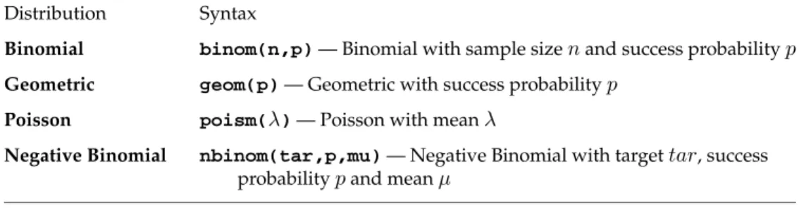
Table 3. Some of the discrete probability distributions inR. Distribution Syntax
Binomial binom(n,p)— Binomial with sample sizenand success probabilityp
Geometric geom(p)— Geometric with success probabilityp
Poisson poism(λ)— Poisson with meanλ
Negative Binomial nbinom(tar,p,mu)— Negative Binomial with targettar, success probabilitypand meanµ
Example 5. In order to plot a discrete function, we must first generate a se-quence of integers.Rcan be used to generate a sequence as follows:
x <- seq(0,25,1)
this generates a seqeunce from 0 to 25 in steps of one and then stores the resulting sequence in the variable x. More generaly to generate a sequence from a to b in steps of c, we would useseq(a,b,c).
To plot the first 26 values (for 0 to 25) for a Poisson distribution with parameter λ= 3, inRusing the above sequence, now type:
plot(dpois(x,3))
Adding thetype =""command can change the points into a step latter graph (type = "s") or a histogram (type ="h"), so that
plot(dpois(x,3),type="s") plots a step latter function while
plot(dpois(x,3),type="h") plots a histogram.
You will notice that the plot values are essentially zero from values greater than 10. If we wish more discrimation, we can plot the log of the probabilities. This is done in thedDISTcommand by using the optionlog=TRUE, which returns the log of the probabilities (log=FALSEis the default which is used unless otherwise specificed by the user). Hence, to plot the log of probabilities (as a histogram) for the 51 terms in a Binominal withn= 50and success probability p= 0.8, type x <- seq(0,50,1) then plot(dbinom(x,50,0.8,log=TRUE),type="h") while plot(dbinom(x,50,0.8),type="h") plots the probabilities on a linear scale.