Espoo 2005 TKK-INIT-2
BUSINESS PROCESS MODELING AND SIMULATION
Espoo 2005 TKK-INIT-2
BUSINESS PROCESS MODELING AND SIMULATION
Alexander Sidnev, Juha Tuominen, Boris Krassi
Helsinki University of Technology
Department of Computer Science and Engineering Industrial Information Technology Laboratory
Industrial Information Technology Laboratory P.O. Box 5400 TKK FIN-02015 Espoo Finland Fax: +358-9-451-5351 www.init.hut.fi
© Alexander Sidnev, Juha Tuominen, Boris Krassi
ISBN: 951-22-7928-2 (printed version) ISBN: 951-22-7929-0 (electronic version) ISSN: 1459-6458
Otamedia Oy Espoo 2005
Department/laboratory and URL/Internet address
Computer Science and Engineering
Industrial Information Technology Laboratory www.init.hut.fi
Publisher
Otamedia Oy
Authors
Alexander Sidnev, Juha Tuominen, Boris Krassi
Title
Business Process Modeling and Simulation
Abstract
The textbook provides the essentials of the Business Process (BP) Modeling and Simulation (M&S) from the verbal BP description to the formulation of the mathematical scheme of the model and the simulation program.
Both the analytical modeling and the simulation approaches to BP M&S are considered. Special attention is given to the theoretical and practical aspects of the ВР M&S. The text covers the following topics: fundamentals of the BP M&S, conceptual modeling using IDEF3 standard, cost metrics and the activity based costing, analytical modeling (queuing networks, linear and dynamic programming), simulation with GPSS, timed Petri Nets, and Crystal Ball toolkits. Case studies include BP simulations with BPwin and GPSS.
The intended readers are senior graduate students and junior postgraduate students of computer science and industrial management.
Keywords
BP modeling and simulation, linear programming, dynamic programming, timed Petri nets, queuing networks, activity based costing, GPSS
Place Espoo Year 2005 Number of pages 116 Language of publication English Language of abstract English ISBN (printed) 951-22-7928-2 ISSN (printed) 1459-6458 ISBN (electronic) 951-22-7929-0
URL (Internet address)
LIST OF ABBREVIATIONS
ABC Activity-based costing
BP Business process
BPwin BP simulation software of Computers Associates International, Inc
CEC Current event chain
FEC Future event chain
GPSS General purpose simulation system
IDEF Integrated family of integration definition methods
IDEF0 Integration definition for function modeling
IDEF3 Integration definition (IDEF) method for process description capture
M&S Modeling and simulation
OROS Trademark of ABC Technologies
CONTENTS
LIST OF ABBREVIATIONS ...4
CONTENTS ...5
AKNOWLEDGEMENT ...8
PREFACE...9
CHAPTER 1. MODELING AND SIMULATION AS THE BUSINESS PROCESS REENGINEERING TOOL ...10
1.1. Business process reengineering as a subject of system analysis...10
1.2. Applying operations research to the business process reengineering ...11
CHAPTER 2. INTRODUCTION TO MODELING AND SIMULATION...13
2.1. Analytical modeling vs. simulation...13
2.2. Types of models ...13
2.3. Structure of the simulation process ...14
CHAPTER 3. USING IDEF FORMAT FOR THE BP MAPPING...17
3.1. Function modeling (IDEF0)...17
3.2. Process modeling (IDEF3)...18
CHAPTER 4. ACTIVITY-BASED COSTING AS BP COST METRICS...21
4.1. АВС as an approach to the true costs analysis...21
4.2. Steps of ABC...23
4.3. Comparison of the cost models ...25
4.4. ABC toolkits...26
CHAPTER 5. ANALYTICAL BP MODELING...28
5.1. Steps of the analytical modeling ...28
5.2. Classification of the BP models ...29
5.3. Deterministic BP models DRDT&C ...30
5.3.1. Bellman’s dynamic programming for the BP scheduling...33
5.3.2. BP scheduling as a problem of mathematical programming ...36
5.3.3. BP resource optimization by means of mathematical programming...40
5.4. Stochastic BP models: DRPT&C and PRPT&C ...43
5.4.1. DRPT&C model ...43
5.4.1.1. BP scheduling analysis with Crystal Ball...45
5.4.2. Stochastic PRPT&C models with an account for the resource utilization...49
5.4.2.2. Representing the BP IDEF3 model as the queuing network... 53
CHAPTER 6. BP SIMULATION WITH GPSS... 59
6.1. GPSS fundamentals ... 59
6.1.1. System representation... 59
6.1.2. GPSS language... 59
6.2. BP IDEF3 model interpretation for the GPSS modeling... 63
CHAPTER 7. OUTPUT ANALYSIS... 66
7.1. Precision of the simulation results... 66
7.1.1. Point estimation... 66
7.1.2. Interval estimation... 66
7.1.3. Estimating the confidence interval... 67
7.2. Selecting the sample size... 68
CHAPTER 8. BP SIMULATION WITH THE TIMED PETRI NETS... 69
8.1. Petri nets ... 69
8.2. BP modeling with the F-Net toolkit... 70
8.3. Examples of the timed Petri nets for the BP modeling... 71
8.3.1. Example 1: unlimited resources ... 71
8.3.2. Example 2: taking the resources limitation into account ... 74
CHAPTER 9. CASE STUDY OF THE BP MODELING WITH GPSS... 79
9.1. Problem definition ... 79
9.1.1. BP IDEF3 model ... 80
9.1.2. Activity definition ... 90
9.2. Activity costing... 90
9.2.1. Assigning activities to executors. Activity cost data... 90
9.3. GPSS BP model parameters ... 92 9.3.1. Input parameters ... 92 9.3.2. Output parameters ... 92 9.4. BP research using GPSS... 93 9.4.1. GPSS open model... 93 9.4.2. GPSS closed model ... 93 9.4.3. Preventing deadlocks... 95 9.4.4. BP research... 95
CHAPTER 10. SAMPLE BP M&S TRAINING TASK ... 98
10.2. Defining the BP cost model ...98
10.3. Creating the BP analytical models ...98
10.3.1. Bellman’s dynamic programming for the BP scheduling...99
10.3.2. Mathematical programming for the BP scheduling...99
10.3.3. BP probabilistic analysis...99
10.3.4. Queueing networks for the BP analysis...100
10.4. Creating the GPSS BP model...100
10.5. Creating the ABC model of the BP...100
10.6. Creating the BP model in the form of the timed Petri nets ...100
10.7. Drawing conclusions...100
REFERENCES ...101
GLOSSARY OF THE KEY TERMS...102
INDEX...103
APPENDIX A. GPSS PROGRAMS FOR MODELING EXAMPLE BUSINESS PROCESSES ...106
APPENDIX B. GPSS PROGRAM FOR MODELING THE ENTERPRISE CONSULTING RESEARCH ...112
AKNOWLEDGEMENT
The textbook is based on the lecture notes of the “Business Process Modeling and Simulation” course, which was delivered by Dr. Sidnev at Helsinki University of Technology in May 2004 and September-October 2005. The guest lectures of Dr. Sidnev have been supported by the Academy of Finland.
PREFACE
Paraphrasing Robert Shannon [15], the business process (BP) modeling and simulation (M&S) is probably as much art as science. The subject of this textbook concerns the science of ВР M&S, in other words, the part of the BP M&S that can be formalized.
The textbook is based on the lecture notes of “Business Process Modeling and Simulation” course, which was delivered in May 2004 and September-October 2005 for postgraduate students at Helsinki University of Technology.
The basic idea of the book is to consider the capabilities of M&S applied to the BP analysis and synthesis. Equal attention is paid to the following complementary approaches – the ВР analytical modeling vs. the ВР simulation – as it is expedient to use both of them together. While the analytical models allow formalizing the complicated problems of the ВР
synthesis, the BP simulation insures an acceptable accuracy of the ВР analysis.
The mathematical basis of the material given in the textbook includes systems analysis, probability theory, and theory of queuing networks. Some knowledge of these mathematical disciplines is desirable, but not necessary since the basic introduction is given whenever needed.
The theory is illustrated with a comprehensive example used throughout the text. The text contains 10 chapters.
Chapters 1 and 2 contain the definitions of the basic ideas of system analysis, which are relevant to the ВР M&S.
Chapter 3 is devoted to the basics of the IDEF3 standard employed as a construction tool of the ВР conceptual modeling.
Chapter 4 explains the fundamentals of ABC as the basis of the ВР cost metrics. Chapter 5 offers the methods of the ВР analytical modeling based on dynamic and linear programming, and theory of queuing networks.
Chapters 6 through 9 are dedicated to the topic of the BP simulation.
Chapters 6 and 9 contain the basics of the ВР simulation using GPSS and a case study of the BP GPSS model development.
Chapter 7 describes the process of estimating the accuracy of the BP simulation exploiting the methods of mathematical statistics.
Chapter 8 describes the approach to the BP simulation with the timed Petri nets. Chapter 10 contains a sample BP M&S training task.
CHAPTER 1. MODELING AND SIMULATION AS THE BUSINESS PROCESS REENGINEERING TOOL
“Business process reengineering (BPR) is the fundamental rethinking and radical redesign of business processes to achieve dramatic improvements in critical, contemporary measures of performance, such as cost, quality, service and speed” [1].
The following four key words are to be outlined in this definition:
• Fundamental means starting from scratch in the business organization rethinking;
• Radical implies demolishing the company structure rather than marginally
improving it;
• Process indicates focusing on the process rather then the structure. This concept
requires a detailed investigation of the process-oriented mapping of activities;
• Measures of performance mean the estimating of the system’s quantitative and
qualitative characteristics.
To achieve the desired significant improvements on the way of the radical business processes redesign, it is important to insure that there are no mistakes and those radical changes would indeed lead to the expected results.
BPR is a very costly affair. Therefore, assessing the profit of the BPR efforts is crucial to decide whether to undertake the BPR. The BP M&S is often the only way to answer this question.
1.1. Business process reengineering as a subject of system analysis
Systems Analysis is a scientific domain of the semi-structured complex interdisciplinary problem research. Systems Analysis is based on the following four fundamental principles:
• System approach to the subject research;
• Hierarchy, i.e. the multilevel research of the subject;
• Synergy principle, which is based on the idea that a system is greater than a mere
sum of its elements;
• Formalism means that the subject is represented as a formal model, which makes
it possible to achieve constructive results.
The subject of Decision Taking is one of the essential tasks of Systems Analysis, while Operations Research is a discipline providing the proof of the taken decision.
1.2. Applying operations research to the business process reengineering
Definitions
Operation is a collection of mutually agreed actions directed at achieving a defined goal.
Operation solution is a collection of parameters, which define the way of how the operation is executed.
Unguided operation factors are real probabilistic conditions that affect the outcome of the operation.
Operation Efficiency or Objective Function is a quantitative estimate of the operation outcome.
Problems of the Operations Research
Operations Research Model creation. Mathematical Operation Research Model is defined as follows:
(
x X z Z)
z x f( , ), ∈ ; ∈ , (1.1) where: ) , (x z f is an objective function; x is an operation solution;X is a set of admissible solutions; z are unguided operation factors; Z is a set of unguided factors.
Analysis of the Operation means estimating the selected solution, i.e. finding the value of the objective function f(x,z) for the solution . x
Synthesis of the Operation means finding the optimal solution, which maximizes (minimizes) the objective function:
. , ) , ( max(min) Z z X x z x f x ∈ ∈ →
Business process reengineering as the BP modeling problem
With the reference to the BPR, the Operations Research Model creation can be formulated as determining the dependence of the objective function on the business process parameters.
Selecting the objective function is left beyond the scope of the book. The objective function may be, for example, a temporal or cost BP parameter or an integral criterion in the form of a weighted sum of some local criteria.
If it is possible to construct BP analytical model, i.e. to find an explicit function of the BP organization parameters, the problem of the BP optimization turns out to be a problem of mathematical programming.
) , (x z f
If it is impossible to create a BP analytical model, the problem of determining can be solved by means of simulation in conjunction with the statistical testing.
) , (x z f
To sum up, the BP mathematical model creation is a necessary stage of its research. Some examples of defining the BP analysis problems in terms of the operations research are presented in Sec. 5.3.1 and 5.3.2.
CHAPTER 2. INTRODUCTION TO MODELING AND SIMULATION
A thorough introduction to the system simulation with a number of examples can be found in [2].
Simulation is an imitation of a real-world process or system over a period of time. Simulation involves creating a simulation model of the real system, generating an artificial history of the system by substituting the system with the simulation model, and observing the artificial history to draw the inferences regarding the operation characteristics of the real system.
Sometimes it is possible to develop such a model, which is simple enough to be handled by the analytical methods. If this is the case, the model is called analytical.
Both analytical and simulation models are represented in the mathematical form (formulae, tables, plots, algorithms, logic expressions, etc.).
2.1. Analytical modeling vs. simulation
The analytical model enables to obtain the most general results on the behavior of the real system, which are usually represented in the form of strict mathematical expressions.
A disadvantage of the analytical modeling lies in its limited capabilities of adequately mapping real complex systems. The analytical model is bounded by its mathematical scheme.
The simulation model has a larger “mapping capacity” than the analytical model because it is easier to observe the behavior of a system than to get into its underlying principles of management and development.
In many cases simulation is the only way to start the development of a complex system.
A disadvantage of the simulation approach is the form of the modeling results. Each simulation run provides a point-to-point mapping for the sets of the input and the output variables. This disadvantage can be tackled by conducting multiple simulations.
2.2. Types of models
There are many ways of classifying system models. One possible way with five most relevant clustering criteria is shown in Fig. 2.1.
Types of models Discrete Continuous Mathematical Physical Static Dynamic Deterministic Stochastic Analytical Simulation Combined
Figure 2.1. Classification of models
• Discrete vs. continuous models (it often depends on the point of view rather than the nature of the modeled system);
• Mathematical vs. physical (material, not virtual);
• Static vs. dynamic;
• Deterministic vs. stochastic;
• Simulation vs. analytical (or combined).
2.3. Structure of the simulation process
The main steps of the simulation study are listed below in the order of their execution and interdependencies (see Fig. 2.2):
• Formulating the problem;
• Setting the objectives;
• Conceptualizing the model;
• Defining the initial data and the quantitative parameters of the model;
• Translating the model;
• Verifying and validating the model;
• Executing the simulation runs and analyzing the results;
Let us consider these steps in more detail.
Formulating the problem and setting the objectives
M&S is aimed at reflecting features of the system in question. There is no sense to start modeling without having the purpose of modeling in mind. So, at first the problem has to be formulated (questions, hypotheses).
It is essential to set the objectives of M&S, which are relevant and adequate to the problem at hand. The objectives may include costs, temporal parameters, reliability etc. Hardly is it possible to model the system unless the objectives are clearly defined.
Conceptualizing the model
The first stage of formalizing the model is to select the basic assumptions, which characterize the system results in the conceptual model creation. The conceptual model defines the system elements and the way of their interaction. It is the basis of the mathematical scheme to be implemented in the form of a simulation or an analytical model.
Translating the model
The model must be represented in a computer recognizable format. There are two competing ways of solving this problem: (1) building the model in some universal programming language and (2) using a dedicated simulation language. Each way has its pros and cons. On the one hand, the universal programming language approach is often easier, but it requires quite a good self-made simulation system for driving the simulation program. On the other hand, the dedicated simulation language gives the modelers all the abilities of a powerful simulation system, but it constrains them by the limits of the modeling concept.
Verifying and validating the model
Verification refers to the process of insuring that the model is free from logical errors, i.e. that the model does what it is intended to do.
Validation insures that the model is a reasonable and valid representation of the real system or problem.
Unlike validation, the task of verification is quite formal. Executing the simulation runs and analyzing the results
This step has two major aspects: (1) designing the simulation experiment to generate the output data, which would be sufficient for the subsequent system investigation, and (2) determining the number of observations required for achieving the desired precision of the simulation results. The second aspect will be considered in Ch. 7.
Model Verified ?
Sufficient number of runs?
Model Validated ?
Documenting and
Reporting
Formulating the Problem
Setting the Objectives
Collecting the Data
Conceptualizing the Model
Translating the Model
Executing Runs
Interpreting and Analyzing
the Results
Yes No Yes No Yes NoCHAPTER 3. USING IDEF FORMAT FOR THE BP MAPPING 3.1. Function modeling (IDEF0)
IDEF stands for the Integration Definition. It also refers to a family of mutually-supportive methods for enterprise integration.
IDEF0 is the Integration Definition for Function Modeling.
IDEF0 model is a graphical description of the system, which is developed for a
specific purpose and considered from a certain viewpoint.
Function is an activity identified by a verb or verb phrase that describes what must be
accomplished.
Box is a rectangle, which contains a name and a number. It represents a function.
Input Arrow is a class of arrows that expresses the IDEF0 input, i.e. the data or the
objects that are transformed by a function into the output.
Output Arrow is the class of arrows that expresses the IDEF0 output, i.e. the data or
the objects produced by a function.
Mechanism Arrow is a class of arrows that expresses the IDEF0 mechanism, i.e. the
means of performing a function.
Call Arrow is a type of the mechanism arrow that enables to share details between
models (linking models together) or within a model.
Control Arrow is a class of arrows that expresses the IDEF0 control, i.e. the
conditions required to produce the correct output.
Function modeling (IDEF0) uses activities and arrows to describe and to document the business processes, see Fig. 3.1. Creating a business process model starts from the context diagram with the only activity, which represents the model, see Fig. 3.2.
The context diagram depicts the highest-level activity in the model. It represents the boundary of the process with respect to the purpose, scope, and viewpoint. Subsequently, one can add the decomposition of the activities and the arrows to specify and to refine the business process model.
The IDEF0 standard uses several types of links between the activities. The arrows can change their type. For example, an Output arrow may become a Control arrow and vice versa. IDEF0 employs a multilevel decomposition of the activities in order to come to a set of elementary activities, which can be explicitly depicted. That is the way to create a coherent function description.
Figure 3.1. Function modeling (IDEF0)
Figure 3.2. Context diagram of a business process (screenshot: BPwin ®)
3.2. Process modeling (IDEF3)
Process Flow modeling, also referred to as IDEF3 modeling, is a modeling methodology used for graphical description and documentation of processes by capturing the
Activity
Control
Output Input
information on the process flow, the relationships between processes, and those important objects that are part of the process.
Unit of Behavior (UOB) is a term used in IDEF3 to describe types of events or “happenings”.
UOB Box (Unit of Work, UOW) is a syntactic element of the IDEF3 Schematic Language, which is employed to represent a real-world process. It is similar to the Activity term in the IDEF0 format.
Decomposition of a UOB is a method of tackling the process complexity.
Processes are represented on the schematic diagram as labeled boxes, see Fig. 3.3. Each box represents packets of information about an event, a decision, an act, or a process, i.e. the types of “happenings”.
The logic functions named “junctions”, which are included in the IDEF3 syntax, are aimed at defining the logic connection between the source and the target boxes.
The information about a UOB comprises:
1. Name (often verb-based) indicating what the UOB represents;
2. Names of the objects, which are included in the process, and their properties;
3. Relations between the objects. The arrows (called links) connecting the boxes indicate the precedence relationships (more generally, constraints) between the processes. Thus, the UOB instance at the source of a link completes prior to the start of the UOB instance at the end of the same link.
The BP mapping by means of the IDEF3 standard becomes a true conceptual BP model when it is filled with data (mostly quantitative) about all the details of each UOB.
CHAPTER 4. ACTIVITY-BASED COSTING AS BP COST METRICS
4.1. АВС as an approach to the true costs analysis
Activity-based Costing (ABC) is a management methodology developed in the 1980’s as a practical solution for some of the problems associated with the traditional cost management systems [3] 1. The problem of cost metrics is relevant to the BP modeling for the following two reasons. First, the cost metrics are important for estimating the BP efficiency. Second, since a simulation model is capable of performing only those actions that are determined in the form of strict algorithm, the algorithm should include the calculations of the cost metrics.
Companies may have significant overhead costs. Every company has to spend financial resources to maintain a number of its activities, which are not directly profitable, for instance, marketing, scientific research, consulting assistance and so on. An important problem of the traditional cost systems is their inaccuracy in assessing the overhead costs.
The activity-based cost systems extend traditional ones by linking the resource expenses to the variety and the complexity of products rather than only to the physical volumes of production. The ABC principles are explained in detail in [3], the book of the ABC founders.
To highlight the difference between ABC and the traditional methods, let us examine the structure of the traditional cost system (Fig. 4.1), where the factory overhead costs are allocated to the production cost centers. Allocating (not evaluating) the overhead costs is the key feature of the traditional cost systems. The traditional cost systems easily fail when allocating the overhead expenses of the cost centers (in proportion with the direct labor hours or the machine hours) to the production cost centers.
Sometimes the best of the traditional cost systems can be quite accurate if they directly assign the overhead costs to the production cost centers (based on the actual usage). However, even these systems fail at the next stage, when the costs, which are accumulated at the production cost centers, are assigned to the products processed at each center.
ALLOCATING OVERHEAD COSTS TO PRODUCT COST CENTERS AND THEN TO PRODUCTS
Center
1
Center
2
Center
k
ALLOCATIONS
PRODUCTION COST CENTERS PROD. COST CENTER 1 PROD. COST CENTER m PROD. COST CENTER g MACHINE HOURS
PRODUCT 1 PRODUCT g PRODUCT m
DIRECT MATERIALS DIRECT LABOR
OVERHEAD COST CENTERS
DIRECT LABOR HOURS
Figure 4.1. Structure of the traditional cost system (based on [3], p.83)
Fig. 4.2 shows the structure of an Activity-Based Cost system. At the first glance, the ABC system appears to be similar. Nevertheless, the underlying structure and the concept are quite different. The focus of the ABC is shifted from how to allocate the costs to why the organization spends the financial resources in the first place.
The development of the ABC systems comprises four steps [3], which are discussed in the next section.
RESOURCE EXPENSES
RESOURCE 1 RESOURCE 2 RESOURCE K
ACTIVITY 1 ACTIVITY M ACTIVITY 2 PRODUCT 1 PRODUCTR PRODUCTN DIRECT MATERIALS DIRECT LABOR
ABC Traces Resource Expenses to Activities
ACTIVITY COST DRIVERS RESOURCE COST DRIVERS
Figure 4.2. Structure of the ABC system (based on [3], p. 84)
4.2. Steps of ABC
Step 1. Develop the activity dictionary
First of all, the organization has to identify the activities associated with its indirect and support expenses.
The activity dictionary is a list of the activities employed within the organization. An entry of the list contains the name of an activity, its definition, output, and appropriate classification.
activities, especially if the prime focus of the ABC system is on estimating the product and the customer costs. The activities that consume less than 5% of the resource capacity are usually not included in the dictionary. However, there exist ABC systems with hundreds of activities.
Step 2. Determine how much the organization spends for each of its activities
The ABC system maps the resource expenses to the activities by means of the resource cost drivers. The resource cost drivers link the spending and the expenses, as captured in the general accounting system, to the performed activities. Business process cost structure should comply with its IDEF-model. The actual mechanics of selecting the resource cost drivers and estimating the quantity of each resource cost driver have to be reasonably well described in the model. BPwin Cost Editor2 can be employed at the step.
Step 3. Identify the organization’s products, services, and customers (cost objects)
Step 3 is simple but important. The question of whether one or another activity or process is worth doing is not trivial. Answering the question requires the activity costs being linked to the products, services, and customers.
Step 4. Select the activity cost drivers, which link the activity costs to the organization’s products, services, and customers
A cost object is a product, a service, a customer, a location, a unit, a project or a work objective, for which an individual cost measurement is needed.
The linkage between the activities and the cost objects, such as products, services, and customers, is accomplished by means of the activity cost drivers. An activity cost driver is a quantitative measure of the output of an activity.
Selecting the activity cost drivers involves a trade-off between the accuracy and the cost of measurement. The linkage can be given in the form of an incidence matrix with the rows (columns) corresponding to cost objects (activities). Therefore, the number of the matrix elements grows combinatorially as the ABC model dimension increases.
Some examples of the activity cost drivers selection are given in Tab. 4.1.
The described sequence of the ABC steps is not absolutely strict. It appears to be an iterative procedure with the returns to the previous steps should those be needed.
2BPwin is a popular software tool for creating the IDEF models. The latest version of BPwin is named AllFusion Process Modeller. Both software products are the registered trademarks of Computers Associates International Inc.
Table 4.1. Examples of the Activity Cost Drivers ([3], p. 95)
Activity Activity Cost Driver (ACD)
Run Machines Machine Hours Set Up Machines Setups or Setup Hours Schedule Production Job Production Runs
Modify Product Characteristics Engineering Change Notices
Having provided a short introduction to the ABC fundamentals we will now compare different cost models and consider some ABC toolkits.
4.3. Comparison of the cost models
Suppose that a factory produces three types of products. Let us calculate the true cost price of each of the products.
The total expenses of the company are known from the accounting. Tab. 4.2 and 4.3 demonstrate the difference between the results of the cost price calculation with the traditional and the ABC cost models.
Comparing the results of costing we can conclude that the traditional approach leads to misleading calculations. According to traditional costing, the price assigned for each product provides its 20% profitability. Therefore, we should be interested in producing all of them.
In reality, when the overheads are estimated rather than assigned, it turns out that the products have quite different profitability, which is not equal to 20%. Hence, one of the products does not worth being produced.
A good practical guide to Activity Based Costing can be found in [4].
Table 4.2. Traditional costing (based on [3])
DIRECT EXPENSES (DE): DE = DM + DL DIRECT MATERIALS (DM) 10$/kg DIRECT LABOR (DL) 10$/hour DE = DM + DL OVERHEAD (O) allocated Cost Price (CP) CP = DE + O Price = 1.2С 20% profitability Profit ( % ) Prod. 1 10$×5=50$ 10$×10=100$ 150$ 195$ 345$ 414$ 20 Prod. 2 10$×10=100$ 10$×15=150$ 250$ 325$ 575$ 690$ 20 Prod. 3 10×20=200$ 10$×20=200$ 400$ 520$ 920$ 1104$ 20 TOTAL 800$ 1040$ 1840$ 2208$
Table 4.3. Activity-based costing OVERHEAD IS THE SUM OF ALL THE
ACTIVITIES EXPENSES (AE) ACTIVITY 1 ACTIVITY 2 ACTIVITY 3 Ordering Purchasing Delivering Material testing Production
operations Warehousing Shipping Invoicing Total E = DM + DL Cost Price (CP) CP = AE+DE= O+DE Price Profit ( % ) Prod. 1 90$ 130$ 60$ 280$ 150$ 430$ 414$ -4 Prod. 2 100$ 150$ 50$ 300$ 250$ 550$ 690$ 25 Prod. 3 220$ 210$ 30$ 460$ 400$ 860$ 1104$ 28 TOTAL EXPENSES 1040$ 800$ 1840$ 2208$ 4.4. ABC toolkits
All Fusion Process Modeler
All Fusion Process Modeler (the former BPwin3) worth mentioning although the ABC is not its main function. However, BPwin Cost Editor provides the IDEF0 model with the actual costing. If BPwin is supplied with RPTwin, the toolkit for creating reports, it makes it possible to perform a more thorough cost analysis for the IDEF0 and IDEF3 models. All IDEF0/IDEF3 models, which are presented in this book, have been created with an evaluation copy of All Fusion Process Modeler.
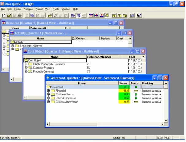
Oros of ABC Technologies
ABC’s core product is OROS4, an integrated set of the activity-based software applications that allow companies to track and to manage their critical activity information. The OROS modules are designed to work with one another to provide an integrated solution for implementing business improvements.
Oros Quick is an evaluation version of OROS ABC Plus module. The Oros Quick desktop is depicted in Fig. 4.3.
3BPwin is the software package of Computers Associates for the BP mapping into the IDEF models
CHAPTER 5. ANALYTICAL BP MODELING 5.1. Steps of the analytical modeling
The principle advantage of the analytical modeling is that it leads to the general results, whereas the simulation results are specific for a simulation run. Let us consider the steps of creating analytical models, Fig. 5.1.
Creating a conceptual model of the problem
in question
Selecting an appropriate mathematical
scheme
Creating a mathematical model
Choosing analytical methods for estimating
the model parameters
Conducting experiments with the analytical
model and analyzing the results
Figure 5.1. Creating a mathematical model
Since the activities are the basic BP elements, the conceptual BP model is “responsible” for representing their order and logic of execution. Once created, the conceptual
model tends to become a formalized one. As far as the IDEF3 standard is concerned, we can state that due to its formalism and high expressive power it constitutes a solid ground for creating the BP analytical models.
5.2. Classification of the BP models
The BP models are classified into deterministic and stochastic. The models that contain no random variables are deterministic. A stochastic model has one or more random variables either as an input or as a model parameter.
In the deterministic framework, the order and the conditions of the activity execution are assumed to be invariable. That implies an invariable customer routing and an invariable service procedure, specifically, constant service time.
In the stochastic framework, a BP model presumes no pattern for either the order of activity executing or the service procedure.
Deterministic or Stochastic Routing Stochastic C & T
P
Deterministic C & TD
Deterministic RD
Stochastic RP
Deterministic or Stochastic BP model: Time & Cost (T&C) parameters
According to this classification, we can distinguish the following four groups of the BP models: C T RD D & DRPT&C C T RD P & PRPT&C
These groups define the adequate mathematical schemes. and denote the deterministic and the stochastic
R
D PR
BP routing respectively; and denote the deterministic and the stochastic
C T&
P DT&C temporary and cost BP parameters respectively.
5.3. Deterministic BP models DRDT&C
Appropriate mathematical schemes for this class of the BP model include the methods of dynamic and mathematical programming.
The initial statement of the activity execution order is usually stated in the form of the following table (Tab. 5.1.):
Table 5.1. Activity execution order Activity denotation Predecessors Activity Duration
а1 No 2 а2 No 1 а3 No 1 а4 No 2 а5 а1 2 а6 а2 3 а7 а1 4 а8 а3, а6 1 а9 а4, а5, а8 1
The IDEF3 model (Fig. 5.3) and the corresponding graph model (Fig. 5.4.) are directly derived from Tab. 5.1.
Figure 5.3.IDEF3 model of the activities (screenshot: BPwin ®)
a
1a
2a
3a
5a
6a
4a
7a
8a
9(1)
(2)
(3)
(4)
(5)
(0)
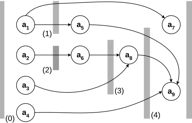
Converting the BP model into the network graph is less trivial and requires some explanation. The nodes of the network graph represent states and the arcs (state transitions) denote activities. The node on the network graph is a i state of the BP model, which corresponds to the completion of all activities denoted by the graph arcs that are entering the state . The arc corresponds to the i ij activitybetween the adjacent states i and j. Thus, the BP graph model, which is represented in Fig. 5.4., has six states marked with numbers in brackets. The state (0) corresponds the BP beginning and the state (5) is the BP ending. At the state (1) the activity completes and the activities and are allowed to start. At the state (3) the activities and complete and the activity is allowed to start. However, since takes shorter time to complete than + , the start of “floats” within certain bounds while “waiting” for the completion of + (float start time).
1 a a5 a7 6 a a3 a8 3 a a2 a6 a3 2 a a6
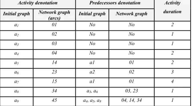
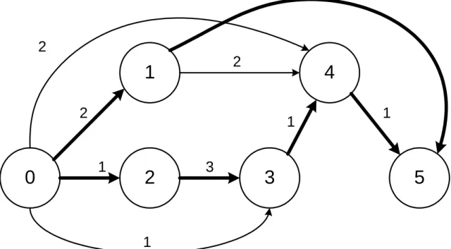
As a result, both the IDEF3 model on Fig. 5.3 and the initial graph model on Fig. 5.4 can be transformed to the network graph with 6 nodes (states) numbered from 0 through 5, see Fig. 5.5. The mapping of the initial graph of activities on the network graph is shown in Tab 5.2.
Table 5.2. Mapping of the initial graph of activities on the network graph Activity denotation Predecessors denotation
Initial graph Network graph
(arcs) Initial graph Network graph
Activity duration а1 01 No No 2 а2 02 No No 1 а3 03 No No 1 а4 04 No No 2 а5 14 а1 01 2 а6 23 а2 02 3 а7 15 а1 01 4 а8 34 а3, а6 03, 23 1 а9 45 а4, а5, а8 04, 14, 34 1
If we represent the network graph (Fig. 5.5) as a Gantt chart, it will be clear that there have to be at least four executors (units that execute individual activities) to run the BP. Here we do not consider any conflicts arising from one executor (a unit that executes an activity) allocated to several activities, i.e. there always exist sufficient (= infinite or equal to the total number of the activities) number of executors.
1
0
2
3
4
5
2
1
2
1
3
2
4
1
1
Figure 5.5. Network graph of the activities. Activities 03, 04, 14 have float start times
5.3.1. Bellman’s dynamic programming for the BP scheduling
ij
τ is the duration of the activity ij;
* i
t is the earliest moment of time when the event occurs; i *
* i
t is the latest moment of time when the event i occurs;
ij
r is the float start time of the activity ij.
The meaning of these terms is as follows:
* i
t is the earliest possible moment when the event occurs subject to the sequence order of the activities;
i
* * i
t is the latest moment when the event i occurs subject to the BP completion time equality;
ij
r is the float start time for the activity ij defined by ) ( * * * ij i j ij t t r = − +τ . (5.1)
The problem is to derive the schedule from the graph by computing the above introduced schedule parameters.
In terms of the network planning, we need to find out the critical (longest) path on the network graph. The activities that belong to the critical path determine the BP execution (completion time).
0 → 1 → 4 → 5 0 → 4 → 5 0 → 1 → 5
0 → 2 → 3 → 4 → 5 0 → 3 → 4 → 5
Hence, the critical path method leads to the following expression for the total BP execution time: )} ( ), ( ), ( ), ( ), {( max 45 34 03 45 34 23 02 15 01 45 04 45 14 01 τ τ τ τ τ τ τ τ τ τ τ τ τ τ + + + + + + + + + = Σ T
Generally, the network graph structure is usually too complicated for deriving such an expression. An appropriate body of mathematics for solving the task is Bellman’s dynamic programming [12].
Bellman’s method converts the task of computing the BP completion time into a sequence of standard steps defined as follows:
{
j ji}
i G j i t t = + +τ ∈ * ) ( * max , (5.2)where is the set of the nodes adjacent to the node i from left. For example, for the node 4: . ) (i G+ } 3 , 1 , 0 { ) 4 ( = + G
Equation (5.2) is used repeatedly for computing for each node starting from the node 0. The last step concludes computing of the BP completion time.
* i t
Also, the schedule parameter ** can be computed with Bellman’s method:
i t
{
i ji}
j G i j t t = − −τ ∈ * * ) ( * * min , (5.3)where is the set of the nodes adjacent to the node G−(j) j from right. For example, for the node 1: G−(1) = {4,5}.
Equation (5.3) is used repeatedly for computing for each node starting from the end node and moving backwards to the initial one.
* *
j t
For the case in question, the results of the BP scheduling analysis are graphically represented in Fig.5.6. The shortest BP execution time is: . is equal to the sum of the activities duration lying on each of the two critical paths: 0 → 1 → 5 or 0 → 2
→ 3 → 4 → 5 (bold arcs in Fig. 5.5). The activities out of the critical path have the following float start time:
6 * * 5 * 5 = = = Σ t t T TΣ . 1 , 2 , 3 04 14 03 = r = r = r
0
2
3
4
2
5
1
2
3
1
2
1
4
2
1
0 1 4 2 4 6 0 1 4 6 5 2 1 3 0 0 3 0 0 0 01
Duration of an activity0 The earliest occurrence of an event
0 The latest occurrence of an event 3 Float start time of an activity
5.3.2. BP scheduling as a problem of mathematical programming
Starting point
Suppose the order of the activity execution is given. The number of the activity executors is unlimited. So, the activities can start as soon as it is required.
The BP scheduling problem means revealing the actual start moments of each activity. Let us begin with the problem definition. We are expecting the results, which are the same as ones obtained in the pervious section with Bellman’s dynamic programming.
Notation ij
τ is the start time of the activity ij;
ij
T is the end time of the activity ; ij
ij
t is the duration of the activity ij. Obviously, Tij = τij + tij. Problem definition
{ }
{
0}
, (0), ) ( , ), ( ; 1 , 1 , , min 0 − + Σ + Σ ∈ = ∈ ⎭ ⎬ ⎫ + = ≤ ∈ − = ⎪⎭ ⎪ ⎬ ⎫ + = ≥ G k M G l t T T T i G l M i t T T to subject T k lM lM lM lM ij li li li ij τ τ τ τ (5.4)where , ) are the sets of the right-hand and the left-hand nodes adjacent to the node
) (j
G− G+(j
j on the BP network graph (see Fig. 5.5). TΣ is the BP total execution time.
M is the final event node number. Therefore, the total number of the graph nodes equals M +1.
The logic of the activity execution order is given in the form of a set of constraints. For instance, the inequality τij ≥Tli means that the activity ij does not start unless its predecessor activity li has finished.
⎪ ⎪ ⎪ ⎪ ⎪ ⎪ ⎪ ⎪ ⎪ ⎪ ⎪ ⎪ ⎪ ⎪ ⎪ ⎩ ⎪⎪ ⎪ ⎪ ⎪ ⎪ ⎪ ⎪ ⎪ ⎪ ⎪ ⎪ ⎪ ⎪ ⎪ ⎨ ⎧ = = = = + = + = ≤ + = + = ≤ + = + = ≥ + = + = ≥ + = + = ≥ + = + = ≥ + = + = ≥ + = + = ≥ + = + = ≥ ≥ Σ Σ Σ 0 4 1 1 2 2 1 3 1 2 , min 04 03 02 01 15 15 15 15 15 45 45 45 45 45 34 34 34 34 34 45 04 04 04 04 04 45 14 14 14 14 14 45 03 03 03 03 03 34 23 23 23 23 23 34 02 02 02 02 02 23 01 01 01 01 01 15 01 14 τ τ τ τ τ τ τ τ τ τ τ τ τ τ τ τ τ τ τ τ τ τ τ τ τ τ τ τ τ τ t T T T t T T T t T T t T T t T T t T T t T T t T T t T T T to subject T (5.5) Compacting (5.5) yields: ⎪ ⎪ ⎪ ⎪ ⎪ ⎪ ⎩ ⎪ ⎪ ⎪ ⎪ ⎪ ⎪ ⎨ ⎧ − ≤ − ≤ + ≥ + ≥ ≥ + ≥ ≥ ≥ ≥ Σ Σ Σ 4 1 1 2 1 3 1 2 2 , min 15 45 34 45 14 45 34 23 34 23 15 14 T T to subject T τ τ τ τ τ τ τ τ τ τ τ τ (5.6)
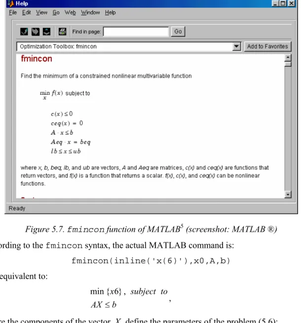
The problem defined as (5.4) is a typical problem of linear programming [13, 14]. The problem has six unknown variables. It is in the form ready for solving with an appropriate tool. Here we use MATLAB fmincon function (Optimization Toolbox) function, Fig. 5.7.
Figure 5.7. fmincon function of MATLAB5 (screenshot: MATLAB ®) According to the fmincon syntax, the actual MATLAB command is:
fmincon(inline('x(6)'),x0,A,b) It is equivalent to: b AX to subject x ≤ , } 6 { min , (5.7)
where the components of the vector X define the parameters of the problem (5.6): } , , , , , { } 6 , 5 , 4 , 3 , 2 , 1 { = 14 23 34 45 15 Σ = x x x x x x T X τ τ τ τ τ .
The matrix A and the vector are represented as the rows and columns in Tab 5.3. b
Table 5.3. Parameters of the problem
x1 x2 x3 x4 x5 x6 ≤ b -1 0 0 0 0 0 -2 0 0 0 0 -1 0 -2 0 -1 0 0 0 0 -1 0 1 -1 0 0 0 -3 0 0 -1 0 0 0 -1 1 0 0 -1 0 0 -2 0 0 1 -1 0 0 -2 0 0 0 1 0 -1 -1 0 0 0 0 1 -1 -4
Below is the dialog in MATLAB Command Window demonstrating how the problem is solved: A = [ -1 0 0 0 0 0; ... 0 0 0 0 -1 0; ... 0 -1 0 0 0 0; ... 0 1 -1 0 0 0; ... 0 0 -1 0 0 0; ... 1 0 0 -1 0 0; ... 0 0 1 -1 0 0; ... 0 0 0 1 0 -1; ... 0 0 0 0 1 -1]; b=[-2;-2;-1;-3;-1;-2;-2;-1;-4]; x0=[0;0;0;0;0;0]; fmincon(inline('x(6)'),x0,A,b) Active Constraints: 3 4 7 8 ans = 2 1 4 5 2 6
Here ans is the solution for the vector X defining the activities start time and the BP total
execution time: } 6 , 2 , 5 , 4 , 1 , 2 { } , , , , , { } 6 , 5 , 4 , 3 , 2 , 1 { = 14 23 34 45 15 = = x x x x x x TΣ X τ τ τ τ τ
This solution TΣ =6 coincides with one obtained using Bellman’s method (see Sec. 5.3.1). Suppose that each activity consumes one unit of resource from a limited resource pool. Then, having the solution X it is easy to calculate the resources occupied at every moment of time from the start to the very end of the BP. The procedure is as follows:
1. Compute the start time τij and the end time for each activity ij from the solution X;
ij T
2. Sort both time sets {τij} and {Tij} in ascending order;
3. Process these sets for the events of the release or the seizure of the BP executors. This is a way to get an insight into the utilization dynamics of executors as shown in Tab. 5.4. Note that the event “Activity Start” corresponds to seizing an executor, while the event “Activity Finish” corresponds to releasing an executor.
Table 5.4. Utilization dynamics of executors Event type
Event number
Event
time Activity Start (S) / Activity Finish (F) Change in the amount of the executors in use The amount of executors in use 1 10 S +1 1 2 15 S +1 2 3 16 S +1 3 4 22 S +1 4 5 27 F -1 3 6 31 F -1 2 7 33 S +1 3 8 34 F -1 2 9 38 F -1 1 10 45 S +1 2 11 50 S +1 3 12 56 S +1 4 13 57 F -1 3 14 58 F -1 2 15 70 S +1 3 16 73 S -1 2 17 81 F -1 1 18 98 F -1 0
5.3.3. BP resource optimization by means of mathematical programming
Starting point
Assume that the resources (activity executors) are identical and the activity execution order is given. A resource is seized by an activity for the total time of the BP execution. Therefore, a resource cannot be handed from one activity to another and the number of the resources cannot be less then the number of the activities. The actual problem is to minimize the number of the resources (executors) subject to the BP finishing in time.
Notation ij
m is the number of the resources assigned to the activity ij;
ij
τ is the activity ij start time;
ij
T is the activity ij end time;
ij
Q is the activity ij labor expenditures (e.g. man-hours);
ij
t is the activity ij duration (e.g. hours).
According to the meaning of the activity parameters:
ij ij ij ij ij ij m Q t T =τ + =τ + .
The problem of the resources optimization can be stated as follows: ( )
{
{
0}
, (0), ) ( , ), ( ; 1 , 1 , , min 0 − + Σ + ∈ = ∈ ∀ ∈ ⎪ ⎭ ⎪ ⎬ ⎫ + = ≤ ∈ − = ⎪ ⎭ ⎪ ⎬ ⎫ + = ≥ ⎭ ⎬ ⎫ ⎩ ⎨ ⎧∑
G k N m ij M G l m Q T T T i G l M i m Q T T to subject m k ij lM lM lM lM lM li li li li li ij ij ij τ τ τ τ (5.8)where , are the sets of the right-hand and the left-hand nodes adjacent to the node on the BP network graph.
) (j
G− G+(j)
j M is the final event node number; N is the set of the integer numbers. For the graph model in Fig. 5.5, the problem definition is the following:
⎪ ⎪ ⎪ ⎪ ⎪ ⎪ ⎪ ⎪ ⎪ ⎪ ⎪ ⎪ ⎪ ⎪ ⎪ ⎩ ⎪⎪ ⎪ ⎪ ⎪ ⎪ ⎪ ⎪ ⎪ ⎪ ⎪ ⎪ ⎪ ⎪ ⎪ ⎨ ⎧ ∈ = = = = + = ≤ + = ≤ + = ≥ + = ≥ + = ≥ + = ≥ + = ≥ + = ≥ + = ≥ ≥ + + + + + + + + Σ Σ = N m m m m m m m m m m Q T T T m Q T T T m Q T T m Q T T m Q T T m Q T T m Q T T m Q T T m Q T T T m m m m m m m m m 45 34 23 15 14 04 03 02 01 04 03 02 01 15 15 15 15 15 45 45 45 45 45 34 34 34 34 34 45 04 04 04 04 04 45 14 14 14 14 14 45 03 03 03 03 03 34 23 23 23 23 23 34 02 02 02 02 02 23 01 01 01 01 01 15 01 14 45 34 23 15 14 04 03 02 01 , , , , , , , , 0 , , , , , , , , , ) ( min τ τ τ τ τ τ τ τ τ τ τ τ τ τ τ τ τ τ τ τ τ (5.9)
The problem definition (5.9) includes 14 unknown variables. Nine variables are of the type, i.e. the arguments of the objective function. Five variables
ij
m τ14, τ15, τ23, τ34, τ45
define the BP scheduling.
The problem (5.9) can be solved with MATLAB Optimization Toolbox. As it belongs to the class of nonlinear programming [14], fseminf function has to be employed, Fig. 5.8.
Figure 5.8. fseminf function of MATLAB (screenshot: MATLAB ®)
The final solution of problem (5.9) is obtained by iterations of the constrained nonlinear programming. The intermediate solutions are to be analyzed for the non-integer values of . These are to be set to the nearest integer values. Such a solution is considered as sub-optimal and it is a starting point for further improvements.
ij
5.4. Stochastic BP models: DRPT&C and PRPT&C
5.4.1. DRPT&C model
Consider the following two problem definitions of the BP scheduling for the model:
C T RP D &
1. The variance of the activities duration is so small that it does not change the critical paths;
2. The variance of the durations is large enough to change the critical paths.
Unchanged critical path
Both dynamic and mathematical programming methods are appropriate for this case. Note that the deterministic duration time of an activity has to be substituted with the corresponding mean value, i.e. the expectation E(tij) of the activity ij duration . tij
According to the probability theory [11], the expectation of the BP completion time equals the sum of the expectations of the activities
) (TΣ
E 6, which belong to the critical path:
∑
∈ Σ = path critical ij ij t T E( )Moreover, if all are independent variables, the variance tij V(TΣ) is given by:
∑
∈ Σ = path critical ij ij t V T V( ) ( ).Due to the central limit theorem [11], the sum of a large number of independent random variables subject to the same distribution will tend to the normal distribution. Hence, having expectation and variance values of an activity duration it is easy to find out the probability whether the BP completion time belongs to a given interval.
} ) (
{ TΣ −E TΣ ≤ε
P is the probability that the absolute value of the difference between the expectation E(TΣ) and its statistical estimate TΣ is no more than ε, where 2ε is the width of the confidence interval with the center at the point TΣ.
To compute P{ TΣ −E(TΣ) ≤ε} one has to use the cumulative normal distribution tables (also known as the Laplace integral tables) [11]:
6 This result holds for any random variables, whereas the variance (dispersion) of the sum of random variables equals the sum of the individual variances only if the variables are independent
) ) ( ( 2 } ) ( { Σ Σ Σ − ≤ = Φ T V T E T P ε ε , where dt e x x t
∫
− = Φ 0 2 2 2 1 ) ( π is the tabulated Laplace Integral.In case there are several critical paths, one can use a stricter approach. Thus, in Fig 5.5 the graph model of the BP has two critical paths. Therefore, the probability of the BP guaranteed completion within certain period of time can be computed as follows:
}] { 1 [ }] { 1 [ } {T ≤TΣ = −P T 1 >TΣ −P T 2 >TΣ P crit crit ,
where Tcrit1and Tcrit2 are the lengths of the corresponding critical paths.
Note that the probabilities and are computed with the assumption that and are normally distributed.
} {T 1 >TΣ P crit P{Tcrit2 >TΣ} 1 crit T Tcrit2
Let us supplement our case study with the variance of the activities duration, Tab. 5.5. Table 5.5. Variance of the activities duration
Duration Dispersion measure
Activity
mean min max variance st. dev. halfwidth
01 2.00 0.77 3.23 0.50 0.71 1.23 02 1.00 0.05 1.95 0.30 0.55 0.95 03 1.00 0.05 1.95 0.30 0.55 0.95 04 2.00 0.77 3.23 0.50 0.71 1.23 14 2.00 0.77 3.23 0.50 0.71 1.23 23 3.00 1.55 4.45 0.70 0.84 1.45 15 4.00 2.27 5.73 1.00 1.00 1.73 34 1.00 0.05 1.95 0.30 0.55 0.95 45 1.00 0.05 1.95 0.30 0.55 0.95
Computing the variances, we have:
5 . 1 0 . 1 5 . 0 } {Tcrit1 = + = V ; 6 . 1 3 . 0 3 . 0 7 . 0 3 . 0 } {Tcrit2 = + + + = V .
The expectation of the BP execution time is:
6 2 1 = = = Σ Tcrit Tcrit T .
Let us calculate the probability that the BP execution time is less than 8. For the normally distributed Tcrit1 and Tcrit2 we obtain:
051 . 0 449 . 0 5 , 0 ) 633 . 1 ( 5 , 0 ) 5 . 1 6 8 ( 5 , 0 } 8 {Tcrit1 > = −Φ − ≈ −Φ = − = P , 057 . 0 443 . 0 5 . 0 ) 581 . 1 ( 5 , 0 ) 6 . 1 6 8 ( 5 . 0 } 8 {Tcrit2 > = −Φ − ≈ −Φ = − = P . Hence, P{TΣ ≤8} = (1−0.051)(1−0.057)=0.895.
5.4.1.1. BP scheduling analysis with Crystal Ball
Let us consider another approach to the problem of computing the probability that the BP is completed within certain period of time. Here we will use Crystal Ball7, a software tool that employs the Monte-Carlo method also known as the method of statistical testing.
Let the duration of an activity be uniformly distributed as defined in Tab. 5.5. A dialogue window for setting uniformly distributed duration of the activities is shown in Fig. 5.9.
Figure 5.9. Setting the uniformly distributed duration of activities (screenshot: CrystalBall ®) The results of two independent experiments are the distributions and shown in Fig. 5.10 and 5.11. Each experiment consists of 1000 runs. We can see that
and 1 crit T Tcrit2 055 . 0 } 8 {Tcrit1 > = P P{Tcrit2 >8}=0.057. Therefore, P{TΣ ≤8}=0.945⋅0.943≈0.891.
7 Crystal Ball is the registered trade mark of Decisioneering Inc., [www.decisioneering.com]
Figure 5.10. Distribution of the duration for the first critical path. The uniform distribution case (screenshot: CrystalBall ®)
Figure 5.11. Distribution of the duration for the second critical path. The uniform distribution case (screenshot: CrystalBall ®)
Let us change the duration distributions from uniform to normal with the same mean and variance. The resulting histograms for each of the critical paths are represented in Fig. 5.13 and 5.14. According to the histograms we obtain: and
. Finally, 048 . 0 } 8 {Tcrit1 > = P 065 . 0 } 8 {Tcrit2 > =
P P{TΣ ≤8} = 0.952⋅0.935≈ 0.890. These results comply with ones obtained using the central limit theorem.
Figure 5.12. Setting the normally distributed duration of activities (screenshot: CrystalBall®)
Figure 5.13. Distribution of the duration for the first critical path. The normal distribution case (screenshot: CrystalBall ®)
Figure 5.14. Distribution of the duration for the second critical path. The normal distribution case (screenshot: CrystalBall ®)
Let us take a closer look at stating the tasks in the built-in Excel8 Crystal Ball environment. For our example the critical path method leads to the following expression for the BP completion time:
)} ( ), ( ), ( ), ( ), {( max 45 34 03 45 34 23 02 15 01 45 04 45 14 01 τ τ τ τ τ τ τ τ τ τ τ τ τ τ + + + + + + + + + = Σ T
The same function is set in an Excel cell for Crystal Ball in the following way:
Σ
T = MAX((D2+D6+D10);(D5+D10);(D2+D10);(D3+D7+D9+D10);(D4+D9+D10)). Here the cells D2 – D10denote the stochastic arguments τij of the Excel MAX function.
The simulation results in the form of the histograms representing the BP completion time are shown in Fig. 5.15 and 5.16 for the uniform and the normal distribution of the activities duration. We can see that the probability of the BP completing in time almost does not depend on the type of the activities duration distribution. Thus, for the uniform distribution we have: , though for the normal distribution we obtain almost the same result: .
942 . 0 } 8 {TΣ ≤ ≈ P 937 . 0 } 8 {TΣ ≤ ≈ P
Figure 5.15. Simulation results for the uniform distribution (screenshot: CrystalBall®)
Figure 5.16. Simulation results for the normal distribution (screenshot: CrystalBall ®)
5.4.2. Stochastic PRPT&C models with an account for the resource utilization
Let us return to the BP IDEF3 model and complement it with a resource reference using the so called Reference Objects of the IDEF3 syntax. For our case study, when the resources are taken into account, the initial IDEF3 model (Fig. 5.3) becomes one shown in Fig. 5.17. Each activity is assigned to the one of the BP resources D1 – D4.
Suppose that the duration of an activity means the net time of the activity processing. For that kind of the BP model, we consider a resource as a serving system with a queue of “customers”. A “customer” has an “order” for an activity execution.
Figure 5.17. IDEF3 model with resources (screenshot: BPwin ®)
Having this in mind, we conclude that the waiting time in queues has to be taken into account when calculating the BP completion time. This is a good reason for applying the queueing theory as a basis of the BP analytical modeling.
5.4.2.1. BP PRPT&C model in the form of the queueing network
Fundamentals
The inhomogeneous networks with infinite queues are suitable for BP modeling. A queueing network is a network of queues. In other words, a queueing network is a set of nodes, where a node is a serving system with a queue of customers at its entrance. Once entering a network, the customers of the system are routed from one node to another receiving service at each node and, finally, leaving the network. An open network receives customers from an outside independent source. A leaving customer is interpreted as the order which has been fulfilled or a client which has been served.
M/G/1 – inhomogeneous customer flow at the entrance
Incoming customers are inhomogeneous because they arrive at different rates and need different time of serving.
In terms of the queuing theory, a serving system has an inhomogeneous customer incoming flow summing the flows with the rates λ1,λ2, ...λn. Each of them is the flow of Poisson’s (exponential) arrivals. The customers from the flow i are served according to the general (i.e. arbitrary)distribution with the mean xi and the variance , see Fig. 5.18. Vi
N 1
.
.
.
λ
λ
M/G/1x
1,..
x
NFigure 5.18. Model of a serving system
It is known [6] that the mean waiting time in the queue, , is the same for each incoming flow of customers and is given by:
Q w R T wQ − = 1 0 , (5.10)
( )
[
i i]
N i i x V T =∑
+ = 2 1 0 2 1 λ , (5.11) i i i N i i x R=∑
ρ ρ = λ = , 1 , (5.12)where T0 denotes the mean remaining service time for the customer occupying the server. The parameter R has a sense of the utilization of the server loaded with the inhomogeneous customer flow. The condition Rj <1 is required for the serving system to be stable.
According to the BP modeling application, we consider each resource (the reference object of the IDEF3 model, Fig. 5.17) as a single-channel serving system M/G/1. Since a resource object is shared by several activities (D1, D2, D3, and D4 in Fig. 5.17), the serving system has customers of various classes at the entrance. The number of classes is equal to the number of the activities within the BP IDEF3 model.
Inhomogeneous open network of single-server queues
While the rigorous coverage of the queueing networks is beyond the scope of the book, the main concepts are outlined below.
Let us consider a stable system with an infinite calling population9 and no limit on the system capacity. We can obtain the following results [2]:
1. Provided no customers are created or destroyed in the queue, on the average (i.e. over the long run) the queue outcoming rate is the same as the incoming one;
2. The customers are able to change their class by routing from one queue to another; 3. If the customers of class l arrive to queue i at rate λil and the fraction 0≤ pil,jk ≤1 of them are routed to queue j upon their transformation to class , then on the average the arrival rate of the class k from the queue to the queue
k
i j is λjk =λilpil,jk;
4. The overall arrival rate of the class l into the queue j, λjl, is the sum of the arrival rate from all sources. If the customers arrive from the outside of the network at the rate λ0, then: N k M j p p N l jk il il M i jk o jk , 1, , 1, 1 , 1 , 0 + = = =
∑
∑
= = λ λ λ , (5.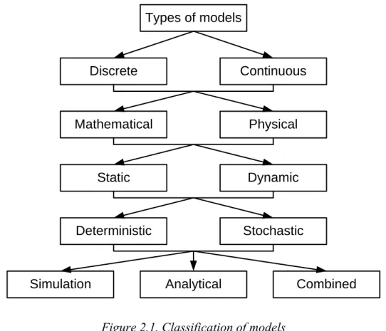

![Figure 4.1. Structure of the traditional cost system (based on [3], p.83)](https://thumb-us.123doks.com/thumbv2/123dok_us/657314.2579239/23.892.157.698.103.782/figure-structure-traditional-cost-based-p.webp)
![Figure 4.2. Structure of the ABC system (based on [3], p. 84)](https://thumb-us.123doks.com/thumbv2/123dok_us/657314.2579239/24.892.251.669.148.819/figure-structure-abc-based-p.webp)