Independent Comparative Study of PCA, ICA, and LDA
on the FERET Data Set
Kresimir Delac, Mislav Grgic, Sonja Grgic
University of Zagreb, FER, Unska 3/XII, Zagreb, Croatia
Received 28 December 2004; accepted 27 February 2006
ABSTRACT: Face recognition is one of the most successful applica-tions of image analysis and understanding and has gained much attention in recent years. Various algorithms were proposed and research groups across the world reported different and often contra-dictory results when comparing them. The aim of this paper is to present an independent, comparative study of three most popular appearance-based face recognition projection methods (PCA, ICA, and LDA) in completely equal working conditions regarding prepro-cessing and algorithm implementation. We are motivated by the lack of direct and detailed independent comparisons of all possible algo-rithm implementations (e.g., all projection–metric combinations) in available literature. For consistency with other studies, FERET data set is used with its standard tests (gallery and probe sets). Our results show that no particular projection–metric combination is the best across all standard FERET tests and the choice of appropriate projec-tion–metric combination can only be made for a specific task. Our results are compared to other available studies and some discrepan-cies are pointed out. As an additional contribution, we also introduce our new idea of hypothesis testing across all ranks when comparing performance results. VVC 2006 Wiley Periodicals, Inc. Int J Imaging Syst Technol, 15, 252–260, 2005; Published online in Wiley InterScience (www.interscience.wiley.com). DOI 10.1002/ima.20059
Key words: face recognition; PCA; ICA; LDA; FERET; subspace analysis methods
I. INTRODUCTION
Over the last ten years or so, face recognition has become a popular area of research in computer vision and one of the most successful applications of image analysis and understanding. Because of the nature of the problem, not only computer science researchers are interested in it, but also neuroscientists and psychologists. It is the general opinion that advances in computer vision research will pro-vide useful insights to neuroscientists and psychologists into how human brain works, and vice versa. A general statement of the face recognition problem can be formulated as follows (Zhao et al., 2003): Given still or video images of a scene, identify or verify one or more persons in the scene using a stored database of faces. A
sur-vey of face recognition techniques has been given by Zhao et al., (2003). In general, face recognition techniques can be divided into two groups based on the face representation they use:
1. Appearance-based, which uses holistic texture features and is applied to either whole-face or specific regions in a face image;
2. Feature-based, which uses geometric facial features (mouth, eyes, brows, cheeks etc.) and geometric relationships between them.
Among many approaches to the problem of face recognition, appearance-based subspace analysis, although one of the oldest, still gives the most promising results. Subspace analysis is done by projecting an image into a lower dimensional space (subspace) and after that recognition is performed by measuring the dis-tances between known images and the image to be recognized. The most challenging part of such a system is finding an adequate subspace.
In this paper, three most popular appearance-based subspace projection methods for face recognition will be presented, and they will be combined with four common distance metrics. Projection methods to be presented are: Principal Component Analysis (PCA), Independent Component Analysis (ICA), and Linear Discriminant Analysis (LDA). PCA (Turk and Pentland, 1991) finds a set of the most representative projection vectors such that the projected sam-ples retain most information about original samsam-ples. ICA (Bartlett et al., 2002; Draper et al., 2003) captures both second and higher-order statistics and projects the input data onto the basis vectors that are as statistically independent as possible. LDA (Belhumeur et al., 1996; Zhao et al., 1998) uses the class information and finds a set of vectors that maximize the between-class scatter while minimizing the within-class scatter. Distance metrics used are L1 (City block), L2 (Euclidean), cosine and Mahalanobis distance.
The aim of this paper is to provide an independent, comparative study of these three projection methods and their accompanied dis-tance metrics in completely equal working conditions. In order to perform a fair comparison, same preprocessed images are the input into all algorithms and the number of dimensions to be retained is chosen following the standard recommendations. For consistency
with other studies, FERET data set (Phillips et al., 2000), with its standard test sets, is used for comparisons. This research is motivated by the lack of direct and detailed comparisons of these three projec-tion methods. They are rarely compared in a single paper and almost never are all possible implementations considered (e.g., all projec-tion–metric combinations). It is interesting to notice that the findings of other research groups are often contradictory on this subject and this is another important reason for performing a study of this kind. For example, Liu and Wechsler (1999) and Bartlett et al. (2002) claim that ICA outperforms PCA, while Baek et al. (2002) claim that PCA is better. Moghaddam (2002) states that there is no significant difference. Beveridge et al. (2001a) claim that in their tests LDA per-formed uniformly worse than PCA, Martinez and Kak (2001) state that LDA is better for some tasks, and Belhumeur et al. (1996) and Navarrete and Ruiz-del-Solar (2002) claim that LDA outperforms PCA on all tasks in their tests (for more than two samples per class in training phase). All these results are in most cases given only for one or two projection–metric combinations for a specific projection method, and in some cases using nonstandard databases or some hybrid test sets derived from a standard database.
The rest of this paper is organized as follows: Section II gives a brief description of the algorithms to be compared, Section III reports the details of methodology, Section IV presents the results and compares our results to results of other research groups and Section V concludes the paper.
II. ALGORITHMS
Even though projection methods and metrics used in this work are already well known, we will include a brief description for the sake of completeness. All three projection methods are so called sub-space analysis methods. A 2D imageGwithmrows andncolumns
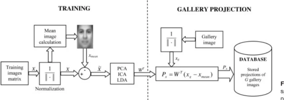
can be viewed as a vector (after concatenating its rows or columns) inNdimensional image space (RN¼mn). Since space derived this way is highly dimensional, recognition in it is unfeasible. There-fore, recognition algorithms usually derive lower dimensional spaces to do the actual recognition while retaining as much infor-mation (energy) from the original images as possible. We will fur-ther clarify this on the example from this research: the original FERET images (after preprocessing) are the size of 6050 pixels, thus the image space dimensionality isRN¼6050¼3000. It will be shown that projection methods presented here will yieldR270(R224 for LDA) subspace in which the recognition will be done and in these 270 dimensions 97.85% of original information (energy) is retained. An example of building a general subspace appearance-based face recognition system can be seen in Figure 1. Training of the subspace system can be seen in the left part of the figure and the procedure for projecting gallery images onto a subspace (projection matrixWT) can be seen in the right part of the figure;Xis a matrix containing the images expressed as vectors in its columns,xmean–
mean image (as a vector),X~– matrix containing mean-subtracted images in its columns,WT– projection matrix,xg– gallery image
(as a vector). During the training phase, the projection matrix (con-taining the basis vectors of the subspace) is calculated and then the gallery images (the images of known persons) are projected onto that subspace and their projections are stored in a database. Later, in the matching phase (Fig. 2), new image is normalized, mean-sub-tracted, projected onto the same subspace as the gallery image was and its projection is then compared to stored gallery projections (thenearest neighboris determined by calculating the distancesd
from a probe image projection to all gallery images projections and then choosing the minimum distance as a similarity measure). The identity of the most similar gallery image is then chosen to be the
Figure 1. An illustration of general sub-space appearance-based face recog-nition system.
Figure 2. The matching phase of a general subspace face recognition system.
result of recognition and the unknown probe image is identified. It is important to mention that a general face recognition system can work in two modes: (1) theidentification modewhere the input to the system is an unknown face and the system reports back the determined identity (our case) and (2) theverification modewhere the system needs to confirm or reject the claimed identity of the input face. All our experiments are conducted for the identification mode and the general illustration of the systems shown in Figures 1 and 2 illustrates our experiments.
A. Principal Component Analysis (PCA). In our experiments we implemented Principal Component Analysis (PCA) procedure as described by Turk and Pentland (1991). Given ans-dimensional vector representation of each face in a training set ofM images, PCA tends to find a t-dimensional subspace whose basis vectors correspond to the maximum variance direction in the original image space. This new subspace is normally lower dimensional (ts). New basis vectors define a subspace of face images called face space. All images of known faces are projected onto the face space to find sets of weights that describe the contribution of each vector. To identify an unknown image, that image is projected onto the face space as well to obtain its set of weights. By comparing a set of weights for the unknown face to sets of weights of known faces, the face can be identified. If the image elements are considered as ran-dom variables, the PCA basis vectors are defined as eigenvectors of the scatter matrixSTdefined as:
ST¼ XM
i¼1
ðxiÞ ðxiÞT ð1Þ
whereis the mean of all images in the training set (themean face, Fig. 1) andxiis theith image with its columns concatenated in a
vec-tor. The projection matrixWPCAis composed ofteigenvectors
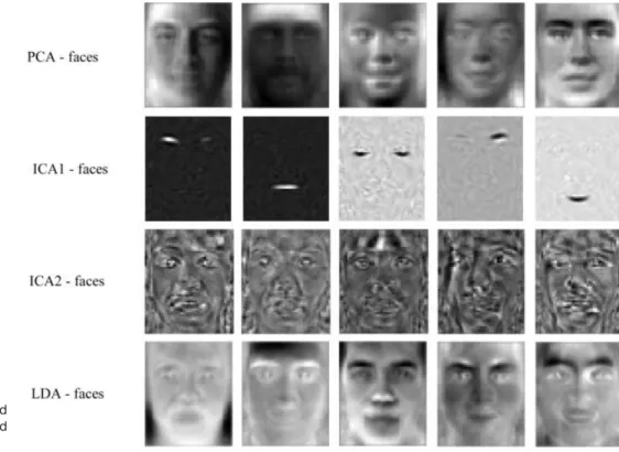
corre-sponding totlargest eigenvalues, thus creating at-dimensional face space. Since these eigenvectors (PCA basis vectors) look like some ghostly faces they were conveniently namedeigenfaces(Fig. 3).
B. Independent Component Analysis (ICA). PCA considered image elements as random variables with Gaussian distribution and minimized second-order statistics. Clearly, for any non-Gaussian distribution, largest variances would not correspond to PCA basis vectors. Independent Component Analysis (ICA) (Bartlett et al., 2002; Draper et al., 2003) minimizes both second-order and higher-order dependencies in the input data and attempts to find the basis along which the data (when projected onto them) arestatistically in-dependent. Bartlett et al. (2002) provided two architectures of ICA for face recognition task:Architecture I– statistically independent basis images (ICA1 in our experiments) andArchitecture II– facto-rial code representation (ICA2 in our experiments).
Our implementation of ICA uses the INFOMAX algorithm pro-posed by Bell and Sejnowski and used by Bartlett et al. (2002). PCA is used to reduce dimensionality prior to performing ICA.
C. Linear Discriminant Analysis (LDA). Linear Discriminant Analysis (LDA) (Belhumeur et al., 1996; Zhao et al., 1998) finds the vectors in the underlying space that best discriminate among classes. For all samples of all classes the between-class scatter matrixSBand
the within-class scatter matrixSWare defined by:
SB¼ Xc i¼1 Mi ðxiÞ ðxiÞT ð2Þ SW¼ Xc i¼1 X xkXi ðxkiÞ ðxkiÞ T ð3Þ whereMiis the number of training samples in classi,cis the
num-ber of distinct classes,iis the mean vector of samples belonging
to classiandXirepresents the set of samples belonging to classi
withxkbeing thek-th image of that class.SWrepresents the scatter
of features around the mean of each face class andSBrepresents the
scatter of features around the overall mean for all face classes.
Figure 3. Face representations found by PCA (eigenfaces), ICA1, ICA2, and LDA.
The goal is to maximize SB while minimizing SW, in other
words, maximize the ratio det|SB|/det|Sw|. This ratio is maximized
when the column vectors of the projection matrix (WLDA) are the
eigenvectors ofSW1SB. In order to preventSWto become singular,
PCA is used as a preprocessing step and the final transformation is
WoptT¼WLDATWPCAT.
In Figure 3 PCA-faces (eigenfaces), ICA1-faces, ICA2-faces,
andLDA-facescan be seen. Theseghostly facesare basis vectors produced by projection methods, reshaped to a matrix form of the original image size for convenience. This is a good illustration of the differences between subspaces derived by each of those projec-tion methods. If we take a closer look at the basis vector representa-tions it can be seen that PCA, LDA, and ICA2 produce global fea-tures; every image feature is influenced by every pixel. ICA1 pro-duces spatially localized features that are only influenced by small parts of an image, thus isolating particular parts of faces. Logical conclusion is that ICA1 should be optimal for recognizing facial actions and suboptimal for recognizing temporal changes in faces or images taken under different illumination conditions. This theo-retical property of ICA1 will be proven by our experiments.
D. Distance Measures. Four different distance measures will be used in comparisons: L1, L2, cosine angle (COS), and Mahalanobis distance (MAH). Generally, for two vectors,xandy, distance meas-ures are defined as:
dL1ðx;yÞ ¼ jxyj ð4Þ
dL2ðx;yÞ ¼ kxyk
2 ð
5Þ
dcosðx;yÞ ¼ kxk kykxy ð6Þ
dMAHðx;yÞ ¼
ffiffiffiffiffiffiffiffiffiffiffiffiffiffiffiffiffiffiffiffiffiffiffiffiffiffiffiffiffiffiffiffiffiffiffiffiffiffi
ðxyÞV1ðxyÞT q
ð7Þ whereVis the covariance matrix. In the rest of this paper, we will address the specific projection–metric combination as analgorithm. Since we implemented four projection methods (PCA, ICA1, ICA2, and LDA) and four distance measures (L1, L2, COS, and MAH), it can be concluded that we will effectively compare 16 different algorithms.
III. METHODOLOGY
A. Data. For consistency with other studies, we used the standard FERET data set including the data partitions (subsets) for recogni-tion tests, as described in Phillips et al., 2000. Thegalleryconsists of 1,196 images and there are four sets of probe images (fb, fc,
dup1, anddup2) that are compared to thegalleryimages in recogni-tion stage. Thefbprobe set contains 1,195 images of subjects taken at the same time asgalleryimages with one difference being that the subjects were told to assume a different facial expression. The
fcprobe set contains 194 images of subjects under different illumi-nation conditions. Thedup1(duplicate I) set contains 722 images taken anywhere between one minute and 1,031 days after the gal-leryimage was taken, anddup2(duplicate II) set is a subset ofdup1
containing 234 images taken at least 18 months after thegallery
image was taken. All images in the data set are of size 384256 pixels and grayscale.
B. Preprocessing. All algorithms and all image preprocessing steps were implemented in MATLAB1. Original FERET images were first spatially transformed (to get eyes at fixed points in
im-agery) based upon a ground truth file of eye coordinates supplied with the original FERET data. The standard imrotateMATLAB1 function was used with bilinear interpolation parameter. After that, all images were cropped the same way (using the eyes coordinates) to eliminate as much background as possible. No masking was done since it turned out that cropping eliminated enough background and the whole idea of this research was not to yield the best possible rec-ognition results but to fairly compare the algorithms. After cropping, images were additionally resized to be the size of 6050 using the standard MATLAB1imresize function with bilinear interpolation. Finally, image pixel values were histogram equalized to the range of values from 0 to 255 using the standardhisteqfunction.
C. Training. To train the PCA algorithm we used a subset of classes for which there were exactly three images per class. We found 225 such classes (different persons) in the FERET data set, so our training set consisted of 3225¼675 images (M¼675,
c¼225). PCA derived, in accordance with theory,M1¼ 674 meaningful eigenvectors. We adopted the FERET recommendation and kept the top 40% of those, resulting in 270-dimensional PCA subspace (40% of 674 270). It was calculated that 97.85% of original information (energy) was retained in those 270 eigenvec-tors. This subspace was used for recognition as PCA face space and as input to ICA and LDA (PCA was the preprocessing dimensional-ity reduction step). ICA yielded two representations (ICA1 & ICA2) using the input from PCA (as in Bartlett et al., 2002). Dimensionality of both ICA representations was also 270. How-ever, LDA yielded only 224-dimensional space since it, by theory, can produce a maximum ofc1 basis vectors. All of those were kept to stay close to the dimensionality of PCA and ICA spaces and thus make comparisons as fair as possible. After all the subspaces have been derived, all images from data sets were projected onto each subspace and recognition using nearest neighbor classification with various distance measures was conducted.
IV. RESULTS
Results of our experiment can be seen in Table I and Figure 4. We used two standard ways to present the results: (1) table showing algorithm performance at rank 1 (recognition rate within the top one match), and (2) Cumulative Match Score (CMS) curve (Phillips et al., 2000), showing the cumulative results for ranks 1 and higher. One interesting thing we noticed is the discrepancy in some cases between the rank 1 results and the CMS results when answering the question which algorithm performs better. It was noticed that the metric showing the best results at rank 1 did not always yield the best results at higher ranks. Five such cases were identified (most frequently for LDA) in this experiment. This can be seen in Table I by comparing the bolded best algorithm–metric combinations for rank 1 and the right two columns showing the best combinations at higher ranks. This brings to question any analyses done by compar-ing the CMS curves of those projection–metric combinations that yielded the best results at rank 1. This is why we decided to show the CMS curves for those metrics that produced best results at higher ranks for a specific algorithm.
A. Conclusions Based on a Specific Task. fb(thedifferent expressiontask). Even though ICA2þCOS combination produces the best results at rank 1 (Table I), LDAþCOS outperforms it from rank 6 further on (Fig. 4). Actually, ICA2þCOS performs uni-formly worse than other best projection–metric combinations at
higher ranks. But, it can be stated that the remaining three projec-tion–metric combinations (PCAþCOS, ICA1þL2, and LDAþCOS) produce similar results and no straightforward conclusion can be drawn regarding which is the best for this specific task. It stays unclear whether the differences between recognition rates for this task are statistically significant or not (we will address this issue in Section IV(C)). ICA1 performance was comparable to PCA and LDA and certainly better than ICA2. This confirms the theoretical property of ICA1 mentioned in Section II(C).
fc(thedifferent illuminationtask). ICA2þCOS wins here at rank 1 (Table I) but PCAþL1 is much better from rank 17 on (Fig. 4). ICA1 is the worst choice for this task. Again, this is not surprising since ICA1 tends to isolate the face parts and therefore should be bet-ter at recognizing facial actions than anything else.
dup1 & dup2(thetemporal changestasks). ICA2þCOS is the best here at every rank (as clearly illustrated in Fig. 4) and ICA1 is the worst. L1 norm seems to produce the best results for almost all other projection methods for this task and it is surprising that it is so rarely used in comparisons.
B. Metrics Comparison. L1 gives the best results in combina-tion with PCA across all four probe sets so it can be concluded that L2 distance metric is suboptimal for PCA (one exception being that COS outperforms L1 for the fb set, but statistical significance remains questionable). Following the same line of thought, it can be concluded that COS is superior to any other metric when used with ICA2. Actually, L2 is the best metric in only two combinations across all probe sets and projection methods. We found this result surprising since this was the most frequently used measure in the past. No clear conclusion can be drawn as to which metric works best with ICA1 and LDA and, at best, it can be stated that it depends on the nature of the task. This tells us that no combination of projection–metric for ICA1 and LDA are robust enough across
all tasks. MAH turned out to be the most disappointing metric in our tests and more variants of MAH distance calculations should be investigated (as in Beveridge et al., 2001a). If we analyze the best results given by the CMS, the metrics ranking looks something like this: L1 – 7 best results, COS – 6, L2 – 2, MAH – 1.
C. Evaluating the Differences in Algorithm Performance (Hypothesis testing). We think that, when comparing recogni-tion algorithms, it is important (yet often neglected) to answer the following question:when is the difference in performance statisti-cally significant?Clearly, the difference in performance of 1% or 2% could be due to pure chance, while 10% or more is probably not. We made our conclusions so far based on our intuitive analysis of the data (recognition rate percentage was higher or the curve on the plot appeared higher). However, we felt the need to investigate these intuitive presumptions using standard statistical hypothesis testing techniques. Generally, there are two ways of looking at the performance difference (Jambor et al., 2002): (1) determine if the difference (as seen over the entire set of probe images) is signifi-cant, (2) when the algorithms behave differently, determine if the difference is significant. As argued by Jambor et al. (2002 the first way to evaluate performance difference fails to take the full advant-age of the standard face recognition protocol, so we will focus on the second way and set our hypotheses like this:H1: when algo-rithms A and B differ on a particular image, A is more likely to cor-rectly identify that image,H0:when algorithms A and B differ on a particular image, they are equally likely to identify that image cor-rectly. In order to perform this test we recorded which of the four possible outcomes, when comparing two algorithms (SS– both suc-cessful,FF– both failed,FS– first one failed and the second one succeeded,SF– first one succeeded and the second one failed), is true for each probe image. Following the lead of Beveridge et al., 2001b; Jambor et al., 2002 we employed McNemar’s Test with the
Table I.Performance across four projection methods and four metrics.
Projection
Results at Rank 1 (%)
CMS Results Metric
L1 L2 MAH COS Highest Curve Same as Rank 1
Fb
PCA 82.26 82.18 64.94 81.00 PCAþCOS F
ICA1 81.00 81.51 64.94 80.92 ICA1þL2 T
ICA2 64.94 74.31 64.94 83.85 ICA2þCOS T
LDA 78.08 82.76 70.88 81.51 LDAþCOS F
Fc
PCA 55.67 25.26 32.99 18.56 PCAþL1 T
ICA1 18.04 17.53 32.99 12.89 ICA1þL1 F
ICA2 15.98 44.85 32.99 64.95 ICA2þCOS T
LDA 26.80 26.80 41.24 20.62 LDAþL2 F
Dup1
PCA 36.29 33.52 25.62 33.52 PCAþL1 T
ICA1 32.55 31.86 25.62 32.27 ICA1þL1 T
ICA2 28.81 31.99 25.62 42.66 ICA2þCOS T
LDA 34.76 32.96 27.70 33.38 LDAþL1 T
Dup2
PCA 17.09 10.68 14.53 11.11 PCAþL1 T
ICA1 8.97 7.69 14.53 8.97 ICA1þMAH T
ICA2 16.24 19.66 14.53 28.21 ICA2þCOS T
LDA 16.24 10.26 16.67 10.68 LDAþL1 F
Left part contains the results for rank 1 and the best projection–metric combinations are bolded. Right part contains are the best CMS results obtained by determining which metric gives the highest curve for a specific projection method at a specific probe set.
0.05 cutoff assumed. This test ignores the cases where both com-pared algorithms behave the same (SSorFF) and only uses the out-comes where they behave differently (SFandFS). LetnSFbe the
number of times theSFis observed andnFSthe number of timesFS
is observed. We are interested in the one-sided version of this test so the probability ofH0is bounded by:
PH0 XnFS i¼0 n! i!ðniÞ!0:5 n ð 8Þ wheren¼nSFþnFS. In other words,H0will be rejected in favor
ofH1ifPH00.05. So far, this test was usually performed only at
rank 1 so we decided to expand it to all ranks and to plot the results as a step curve (Figs. 5–8).
Using the described methodology we first checked if our choice of best metric for a specific projection method was correct. We con-firmed our choices of the highest curves and found that the choice was correct or, at least, that there is no significant difference between the chosen metric and the second best metric. Thus, the CMS curves compared in Figure 4 are truly the best choices of a projection–metric combination for a given task. Next, we plotted the decision graph based on McNemar’s Test (Figs. 5–8) for all CMS curves given in Figure 4. All possible comparison combina-tions are given thus yielding six plots for every probe set.
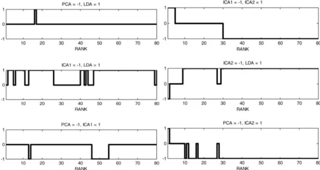
As expected, the most complicated situation is for thefbprobe set (Fig. 5). Here we claimed that LDAþCOS outperforms ICA2þCOS from rank 6 further on but this is obviously true only from rank 9
fur-ther on. For ofur-ther combinations we confirmed our presumption that there is no significant difference in performance (Fig. 5).
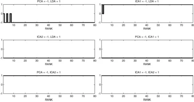
Situation is a little less complicated for thefcprobe set (Fig. 6). For example, we can see that there is no significant difference between ICA2þCOS and LDAþL2 from rank 25 on and yet the CMS curve in Figure 4 is always higher for ICA2þCOS. We also claimed that PCAþL1 is better than ICA2þCOS from rank 17 on. This is not quite true since it can be seen in Figure 6 that the difference becomes signifi-cant only from rank 27 further on. However, Figure 6 confirms the statement that ICA1 is the worst choice for this task.
It can be seen that fordup1(Fig. 7) anddup2set (Fig. 8) every-thing is relatively clear and all our previous conclusions are con-firmed by this test.
We can state that our previous overall conclusions regarding the relative performance were confirmed by this hypothesis testing technique and some new conclusions were drawn regarding the exact rank in which the differences become significant.
D. Comparison to Previous Work. It is worth mentioning at this point that most of the papers we will compare our results to do not use standard FERET test sets, but this should not be a problem since we will make the comparisons to their results based on the
relativeperformance.
First of all, we can state that our results are consistent to that of Phillips et al. (2000) regarding the relative ranking of probe sets. fb was found to be the easiest (highest recognition rates) and dup2 the hardest (lowest recognition rates). This is in clear
Figure 4. Cumulative Match Score (CMS curve) plots of best projection–metric combinations (the ones that yielded the highest curve when all metrics were compared for a specific algorithm) for a given probe set.
contradiction with Beak et al. (2002) who stated that fc is the hardest probe set. Also consistent with Phillips et al. (2000) is that LDAþCOS outperforms all others for the fbset (or at least that there is no significant difference). Both Phillips et al. (2000) and Draper et al. (2003), when comparing PCA and ICA, claim that ICA2 outperforms PCAþL2 and this is what we also have found. However, our detailed research also produced some new conclusions: (1) PCAþCOS outperforms ICA2þCOS forfbprobe set at higher ranks and (2) PCAþL1 outperforms ICA2COS for
fc probe set at higher ranks (this is also confirmed by hypothesis testing in Figs. 5–6). Those new conclusions are consistent to that
of Bartlett et al. (2002) who favor ICA2 over PCA (actually, mostly on difficult time-separated images), but we disagree with their claim that ICA2 is better for the different expression task also. As stated by Bartlett et al. (2002), we also found that ICA2 gives best results when combined with COS. Navarrete and Ruiz-del-Solar (2002) claim that LDAþCOS works better than PCA, which is certainly not the case here at rank 1 and is questionably true for higher ranks. We agree with Moghaddam (2002) who stated that there is no significant difference between PCA and ICA at rank 1, but we think that ICA is significantly worse at higher ranks.
Figure 5. Hypothesis testing for thefbprobe set—comparing the best projection–metric combinations from Figure 4. 1 or1 means that one or the other algorithm is significantly better at a given rank and 0 means that there is no significant difference.
Figure 6. Hypothesis testing for thefcprobe set—comparing the best projection–metric combinations from Figure 4. 1 or1 means that one or the other algorithm is significantly better at a given rank and 0 means that there is no significant difference.
Among the most surprising results was the poor performance of LDA in some cases. Contrary to FERET’s report in (Phillips et al., 2000) where the LDA implementation from UMD performed con-sistently better than the baseline PCA (Turk and Pentland, 1991), we found that this is not true in our experiments. However, the FERET test did not measure the effect that individual algorithm’s parts (components) have on overall performance and it did not con-cern with algorithm implementation details. One of the most impor-tant parts of design and implementation of an algorithm is the train-ing stage. It is unclear from Phillips et al., 2000 (and also from Zhao et al., 1998) exactly how was the LDA trained. Zhao et al. (1998) it is stated that the algorithm is trained using the 1038 FERET images
from 444 classes and in (Phillips et al., 2000) the baseline PCA was trained with randomly chosen 500 FERET images. These two dif-ferent training scenarios make it very difficult to directly compare these two algorithms and their various components. Even if we were to compare them, it is obvious that LDA should have a great advantage as it was trained with roughly two times bigger training set. The poor performance of our implementation of LDA could also be due to the relatively small training set. Similar problem was identified and researched in detail in Martinez and Kak, 2001 where it is concluded that when the training set is small, PCA can outper-form LDA. Another important thing to mention is that LDA is much more sensitive to different training sets than PCA or ICA. There is
Figure 7. Hypothesis testing for thedup1probe set—comparing the best projection–metric combinations from Figure 4. 1 or1 means that one or the other algorithm is significantly better at a given rank and 0 means that there is no significant difference.
Figure 8. Hypothesis testing for thedup2probe set—comparing the best projection–metric combinations from Figure 4. 1 or1 means that one or the other algorithm is significantly better at a given rank and 0 means that there is no significant difference.
reason to believe that a different training set could yield different, possibly better, results for LDA. But again, the goal of this paper was to introduce a direct comparison in equal working conditions. By using only three images per class for training we tried to stay close to real-life law enforcement applications, where it is difficult to expect to have more than a few images of an individual. It is also very important to mention that our training set and query set over-lap in only 33% of classes (so some of the classes later used in tests are new to the systems), whereas many other papers report results training the algorithms with the images of same individuals later to be used in tests. This makes our tests bit more difficult for the algorithms.
V. CONCLUSION
This paper presented an independent, comparative study of three most popular appearance-based face recognition projection methods (PCA, ICA, and LDA) and their accompanied four distance metrics (L1, L2, cosine, and Mahalanobis) in completely equal working conditions. This experimental setup yielded 16 different algorithms to be compared. From our independent comparative research we can derive the following conclusions: (1) no claim can be made about which is the best combination for thedifferent expressiontask since the differences do not seem to be statistically significant (although LDAþCOS seems to be promising), (2) PCAþL1 outper-forms ICA1 and LDA withillumination changes task at all ranks and outperforms ICA2 from rank 27 further on, (3) COS seems to be the best choice of metric for ICA2 and gives good (but not always the best compared to other projection methods) results for all probe sets, (4) ICA2þCOS combination turned out to be the best choice fortemporal changestask, (5) in many cases L2 produced lower results than L1 or COS and it is surprising that it was used so often in the past, (6) L1 and COS metrics produced best overall results across all algorithms and should be further investigated. Finally, it can be stated that, when tested in completely equal work-ing conditions, no algorithm (projection–metric combination) can be considered the best time and the choice of appropriate algorithm can only be made for a specific task. Some theoretical properties of the described algorithms were also confirmed and illustrated.
We also presented a new methodology for comparing two CMS curves, based on McNemar’s Test of statistical significance. It was shown that straightforward conclusions based only on the inspec-tion of the two curves should not be drawn, since the difference in performance could easily be insignificant and some wrong conclu-sions could be made regarding the exact rank at which the curves start to differ.
ACKNOWLEDGMENTS
Portions of the research in this paper use the Color FERET database of facial images collected under the FERET program.
REFERENCES
K. Baek, B. Draper, J.R. Beveridge, and K. She, PCA vs. ICA: A compari-son on the FERET data set, Proc Fourth Int Conf Computer Vision, Pattern Recogn and Image Process, Durham, NC, 8–14 March, 2002, pp. 824– 827.
M.S. Bartlett, J.R. Movellan, and T.J. Sejnowski, Face recognition by inde-pendent component analysis, IEEE Trans Neural Networks 13 (2002), 1450–1464.
P. Belhumeur, J. Hespanha, and D. Kriegman, Eigenfaces vs. fisherfaces: Recognition using class specific linear projection, Proc Fourth Eur Conf Computer Vision, Vol. 1, 14–18 April 1996, Cambridge, UK, pp. 45–58. J.R. Beveridge, K. She, B. Draper, and G.H. Givens, A nonparametric statis-tical comparison of principal component and linear discriminant subspaces for face recognition, Proc IEEE Conf Computer Vision and Pattern Recogn, Kauai, HI, December, 2001a, pp. 535–542.
R. Beveridge, K. She, B. Draper, and G. Givens, Parametric and non-para-metric methods for the statistical evaluation of human ID algorithms, IEEE Third Workshop on Empirical Evaluation Methods in Computer Vision, Kauai, HI, December, 2001b.
B. Draper, K. Baek, M.S. Bartlett, and J.R. Beveridge, Recognizing faces with PCA and ICA, Comput Vis Image Understand (Special Issue on Face Recognition) 91 (2003), 115–137.
W.S. Jambor, B.A. Draper, and J.R. Beveridge, ‘‘Analyzing PCA-based face recognition algorithms: Eigenvector selection and distance measures,’’ In: H. Christensen, J. Phillips (Editors), Empirical evaluation methods in com-puter vision, World Scientific, Singapore, 2002.
C. Liu and H. Wechsler, Comparative assessment of independent component analysis (ICA) for face recognition, Second International Conference on Audio- and Video-based Biometric Person Authentication, Washington DC, 22–23 March, 1999.
A. Martinez and A. Kak, PCA versus LDA, IEEE Trans Pattern Anal Machine Intell 23 (2001), 228–233.
B. Moghaddam, Principal manifolds and probabilistic subspaces for vis-ual recognition, IEEE Trans Pattern Anal Machine Intell 24 (2002), 780– 788.
P. Navarrete and J. Ruiz-del-Solar, Analysis and comparison of Eigenspace-based face recognition approaches, Int J Pattern Recogn Artif Intell 16 (2002), 817–830.
P.J. Phillips, H. Moon, S.A. Rizvi, and P.J. Rauss, The FERET evaluation methodology for face recognition algorithms, IEEE Trans Pattern Anal Machine Intell 22 (2000), 1090–1104.
M. Turk and A. Pentland, Eigenfaces for recognition, J Cogn Neurosci 3 (1991), 71–86.
W. Zhao, R. Chellappa, and A. Krishnaswamy, Discriminant analysis of principal components for face recognition, Proc Third IEEE Int Conf Auto-matic Face and Gesture Recogn, Nara, Japan, 14–16 April, 1998, pp. 336– 341.
W. Zhao, R. Chellappa, J. Phillips, and A. Rosenfeld, Face recognition in still and video images: A literature survey, ACM Comput Surv 35 (2003), 399–458.