Int. J. Numer. Meth. Fluids2012;00:1–42
Published online in Wiley InterScience (www.interscience.wiley.com). DOI: 10.1002/fld
High-Order CFD Methods: Current Status and Perspective
Z.J. Wang, Krzysztof Fidkowski
∗, R´emi Abgrall, Francesco Bassi, Doru Caraeni,
Andrew Cary, Herman Deconinck, Ralf Hartmann, Koen Hillewaert, H.T. Huynh,
Norbert Kroll, Georg May, Per-Olof Persson, Bram van Leer, Miguel Visbal
SUMMARY
After several years of planning, the 1st International Workshop on High-Order CFD Methods was successfully held in Nashville, Tennessee, on January 7 and 8, 2012, just before the50thAerospace Sciences Meeting. AIAA, AFOSR and DLR provided much needed support, financial and moral. Over 70 participants from all over the world across the research spectrum of academia, government labs, and private industry attended the workshop. Many exciting results were presented. In this review article, the main motivation and major findings from the workshop are described. Pacing items requiring further effort are presented. Copyright c2012 John Wiley & Sons, Ltd.
Received . . .
KEY WORDS: high-order methods, computational fluid dynamics
1. INTRODUCTION
High-order CFD methods have received considerable attention in the research community in the past two decades because of their potential in delivering higher accuracy with lower cost than low order methods. Before we proceed any further, let us first clarify what we mean by order of accuracy and “high order”. Mathematically, a numerical method is said to be k-th order (or order k) if the solution erroreis proportional to the mesh sizehto the powerK, i.e., e∝hk. In
2007 when the first author became the Chair of the CFD Algorithm Discussion Group in the AIAA Fluid Dynamics Technical Committee, a survey was sent to members of the Technical Committee (TC), and other researchers outside the TC about the definition of “high order”. Amazingly, we received a unanimous definition of high-order: third order or higher. This is perhaps because nearly all production codes used in the aerospace community are first or second order accurate. We do understand that in certain communities, only spectral methods are considered high-order.
Many types of high-order methods have been developed in the CFD community to deal with a diverse range of problems. At the extremes of the accuracy spectrum, one finds the spectral method
[1] as the most accurate, and a first order scheme (the Godunov method [2], for example) as the least accurate. Many methods were developed for structured meshes, e.g., [3,4,5,6,7,8]. Other methods were developed for unstructured meshes, e.g.,[9,10,11,12,13,14,15,16,17,18,6]. For a review of such methods, see [19] and [20]. The purpose of the present paper is not to review high-order methods, but to measure the performance of these methods as fairly as possible. In addition, we wish to dispel some myths or beliefs regarding high-order methods.
Belief 1. High-order methods are expensive
This one is among the most widely held “belief” about high-order methods. The myth was perhaps generated when a CFD practitioner programmed a high-order method and found that obtaining a converged steady solution with the high-order method took much longer than with a low order method on a given mesh. It is well known that a second-order method takes more CPU time to compute a steady solution than a order one on the same mesh. But nobody is claiming first-order methods are more efficient than second first-order ones: first-first-order methods take more CPU time to achieve the same level of accuracy than second-order ones, and a much finer mesh is usually needed. When it comes to high-order methods, the same basis of comparison must be used.
We cannot evaluate method efficiency based on the cost on the same mesh. We must do it based on the cost to achieve the same error. For example, if an error of one drag count (0.0001 in units of the drag coefficient) is required in an aerodynamic computation, a high-order method may be more efficient than a low order one because the high-order method can achieve this error threshold on a much coarser mesh. Therefore, the only fair way to compare efficiency is to look at the computational cost to achieve the same level of accuracy, or given the same CPU, what error is produced. On this basis, high-order methods are not necessarily expensive.
Belief 2. High-order methods are not needed for engineering accuracy
CFD has undergone tremendous development as a discipline for three decades and is used routinely to complement the wind tunnel in the design of aircraft [21]. The work-horse production codes use second-order finite volume, finite difference, or finite element methods. They are capable of running on small clusters with overnight turnaround time to achieve engineering accuracy (e,g., 5% error) for RANS (Reynolds-averaged Navier-Stokes) simulations. There was much excitement when the CFD community moved from first-order to second-order methods as the solution accuracy showed significant improvement. The reason is that when the mesh size and time step are reduced by half, the computational cost increases by a factor of roughly 16 (three spatial dimensions and one time dimension). Therefore, to reduce the error by a factor of 4, the degrees of freedom increase by a factor of 256 for a first-order method and only 16 for a second-order one.
Whereas second-order methods have been the workhorse for CFD, there are still many flow problems that are too expensive or out of their reach. One such problem is the flow over a helicopter. The aerodynamic loading on the helicopter body is strongly influenced by the tip vortices generated by the rotor. These vortices travel many revolutions before hitting the body. It is critical that these vortices be resolved for a long distance in order to obtain even an engineering accuracy level prediction of the aerodynamic forces on the helicopter body. Because first and second order methods strongly dissipate unsteady vortices, the mesh resolution requirement for the flow makes such a
simulation too expensive even on modern supercomputers. The accurate resolution of unsteady vortices is quite a stringent requirement similar to that encountered in computational aeroacoustics (CAA) where broadband acoustic waves need to propagate for a long distance without significant numerical dissipation or dispersion errors. In the CAA community, high-order methods are used almost exclusively because of their superior accuracy and efficiency for problems requiring a high-level of accuracy [22]. Thus, for vortex dominated flows, high-order methods are needed to accurately resolve unsteady vortices. Such flows play a critical role in the aerodynamic performance of flight vehicles.
Why should we stop at second-order accuracy? There is no evidence that second-order is the “sweet spot” in terms of the order of accuracy. The main reason that these methods are enjoying much success in engineering applications today is because of the research investment by the CFD community from the 70s to the 90s in making them efficient and robust. With additional research, high-order methods could become a workhorse for future CFD. Ultimately, the most efficient approach is to let the flow field dictate the local order of accuracy and grid resolution using hp -adaptation.
Another reason that second-order methods may not be accurate enough is the following. An acceptable solution error for one variable may lead to an unacceptable solution error for another. For example, a 5% error in velocity may translate into a 20% or higher error in skin friction depending on many factors such as Reynolds number, mesh density, and the method employed. As another example, for flows over helicopters, a 5% error in the drag coefficient may require that the strength of the tip vortices be resolved within 5% error over 4-8 revolutions. In short, low-order methods cannot satisfy even engineering accuracy for numerous problems.
So much about CFD myths; now let us turn to some justified concerns. The main reasons why high-order methods are not used in the design process include:
• They are more complicated than low-order methods.
• They are less robust and slower to converge to steady state due to the much reduced numerical dissipation.
• They have a high memory requirement if implicit time stepping is employed.
• Robust high-order mesh generators are not readily available.
In short, in spite of their potential, much remains to be done before high-order methods become a workhorse for CFD.
The main goals of the workshop on high-order methods are (a) to evaluate high-order as well as second-order methods in a fair manner for comparison and (b) to identify remaining difficulties or pacing items. Concerning (a), we measure performance by comparing computational costs to achieve the same error. The workshop identified test cases and defined error and cost for a wide variety of methods and computers. In many cases, computational meshes were also provided.
The remainder of the paper is organized as follows. In Section2, the motivation and history of the workshop is described. After that, the benchmark cases are presented, together with how to compute errors and work units in Section3. Section5depicts some representative results from the workshop to illustrate the current status in the development of high-order methods. Concluding remarks and pacing items for future work are described in Section6.
2. MOTIVATION AND HISTORY OF THE WORKSHOP
After decades of development, second-order methods became robust and affordable for RANS simulations on small CPU clusters during the 1990s. They are now widely used in product design in aerospace, automotive, micro-electronics, and many other industries. In aerospace engineering, RANS codes had difficulties in predicting vortex-dominated flows, e.g., during aircraft takeoff and landing with high-lift configurations, and in computing aeroacoustic noise generated by landing gear. In fact, many believe the RANS equations break down for such problems. This difficulty prompted the development of more powerful CFD tools based on large eddy simulation (LES), hybrid LES/RANS, and high-order methods, especially those which can handle complex geometries. In the United States, the computational mathematics program of the Air Force Office of Scientific Research (AFOSR) has provided perhaps the most support for the development of high-order methods in academia as well as industry. In Europe, the ADIGMA (Adaptive Higher-high-order Variational Methods for Aerodynamic Applications in Industry) project [23] supported a consortium consisting of 22 organizations, which included the main European aircraft manufacturers, the major European research establishments and several universities, all with well proven expertise in Computational Fluid Dynamics (CFD). The goal of ADIGMA was the development and utilization of innovative adaptive higher-order methods for the compressible flow equations enabling reliable, mesh independent numerical solutions for large-scale aerodynamic applications in aircraft industry. In early 2007, several authors became members of the CFD Algorithm Discussion Group in the AIAA FDTC. In the first meeting of the CFDADG, the members discussed and passed the following charter:
To coordinate research and promote discussion for the improvement of CFD algorithms with a particular focus on:
• High-order spatial discretizations
• Error estimates, grid adaptation, and methods capable of handling skewed grids
• Efficient time marching and iterative solution methods for steady and unsteady flow
• Benchmark and challenge problems for the above methods
In order to solicit input and start an active discussion, a survey was distributed to researchers active in CFD algorithm development. The objectives of the survey were
• To identify the pacing items in research on high-order methods
• To produce a position paper for funding agencies, and to inspire graduate students who are interested in pursuing research in high-order methods
• To propose a mechanism to assess the performance of high-order methods relative to low-order methods.
• To identify application areas best suited for high-order methods.
Seven questions were asked in the survey. The following is a short summary of the survey results. 1. High-order means different thing to different people. Do you agree with the definition that
Yes, the consensus in the aerospace community is that high-order methods start at third order. 2. What applications require high-order methods? Obvious ones include wave propagation
problems and vortex dominated flows. Are there others you can think of?
The benefits of high-order methods for aero-acoustic and electromagnetic wave propagation have been conclusively demonstrated in the past two decades. More recently, high-order methods have also shown higher resolution of unsteady vortices. Due to their higher resolution, high-order methods are routinely chosen for large eddy simulation and direct numerical simulation of turbulent flows.
3. Do you believe that high-order methods will replace low-order ones, or rather complement low-order ones in the future?
Many believe that high-order methods will complement low-order methods in the future. The optimal solution is the use of hp-adaptations (mesh and polynomial order adaptations) to achieve the best accuracy with minimum cost. In smooth regions,p-adaptation is preferred, while in discontinuous regions,h-adaptation is favored.
4. Do you anticipate high-order methods to be used heavily with Reynolds averaged Navier-Stokes computations? Why or why not?
There was a difference in opinion on whether high-order methods will elicit significant benefits for RANS solutions. However, many believe that high-order methods should be implemented and evaluated for RANS simulations. The “turbulence model” equations should be solved with high-order discretizations. Defects in turbulence models may be exposed in this exercise.
5. Do you believe a robust high-order limiter will be found that will capture a shock wave while resolving a smooth (acoustic) wave passing through the shock with high-order accuracy? This is a very challenging research area, and currently we are not aware of limiters which are completely satisfactory. It is believed that sub-cell resolution may be necessary in shocked cells to preserve accuracy. Another possibility is throughhp-adaptations to achieve high-resolution for shocks, and high accuracy for smooth features.
6. What error estimators do you use for adaptive high-order methods? What are the challenges? For functional output such as lift and drag, the adjoint based adaptation has been shown to be effective for many problems. On adaptation, robust anisotropic mesh adaptation is a significant challenge. More rigorous error estimators suitable forhp-adaptations need to be developed.
7. Could you give three of the most urgent pacing items in high-order method research?
• Robust, compact, accuracy preserving, and convergent limiters.
• High-order viscous grid generation and adaptation with clustering near curved boundaries, error estimation and anisotropichp-adaptation.
• Low storage, efficient iterative solution methods for both steady and unsteady flow problems.
There was an immediate consensus in the CFDADG to plan for a workshop on high-order methods with a set of benchmark problems to assess the performance of these methods relative to mature low-order methods used in production codes. Bi-annual discussions were held at the winter and summer AIAA conferences to identify the benchmark cases, define error, cost, and convergence criteria, all of which were important for an objective comparison. It was evident from the discussions that obtaining numerical convergence with high-order methods was more important than comparing with experimental data. Each participant would be asked to obtain an hp-independent solution (within a certain error threshold) to define the error, either in aerodynamic outputs of interest or in an entropy norm for inviscid flows. In order to attract the most participation from the CFD community, the CFDADG decided to have a wide variety of cases in terms of the level of difficulty, from 2D steady inviscid, to 3D unsteady turbulent flow problems. It is of course much easier to demonstratehp-independence with 2D problems. A close collaborative relationship was established between the CFDADG and the ADIGMA team in finalizing the details of the workshop. In fact, many of the benchmark cases were chosen from the test cases adopted in the ADIGMA project. An international organizing committee was then formed, with each member responsible for one case. Technical details of the workshop are described next.
3. ERROR AND COST DEFINITION
A main objective of the workshop is to assess if high-order methods can obtain a numerical solution more efficiently than low-order ones, given the same error threshold. For steady problems, a way to define iterative convergence must be identified. Convergence is often related to the reduction of the global residual. Since we do not want to exclude any numerical methods, the definition of residual must be as general as possible. Furthermore, a universal means of measuring cost and error must be identified. It took more than three years of discussions to finally have all the pieces of the puzzle.
3.1. Definition of residual and theL2norm
It is not trivial to define a residual easily computable for all methods. Let us do it first for a finite volume method, and then extend the definition to other methods. Consider the Euler or the Navier-Stokes equations written in conservative form,
∂Q ∂t +∇ ·
~
whereQis the vector of state variables andF~ is the vector of fluxes in all coordinate directions. Integration of the equation on elementViyields
Z Vi ∂Q ∂t +∇ · ~ F dV = d ¯ Qi dt |Vi|+ Z ∂Vi ~ F·~n dS= 0, (2)
whereQ¯iis the cell average state. Now replacing the normal flux term with any Riemann flux as the
numerical flux, we obtain
dQ¯i dt |Vi|+ Z ∂Vi ˆ FRiem(Qi, Qi+, ~n)dS= 0, (3)
whereQi is the reconstructed approximate solution onViandQi+ is the solution outsideVi. The
element residual is then defined as Resi≡ dQ¯i dt =− 1 |Vi| Z ∂Vi ˆ FRiem(Qi, Qi+, ~n)dS. (4) TheL2norm of the residual is then defined as,
ResL2 ≡ v u u t 1 N N X i=1 Res2i, (5)
where N is the total number of elements or cells. The extension of this definition to weighted residual based methods is quite straightforward. In a DG method, for example, given the local degrees of freedom,Q˜i, the final update equation can be written as
MdQ˜i
dt =−rhsi( ˜Q), (6)
whereM is the mass matrix, rhsi( ˜Q)consists of the volume and surface integral terms. Then the
residual can be defined as
Resi≡
dQ˜i
dt =−M
−1
rhsi( ˜Q). (7)
Similarly for a nodal finite difference type method, the differential equation is solved at each nodei
according to
∂Qi
∂t + (∇ · ~
F)i= 0. (8)
Then the residual at the node is
Resi≡
dQi
dt =−(∇ · ~
F)i. (9)
In order to avoid scaling issues in the convergence criterion, the residual associated with density is used to monitor convergence in the workshop. However, for the flat plate boundary layer case,
the density residual with a uniform free-stream is machine zero. Therefore, the energy residual is recommended in the future.
3.2. Definition of cost and error
Cost was perhaps the most difficult measure to quantify, but also a crucial one. Many factors can affect the cost of a steady simulation, such as the initial condition, the convergence criterion, the solution algorithm and its associated parameters, and obviously the computer. In order to non-dimensionalize cost, the TauBench code [24] was adopted to measure computer performance. TauBench mimics the European production code TAU, widely used by aircraft manufacturers. The work unit is equivalent to the CPU time taken to run the TauBench code for 10 steps with 250,000 DOFs. To non-dimensionalize the cost of parallel runs, the CPU time was first multiplied by the number of processors used. For codes with imperfect algorithmic scalability, it was thus advantageous to run on the fewest processors possible. While the use of the TauBench code is not a fool-proof approach, our hope is that the work units provide a reasonable rough estimate of cost.
For problems with an analytical solution in any variable, e.g., entropy for inviscid flows, a global error in that variable can be used to define error. In order to accommodate different methods, the workshop provided three options for error computation.
Option 1 For any solution variable (preferably non-dimensional)s, theL2error is defined as
ErrorL2(Ω)= R Ω(s−s exact)2dV R ΩdV 1/2 = " PN i=1 R Vi(s−s exact)2dV PN i=1|Vi| #1/2 . (10)
For an element or cell based method (FV, DG etc), where a solution distribution is available on the element, the element integral should be computed with a quadrature formula of sufficient precision, such that the error is nearly independent of the quadrature rule. Note that for a FV method, the reconstructed solution should be the same as that used in the actual residual evaluation.
Option 2 For a finite difference scheme, if the transformation Jacobian matrix is available, i.e.,
J =∂(x, y, z)
∂(ξ, η, ζ), (11)
theL2error is defined as (Option 2a)
ErrorL2(Ω)= "PN i=1(si−sexacti ) 2|Ji| PN i=1|Ji| #1/2 . (12)
Otherwise, theL2error is defined as (Option 2b)
ErrorL2(Ω)= "PN i=1(si−sexacti )2 N #1/2 . (13)
Option 3 For some numerical methods, an error defined based on the cell-averaged solution may reveal super-convergence properties. In such cases, the following definition is adopted (Option 3a)
ErrorL2(Ω)= " PN i=1(¯si−¯sexacti )2|Vi| PN i=1|Vi| #1/2 . (14)
In this definition, one can also drop the volume in a similar fashion to the definition for finite-difference type methods, i.e., (Option 3b)
ErrorL2(Ω)= "PN i=1(¯si−¯sexacti )2 N #1/2 . (15)
Each benchmark case can choose one of the options in error definition.
For problems without an analytical solution, non-dimensional integrated forces such as lift and drag coefficients are used in the error definition. In the workshop, a precision of 0.01 counts or
10−6inc
l andcd was required. In other words,hp-independentclandcdsatisfying the precision
requirement need to be computed either with global refinement or hp-adaptations. Then these “converged” values are used to compute theclorcderrors. For external flow problems, the location
of the far-field boundary should be far enough that the effect onclandcdis within 0.01 counts.
4. BENCHMARK CASES
A total of 15 benchmark cases were adopted in the workshop, divided into three difficulty categories: easy (C1), intermediate (C2), and difficult (C3). Although they can be found in the workshop website (http://zjwang.com/hiocfd.html), they are described in this paper for the sake of completeness. The requirements are omitted to save space.
4.1. Problem C1.1. Inviscid Flow Through a Channel with a Smooth Bump
Overview This problem aims at testing high-order methods for the computation of internal flow with a high-order curved boundary representation. In this subsonic flow problem, the geometry is smooth, and so is the flow. Entropy should be constant in the flow field. TheL2norm of the entropy error is then used as the indicator of solution accuracy since the analytical solution is unknown.
Governing Equations The flow is governed by the 2D Euler equations with a constant ratio of specific heats of 1.4.
Flow Conditions The inflow Mach number is 0.5 at zero angle of attack.
Geometry The computational domain is bounded betweenx=−1.5andx= 1.5, and between the bump andy= 0.8, as shown in Figure1. The bump is defined as
Figure 1. Channel with a smooth bump.
Boundary Conditions
• Left boundary: subsonic inflow
• Right boundary: subsonic exit
• Top boundary: symmetry
• Bottom boundary: slip wall
4.2. Problem C1.2. Ringleb Problem
Overview This problem tests the spatial accuracy of high-order methods. The flow is transonic and smooth. The geometry is also smooth, and high-order curved boundary representation appears to be critical. The exact solution is known viahodograph transformation[25,26].
Governing Equations The flow is governed by the 2D Euler equations withγ= 1.4.
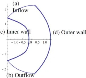
Geometry Let k be the streamline parameter, i.e. k= constant on each streamline. The streamlines corresponding to the two wall boundaries are k=kmax= 1.5 for the inner wall, and
k=kmin= 0.7 for the outer wall. Letq be the velocity magnitude. For each fixedk,kmin≤k≤
kmax, the variableqvaries betweenq0= 0.5andk. For eachq, define the speed of sounda, density ρ, pressurep, and a quantityJ by
a= r 1−γ−1 2 q 2; ρ=aγ−12 ; p= 1 γa 2γ γ−1; J = 1 a+ 1 3a3 + 1 5a5 − 1 2log 1 +a 1−a (16)
For each pair(q, k), set
x(q, k) = 1 2ρ 2 k2 − 1 q2 −J 2, y(q, k) =± 1 kρq r 1−q k 2 (17) Again,q0= 0.4,kmin= 0.7,kmax= 1.5, the four boundaries are (a) inflow,q=q0,kmin≤k≤kmax,
andy >0; (b) outflow,q=q0,kmin≤k≤kmax, andy <0; (c) inner wall,k=kmaxandq0≤q≤k; (d) outer wall,k=kmin. See Figure2.
Exact Solution The exact solution is given by (16) and (17). The flow is irrotational and isentropic. It reaches a supersonic speed of Mach number 1.5 at locationy= 0of the inner wall. Entropy should be a constant in the flow field.
Figure 2. Ringleb geometry; thick curves: walls; thin curves: inflow and outflow boundaries.
4.3. Problem C1.3. Flow over a NACA 0012 Airfoil
Overview This problem aims at testing high-order methods for the computation of external flow with a high-order curved boundary representation. Both inviscid and viscous, subsonic and transonic flow conditions will be simulated. The transonic problem will also test various methods’ shock capturing ability. The lift and drag coefficients will be computed, and compared with those obtained with low-order methods.
Governing Equations The governing equations are 2D Euler and Navier-Stokes with a constant ratio of specific heats of 1.4 and Prandtl number of 0.72. For the viscous flow problem, the viscosity is assumed a constant.
Flow Conditions Three different flow conditions are considered: (a) Subsonic inviscid flow withM∞= 0.5, and angle of attackα= 2o.
(b) Inviscid transonic flow withM∞= 0.8, andα= 1.25o.
(c) Subsonic viscous flow withM∞= 0.5, andα= 1, Reynolds number (based on the chord
length)Re= 5,000.
Geometry The geometry is a NACA 0012 airfoil, modified to close the trailing edge. The resulting analytical expression for the airfoil surface is
y=±0.6 0.2969√x−0.1260x−0.3516x2+ 0.2843x3−0.1036x4
The airfoil geometry is shown in Figure3.
Boundary Conditions Subsonic inflow and outflow on the far-field boundary. Slip wall for inviscid flow, or no slip adiabatic wall for viscous flow.
4.4. Problem C1.4. Laminar Boundary Layer on a Flat Plate
Overview This problem aims at testing high-order methods for viscous boundary layers, where highly clustered meshes are employed to resolve the steep velocity gradient. The drag coefficient will be computed and compared with that obtained with low-order methods.
Governing Equations The flow is governed by the 2D Navier-Stokes equations with a constant ratio of specific heats of 1.4 and Prandtl number of 0.72. The dynamic viscosity is also a constant.
Flow Conditions M∞= 0.5, angle of attackα= 0o. Reynolds number (based on the plate length)
ReL= 106.
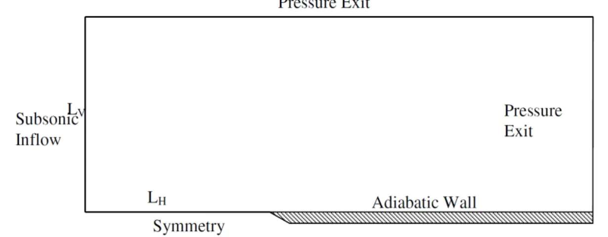
Geometry The plate lengthLis assumed 1. The computational domain has two other length scales
LH andLV, as shown in Figure4. Participants should assess the influence of these length scales to
the numerical results, and select large enough values that the numerical results are not affected by them.
Figure 4. Computational Domain for the Flat Plate Boundary Layer.
Boundary Conditions As depicted in Figure4
4.5. Problem C1.5. Radial Expansion Wave (2D or 3D)
Overview Boundary Conditions
Governing Equations The governing equation is the 2D or 3D Euler equations with a constant ratio of specific heats ofγ= 1.4.
Flow Conditions The initial condition is defined everywhere. The flow is cylindrically (2D) or spherically (3D) symmetric but computed on a Cartesian grid. The flow field is purely radial. The initial distribution of the radial velocityqis infinitely differentiable:
q(r,0) = 0, 0≤r < 1 2 1 γ 1 + tanh0.25−r−(r1−1)2 , 12 ≤r < 32 2 γ, r≥ 3 2
The Cartesian velocity components are related toqat any time and place by
u= x rq, v= y rq, w= z rq,
The initial distribution of the speed of sound a derives fromq(r,0):
a(r,0) = 1−γ−1 2 q(r,0).
Here the ratio of specific heats may be chosen by the user from the interval 1< γ <3, e.g. 7/5 (aero), 5/3 (astro), 2 (civil, atmospheric). For this workshop,γ= 7/5. The density initially equalsγ
in the origin and further follows from assuming uniform entropy
ρ(r,0) =γa2/(γ−1)
The initial values of any other flow quantity derive from the above equations and the perfect-gas law, e.g., pressure:
p= ρa
2
γ .
Because the flow is entirely determined by the initial values, these should be carefully discretized. For instance, if the numerical method is a finite-volume scheme that updates the cell- averages of the conserved flow quantities, these must be computed from the analytical initial values by a sufficiently accurate Gaussian quadrature. The same holds for the integrals needed to compute the weights of the basis functions in a Discontinuous Galerkin discretization. If superconvergence is anticipated, the order of accuracy of the Gaussian quadrature must be taken high enough so as not to obscure the truncation error of the scheme with an initialization error. At outflow the Mach number is 2, which means supersonic outflow normal to all domain boundaries, in both 2D and 3D.
Geometry The computational domain is a square (cube)[4,4]×[4,4](×[4,4]), uniformly divided into cells with∆x= ∆y(= ∆z) =h, wherehtakes the values 1/8 (grid 1), 1/16 (grid 2), 1/32 (grid 3), etc. The simulations should be run fromt= 0tot= 3. The largest wave speed appearing in the problem is3/γ, which may be helpful in setting the time step. However, tests should be performed to ensure that the time step is small enough (or the order of time integration is high enough) that temporal resolution has minimal effect on the results.
4.6. Problem C1.6. Vortex Transport by Uniform Flow
Overview This problem aims at testing a high-order method’s capability to preserve vorticity in an unsteady inviscid flow. Accurate transport of vortices at all speeds (including Mach number much less than 1) is very important for Large-Eddy and Detached-Eddy simulations, possibly the workhorse of future industrial CFD simulations, as well as for aeronautics/rotorcraft applications.
Governing Equations The governing equations are the unsteady (2D) Euler equations, with a constant ratio of specific heats ofγ= 1.4and gas constantRgas= 287.15J/kg.K.
Flow Conditions The domain is first initialized with a uniform flow of pressureP∞, temperature
T∞, a given Mach number (see Testing Conditions below), and a vortical movement of characteristic
radiusRand strengthβsuperimposed around the point at coordinates(Xc, Yc):
δu = −(U∞β) y−Yc R exp −r2 2 δv = (U∞β) x−Xc R exp −r2 2 δT = 1 2Cp (U∞β)2exp(−r2) u0 = U∞+δu v0 = δv where Cp = γ γ−1Rgas r = p (x−Xc)2+ (y−Yc)2 R U∞ = M∞pγRgasT∞.
Note,U∞is the speed of the unperturbed flow. The pressure, temperature and density are prescribed
such that the superimposed vortex is a steady solution of the stagnant (e.g. without uniform transport) flow situation:
T0 = T∞−δT ρ0 = ρ∞ T0 T∞ 1/(γ−1) ρ∞ = P∞ RgasT∞ Pressure is computed as P0 = ρ0RgasT0
The superimposed vortex should be transported without distortion by the flow. Thus, the initial flow solution can be used to assess the accuracy of the computational method (seeRequirementsbelow).
Geometry The computational domain is rectangular, with(x, y)∈[0, Lx]×[0, Ly].
Boundary Conditions Translational periodic boundary conditions are imposed for the left/right and top/bottom boundaries respectively.
Testing Conditions Assume that the computational domain dimensions (in meters) are Lx= 0.1, Ly = 0.1 and set Xc= 0.05[m], Y c= 0.05[m] (marking the center of the computational
domain),P∞= 105N/m2, andT∞= 300K.
Consider the following flow configurations:
1. “Slow vortex”:M∞= 0.05, β= 1/50, R= 0.005.
2. “Fast vortex”:M∞= 0.5, β= 1/5, R= 0.005.
Define the time-periodT asT =Lx/U∞ and perform a “long” simulation, where the solution is
advanced in time for 50 time periods. That is, simulate the vortex evolution in time for50T.
4.7. Problem C2.1. Unsteady Viscous Flow over Tandem Airfoils
Overview This problem aims to test the unsteady interaction of a vortex with a solid wall. Specifically, several cases are defined that address both unsteady pressure generation and viscous separation in a 2D framework by using a pair of airfoils. The geometry remains relatively simple and provides a test bed for several different types of analysis. In general, the time history of the lift coefficient on the aft airfoil will be used as a metric. Other quantities to assess would be the pressure distribution on the two airfoils and the total circulation in the problem obtained by integrating the vorticity throughout the domain.
Governing Equations The governing equations for this problem are the 2D compressible Navier-Stokes equations with a constant ratio of specific heats equal to1.4and a Prandtl number of0.72. Compressibility is not anticipated to be a significant player in these problems. Specific conditions will be provided with each subcase.
Flow Conditions Two different problems are defined. In each of these cases, the Mach number (M∞) is0.2, the angle of attack (α) is0◦, and the Reynolds number based on the chord of one of
the airfoils is104.
• Case A examines the evolution of the flow field from a prescribed initial solution that isC1. In this condition,dis the distance to the closest wall, which is often required for turbulence models. Density and pressure are initialized to their free-stream values.
v= (u, v) =M∞ rγp ∞ ρ∞ (cosα,sinα) 1, d > δ1 sin2πdδ 1 , d≤δ1 (18) withδ1= 0.05.
• Case B is closer to an impulsive start condition. Lets(r) = (r−(δ2,0))·(cosα,sinα)with δ1= 0.5. Density and pressure are again set to uniform free-stream values.
v= (u, v) =M∞ rγp ∞ ρ∞ (cosα,sinα) 1, s <−δ3 −sin2πsδ 3 , −δ3≤s≤0 0, s >0 (19) withδ3= 0.1.
Geometry The basic geometry for this case is two relatively positioned NACA0012 airfoils, which were described for problem C.1.3. The leading airfoil is rotated byδabout(0.25c,0)while the trailing airfoil is translated by(1 +dsep,−doff)c. For the present case, takeδ= 10◦,dsep= 0.5, anddoff= 0. The far field boundary can be determined such that the steady state lift coefficient of both airfoils varies by less than0.01counts.
Figure 5. Geometry for Tandem Airfoils.
4.8. Problem C2.2. Steady Turbulent Transonic flow over an Airfoil
Overview This problem aims at testing high-order methods for a two-dimensional turbulent flow under transonic conditions with weak shock-boundary layer interaction effects. The test case is the RAE2822 airfoil Case 9, for which an extensive experimental database exists [27]. The test case has also been investigated numerically by many authors using low order methods. It was also used in the European project ADIGMA (test case MTC5). The target quantities of interest are the lift and drag coefficients and the skin friction distribution at one free-stream condition, as described below.
Governing Equations The governing equation is the 2D Reynolds-averaged Navier-Stokes equations with a constant ratio of specific heats of1.4and Prandtl number of 0.71. The dynamic viscosity is also a constant. The choice of turbulence model is left up to the participants; recommended suggestions are 1) the Spalart-Allmaras model, and 2) the Wilcox k-ω model or EARSM.
Flow Conditions Only Case 9 is retained for this workshop. The original flow conditions in the wind tunnel experiment areM∞= 0.730, angle of attackα= 3.19◦, Reynolds number (based on the
reference chord) Re= 6.5·106. However, in order to take into account the wind tunnel corrections for comparison with experimental data the computations for the workshop have to be made with corrected flow conditions, namely Mach numberM∞= 0.734, angle of attackα= 2.79◦, with the
same Reynolds number. Laminar to turbulent transition is fixed at3%of the chord, on both pressure and suction side. No further wind tunnel effects are to be modeled.
Geometry Originally the geometry is defined with a set of points. These points are then used to define a high-order geometry, which is available online at the workshop web site.
Boundary Conditions Adiabatic no-slip wall on the airfoil surface, free-stream at the farfield (subsonic inflow / outflow). A sensitivity study must be performed to find a far field boundary location whose effect on the lift and drag coefficient is less than0.01counts, i.e.,10−6.
4.9. Problem C2.3. Analytical 3D Body of Revolution
Overview This problem defined in ADIGMA as test case BTC0 [23] is aimed at testing high-order methods for the computation of external flow with a high-order curved boundary representation in 3D. Inviscid, viscous (laminar) and turbulent flow conditions will be simulated.
Governing Equations The governing equations for inviscid and laminar flows are the 3D Euler and Navier-Stokes equations with a constant ratio of specific heats of 1.4 and Prandtl number of
0.72. For the laminar flow problem, the viscosity is assumed a constant.
Flow Conditions Inviscid: M∞ = 0.5 α = 1◦ , Laminar: M∞ = 0.5 α = 1◦ Re = 5,000 , Turbulent: M∞ = 0.5 α = 5◦ Re = 10·106
Geometry The geometry is a streamlined body based on a 10 percent thick airfoil with boundaries constructed by a surface of revolution. The airfoil is constructed by an elliptical leading edge and straight lines. Half model: y∈ 0,1001 : 16 x−1 4 2 + 400z2= 1, x∈ 0,13 z= 1 10√2(1−x), x∈ 1 3,1 , z >0 z=− 1 10√2(1−x), x∈ 1 3,1 , z <0 y > 1001 : 16 x−1 4 2 + 400z2+ y− 1 100 2 = 1, x∈ 0,13 200z2+ y− 1 100 2 −(1−x)2= 0, x∈ 1 3,1
Figure 6. 3D Body of Revolution.
Reference values
• Reference area:0.1(full model)
• Reference moment length:1.0 • Moment line: quarter chord
Boundary Conditions
• Far field boundary: Subsonic inflow and outflow
• Wing surface: no slip adiabatic wall
4.10. Problem C2.4. Laminar Flow around a Delta Wing
Overview This problem aims at predicting vortex dominated flows. A laminar flow at high angle of attack around a delta wing with a sharp leading edge and a blunt trailing edge is selected (see also [23]). As the flow passes the leading edge it rolls up and creates a vortex together with a secondary vortex. The vortex system remains over a long distance behind the wing. This problem also aims at testing high-order and adaptive methods for the computation of vortex dominated external flows. Note, that methods which show high-order on smooth solutions will show about 2nd order only on this test case because of reduced smoothness properties (e.g. at the sharp edges) of the flow solution. Finally, alsoh-adaptive, andhp-adaptive computations can be submitted for this test case.
Governing Equations The governing equation is the 3D Navier-Stokes equations with a constant ratio of specific heats of1.4and Prandtl number of0.72. The viscosity is assumed a constant.
Flow Conditions Subsonic viscous flow with M∞= 0.3, and α= 12.5◦, Reynolds number
(based on the mean cord length)Re = 4,000.
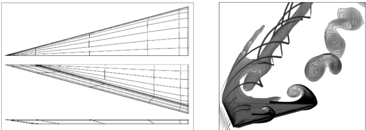
Geometry The geometry is a delta wing with a sloped and sharp leading edge and a blunt trailing edge. A precise definition of the geometry can be found in [28,29]. Fig.7shows the top, bottom and side views of a half model of this wing.
Figure 7. Left: Top, bottom and side view of the half model of the delta wing. The grid has been provided by NLR within the ADIGMA project. Right: Streamlines and Mach number isosurfaces of the flow solution over the left half of the wing and Mach number slices over the right half. The figures are taken from [30].
Reference values
• Reference area:0.133974596(half model)
• Reference moment length:1.0 • Moment line: quarter chord
Boundary Conditions
• Far field boundary: subsonic inflow and outflow
• Wing surface: no slip isothermal wall withTwall=T∞.
4.11. Problem C3.1. Turbulent Flow over a 2D Multi-Element Airfoil
Overview This problem aims at testing high-order methods for a two-dimensional turbulent flow with a complex configuration. It has been investigated previously with low order methods as part of a NASA Langley workshop. The target quantities of interest are the lift and drag coefficients at one free-stream condition, as described below.
Governing Equations The governing equation is the 2D Reynolds-averaged Navier-Stokes equations with a constant ratio of specific heats of1.4and Prandtl number of 0.71. The dynamic viscosity is also a constant. The choice of turbulence model is left up to the participants; recommended suggestions are 1) the Spalart-Allmaras model, and 2) the Wilcox k-ωmodel.
Flow Conditions Mach numberM∞= 0.2, angle of attackα= 16◦, Reynolds number (based on
the reference chord)Re = 9·106. The boundary layer is assumed fully turbulent and no wind tunnel effects are to be modeled.
Geometry The multi-element airfoil geometry is shown in the following figure. Originally the geometry is defined with a set of points. These points are then used to define a high-order geometry, which is available online at the workshop web site. The reference chord length is0.5588m.
Figure 8. MDA 30P-30N multi-element airfoil geometry.
Boundary Conditions Adiabatic no-slip wall on the airfoil surface, free-stream at the farfield.
4.12. Problem C3.2. Turbulent Flow over the DPW III Wing Alone Case
Overview This problem aims at testing high-order methods for a three-dimensional wing case with turbulent boundary layers at transonic conditions. This problem has been investigated previously with low-order methods as part of the AIAA drag prediction workshop, [31] (see DPW-W1). The target quantity of interest is the drag coefficient at one free-stream condition, as described below.
Governing Equations The governing equation is the 3D Reynolds-averaged Navier-Stokes equations with a constant ratio of specific heats of1.4and Prandtl number of 0.71. The dynamic viscosity is also a constant. The choice of turbulence model is left up to the participants; recommended suggestions are 1) the Spalart-Allmaras model, and 2) the Wilcox k-ωmodel.
Flow Conditions Mach numberM∞= 0.76, angle of attackα= 0.5◦, Reynolds number (based
on the reference chord)Recref = 5·106. The boundary layer is assumed fully turbulent and no wind tunnel effects are to be modeled.
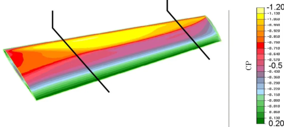
Geometry The wing geometry, illustrated in Figure 9 with pressure contours, is a simple trapezoidal planform with modern supercritical airfoils. The precise geometry definition is available online athttp://aaac.larc.nasa.gov/tsab/cfdlarc/aiaa-dpw/Workshop3/.
Reference values
• Planform area:Sref= 290,322mm2= 450in2
• Chord:cref= 197.556mm= 7.778in
• Span:b= 1,524mm= 60in
Boundary Conditions Adiabatic no-slip wall on the wing, symmetry at the wing root, and free-stream at the farfield.
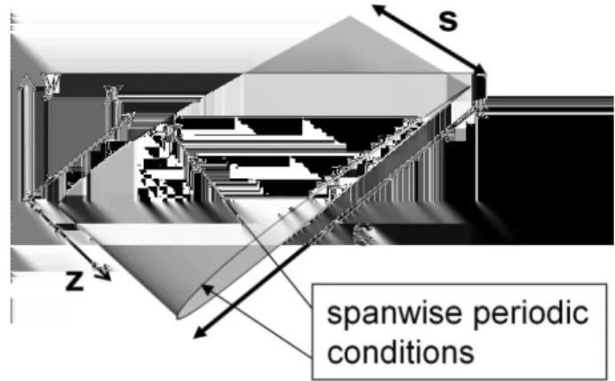
4.13. Problem C3.3. Transitional Flow over a SD7003 Wing
Overview This test case aims at characterizing the accuracy and performance of high-order solvers for the prediction of complex unsteady transitional flows over a wing section under low Reynolds number conditions. Of particular interest is the evaluation of so-called Implicit Large-Eddy Simulation (or ILES) approaches for handling, in a seamless fashion, the mixed laminar, transitional, and turbulent flow regions encountered in these low-Re applications. The unsteady flow is characterized by laminar separation, the formation of a transitional shear layer followed by turbulent reattachment. In a time-averaged sense, a laminar separation bubble (LSB) is formed over the airfoil.
Governing Equations The governing equations are the full 3D compressible Navier-Stokes equations with a constant ratio of specific heats of 1.4 and Prandtl number of 0.72. Solutions obtained employing the fully incompressible Navier-Stokes equations are also desired. Given the low value of Reynolds number being considered, emphasis is placed on ILES approaches; however, methodologies which incorporate dynamic sub-grid-scale (SGS) models are also of interest.
Flow Conditions
• Mach numberM = 0.1.
• Reynolds number based on wing chord,Rec = 60,000. • Angle of attack:
– Case 1.α= 4◦, which corresponds to a relatively long LSB
– Case 2.α= 8◦, which corresponds to a shorter LSB
Geometry The wing section is based on the Selig SD7003 airfoil profile shown in Fig.7. This airfoil which was originally designed for low-Reynolds number operation (Rec ∼105), has a
maximum thickness of8.5%and a maximum camber of1.45% atx/c= 0.35. The original sharp trailing edge has been rounded with a very small circular arc of radius r/c∼0.0004in order to facilitate the use on an O-mesh topology. The precise profile of the geometry is provided in [32]. The flow is considered to be homogeneous in the spanwise direction with periodic boundary conditions being imposed over a widths/c= 0.2.
Figure 10. The SD 7003 wing.
• Far field boundary: subsonic inflow and outflow. This boundary should be located very far from the wing at a distance of∼100chords
• Airfoil surface: no slip isothermal wall conditions withTwall/Tinf= 1.002.
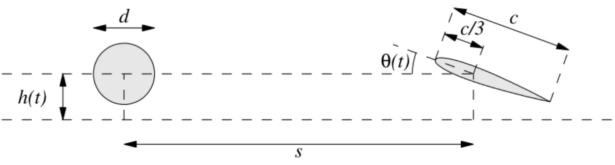
4.14. Problem C3.4. Heaving and Pitching Airfoil in Wake
Overview This problem aims at testing the accuracy and performance of high-order flow solvers for problems with deforming domains. An oscillating cylinder produces vortices that interact with an airfoil performing a typical flapping motion. The time histories of the drag coefficient on both the cylinder and on the airfoil are used as metrics, and two test cases corresponding to different stream-wise positions of the airfoil are studied.
Governing Equations The governing equations for this problem are the 2D compressible Navier-Stokes equations with a constant ratio of specific heats equal to1.4and a Prandtl number of0.72.
Flow Conditions The free-stream has the magnitudeU∞= 1, a Mach number (M∞) of0.2, and
an angle of attack (α) of0degrees. The Reynolds number based on the chord of the airfoil is1,000
(or, equivalently,500based on the diameter of the cylinder).
Geometry The geometry consists of a cylinder of diameterd= 0.5centered at the origin, and a NACA0012 airfoil with chord length c= 1 positioned downstream from the cylinder. The airfoil geometry is given by the modification of thex4-coefficient to give zero trailing edge thickness, as described for case C1.3. The center of the cylinder and the1/3-chord of the airfoil are separated by a distances. Both bodies are heaving in an oscillating motionh(t) =Asinωt, whereA= 0.25and
ω= 2π·0.4(in the workshop, the angular velocityω= 2π·0.2was used). In addition, the airfoil is pitching about its1/3-chord by an angleθ(t) =asin(ωt+ϕ), where the amplitudea=π/6and the phase shiftϕ=π/2.
h(t)
θ
(t)
s
d
c
c/3
Figure 11. The heaving and pitching airfoil problem.
4.15. Problem C3.5 Direct Numerical Simulation of the Taylor-Green Vortex atRe= 1600 Overview This problem is aimed at testing the accuracy and the performance of high-order methods on the direct numerical simulation of transitional flows. The test case concerns a three-dimensional periodic and transitional flow defined by a simple initial condition: the Taylor-Green vortex. The initial flow field is given by
u = V0 sin x L cosy L cosz L , v = −V0 cos x L siny L cosz L , w = 0, p = p0+ ρ0V02 16 cos 2x L + cos 2y L cos 2z L + 2 .
This flow transitions to turbulence with the creation of small scales, followed by a decay phase similar to homogeneous isotropic turbulence (see Figure12).
Figure 12. Illustration of Taylor-Green vortex att= 0(left) and attfinal= 20tc(right): iso-surfaces of the
Governing Equations The flow is governed by the 3D incompressible Navier-Stokes, or alternatively, the 3D compressible Navier-Stokes equations at low Mach number. In both cases, the physical parameters of the model are taken to be constant.
Flow Conditions The Reynolds number of the flow is defined as Re=ρ0V0L
µ and is equal to 1600. If modeling compressible flow, the fluid is assumed a perfect gas with γ=cp/cv= 1.4,
Prandtl numberP r=µ cp
κ = 0.71, and zero bulk viscosity:µv= 0. In addition, the Mach number
is taken as M0= Vc00 = 0.10, where c0 is the speed of sound corresponding to the temperature T0=R ρp0
0, and the initial temperature field is assumed uniform:T =T0; so that the initial density field is taken asρ= R Tp
0.
The physical duration of the computation is based on the characteristic convective timetc=VL
0 and is set to tfinal= 20tc. As the maximum of the dissipation (and thus the smallest turbulent
structures) occurs att≈8tc, participants can also decide to only compute the flow up tot= 10tc
and report solely on those results.
Geometry The flow is computed within a periodic cube defined as−πL≤x, y, z≤πL.
Grids Participants were encouraged to perform a grid or order convergence study if feasible. At least one computation was required on a baseline resolution of approximately2563DOFs (degrees of freedom):e.g., for DGM using 4th order polynomial interpolants, this corresponds643elements.
Mandatory results Each participant was requested to provide the following data:
• The temporal evolution of the kinetic energy integrated on the domainΩ:
Ek= 1 ρ0Ω Z Ω ρv·v 2 dΩ.
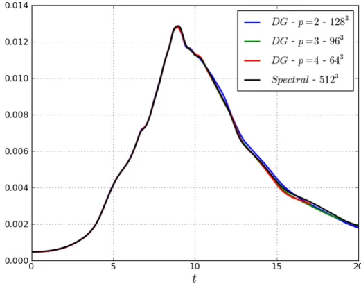
• The temporal evolution of the kinetic energy dissipation rate:=−dEk
dt . The typical evolution
of the dissipation rate is illustrated in Figure13.
• The temporal evolution of the enstrophy integrated on the domainΩ:
E= 1 ρ0Ω Z Ω ρω·ω 2 dΩ.
This is indeed an important diagnostic asis also exactly equal to2ρµ
0E for incompressible flow and approximately for compressible flow at low Mach number.
• The vorticity norm on the periodic faceLx =−πat timett
c = 8for comparison to the reference
results. An illustration is given in Figure14. For brevity, the results of this comparison are not treated in this paper.
Reference data The results are compared to a reference incompressible flow solution. This solution was obtained using a de-aliased pseudo-spectral code (developed at Universit´e catholique de Louvain, UCL) for which, spatially, neither numerical dissipation nor numerical dispersion errors occur; the time-integration is performed using a low-storage 3-steps Runge-Kutta scheme [33], with
Figure 13. Evolution of the dimensionless energy dissipation rate as a function of the dimensionless time: results of pseudo-spectral code and of variants of a DG code.
Figure 14. Iso-contours of the dimensionless vorticity norm, VL0|ω|= 1,5,10,20,30, on a subset of the periodic face xL=−πat time tt
c = 8. Comparison between the results obtained using the pseudo-spectral
code (black) and those obtained using a DG code withp= 3and on a963mesh (red).
a dimensionless time step of1.0 10−3. These results have been grid-converged on a5123grid (a grid convergence study for a spectral discretization has also been done by van Rees et al. in[34]); this
means that all Fourier modes up to the 256th harmonic with respect to the domain length have been captured exactly (apart from the time integration error of the Runge-Kutta scheme). However, an adequate resolution is already obtained at2563, which is the baseline requirements for the test case.
5. CURRENT STATUS – SAMPLE RESULTS
In this section we present a subset of the results analyzed and reviewed in the course of the workshop. Not all cases are included, but the ones chosen form a representative sampling that supports several conclusions. In presenting the results we will make use of several acronyms, which are defined in TableI.
Table I. Acronyms used in the results presentation.
Acronym Definition
FVM Finite-volume method DG Discontinuous Galerkin
CPR Correction procedure via reconstruction SEM Spectral-element method
RK4 Fourth-order Runge-Kutta
RDG Reconstructed discontinuous Galerkin
DRP Dispersion relation preserving (finite difference)
5.1. Inviscid flow through a channel with a smooth bump
This is an example of a smooth flow for which high-order schemes are expected to perform very well compared to low-order schemes. Ten groups submitted full or partial results for this case, using a variety of methods, as listed in TableII. With the exception of the MIT group, all participants used a sequence of nested uniformly-refined meshes. The MIT group generated output-based optimized meshes at several fixed degrees of freedom.
Table II. Inviscid flow through a channel with a smooth bump: summary of participants.
Group Affiliation Authors Method
UTenn Univ. of Tennessee at Chattanooga Wang, Anderson, Erwin DG
UM Univ. of Michigan Khosravi, Fidkowski DG
UBC Univ. of British Columbia Ollivier-Gooch High-order FV MIT Massachusetts Inst. of Technology Yano, Darmofal DG
ONERA ONERA S. G´erald DG
Twente Univs. of Twente and Edinburgh van der Weide and Sv¨ard Finite difference
ISU Iowa State Univ. Li, Wang CPR-DG
UC Univ. of Cincinnati and AFRL Galbraith, Orkwis, Benek DG
Glenn NASA Glenn Huynh DG
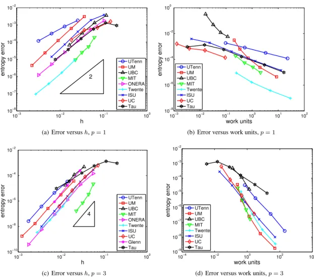
A subset of the results for entropy error convergence is presented in Figure15. Shown are the data points for all the groups at approximation orderp= 1andp= 3, i.e. formally second and fourth order, respectively. Although additional orders were compared in the workshop, only these two are shown here for brevity;p= 1was chosen because it is expected to be similar to traditional second-order schemes andp= 3was chosen as a representative high-order result. Results from a second-order reconstructed finite-volume result, obtained using the Tau code, are shown for reference on
all of the plots. We immediately see that high order (p= 3) is, across the board, more efficient in degrees of freedom thanp= 1. Among the participants, the spread in error versushis smaller for
p= 3compared top= 1. The spread in work units is large for both orders shown, indicating that implementation and coding vary significantly.
10−3 10−2 10−1 100 10−8 10−7 10−6 10−5 10−4 10−3 10−2 2 h entropy error UTenn UM UBC MIT ONERA Twente ISU UC Tau
(a) Error versush,p= 1
10−3 10−2 10−1 100 101 102 10−8 10−6 10−4 10−2 100 work units entropy error UTenn UM UBC MIT Twente ISU UC Tau
(b) Error versus work units,p= 1
10−3 10−2 10−1 100 10−10 10−8 10−6 10−4 10−2 4 h entropy error UTenn UM UBC MIT ONERA Twente ISU UC Glenn Tau (c) Error versush,p= 3 10−4 10−2 100 102 104 10−9 10−8 10−7 10−6 10−5 10−4 10−3 10−2 work units entropy error UTenn UM UBC MIT Twente ISU UC Tau
(d) Error versus work units,p= 3
Figure 15. Inviscid flow through a channel with a smooth bump: entropy error norm versus mesh size and work units, shown for two different approximation orders.
On average,p= 1results are similar to the reference finite-volume solution. On the other hand,
p= 3results from nearly all of the participants outperform the reference FVM solution in terms of degrees of freedom and work units. Furthermore, as expected, the ideal asymptotic convergence rates are attained for this smooth problem.
5.2. Flow over the NACA 0012 airfoil, inviscid and viscous, subsonic and transonic
In this section we present results from all sub-cases of Case 1.3: these are (a) inviscid subsonic, (b) transonic flow, and (c) viscous subsonic. Participants that submitted results for this case are listed in TableIII. We note again that the MIT group generated output-based optimized meshes at fixed degrees of freedom. The University of Wyoming group (UW) used anhp-refinement strategy, while
all other participants used sets of uniformly-refined meshes. The MIT and UW groups, as well as the University of British Columbia group (UBC) used triangular meshes, while the remaining participants used a quadrilateral mesh topology. The DLR and UM groups, as well as the Iowa State University group (ISU) used the quadrilateral meshes provided to participants via the conference website, while the remaining groups generated meshes independently.
Table III. Flow over the NACA 0012 airfoil: summary of participants.
Group Affiliation Authors Method
MIT Massachusetts Inst. of Technology Yano, Darmofal DG
UM Univ. of Michigan Fidkowski DG
UBC Univ. of British Columbia Ollivier-Gooch High-order FV
DLR DLR Hartmann DG
Twente Univs. of Twente and Edinburgh van der Weide and Sv¨ard Finite difference
ISU Iowa State Univ. Zhou, Wang CPR-DG
UW Univ. of Wyoming Burgess, Mavriplis DG
It should be appreciated that no exact analytical solutions were used to measure the error for this test case. Instead, each participant provided a convergence study based on a reference solution that he or she generated at higher resolution (finer grid, and/or using polynomials of higher degree). However, there were no common standards by which the reference solution was generated, and furthermore, not all participants provided the details of their individual approach. The reference solutions that were used by the participants showed a scatter on a level similar to that approached by the errors in mesh refinement. Consequently, results for this test case should be interpreted as qualitative in nature.
We show a representative subset of the results submitted by the participants. For both the subsonic and the transonic test cases we compare results forp= 3with results forp= 1, obtained with the same respective method. Furthermore, we again compare the results to those from a second-order reconstructed finite-volume method (FVM), computed by the DLR Tau code.
Results for the subcritical case are shown in Figures16and17. High order (p= 3) is observed to be more efficient in degrees of freedom and work units than low order (p= 1). Thep= 1results, on average, are similar to reference FVM solution, while thep= 3results, for almost all simulations, outperform the reference FVM solution in terms of degrees of freedom and work units. This is true even for moderate levels of error. The spread in error versushis smaller for p= 3compared to
p= 1, while the spread in work units is fairly large for both orders. It should be noted that not all participants have optimized their solvers with respect to runtime. Therefore a somewhat larger scatter in work units is not surprising.
Asymptotic high-order convergence rates are not attained with uniform refinement at p= 3
due to a singularity at the trailing edge of the airfoil. The highest convergence rates, at least for drag, are observed with the fixed-degrees-of-freedom, output-based optimization strategy employed by the MIT group. This strategy is effectively able to isolate the trailing-edge singularity with appropriately-small elements, in contrast to uniform refinement of a fixed starting mesh. Note that the results from the DLR group and the UM group are very similar, when plotted againsth, as these two groups use the same discretization method (DG), and furthermore both groups used the meshes provided by the conference organizers.
10−3 10−2 10−1 10−5 10−4 10−3 10−2 10−1 100 h
drag coefficient error
2 MIT UM UBC DLR ISU Tau 10−4 10−2 100 102 104 10−5 10−4 10−3 10−2 10−1 100 work units
drag coefficient error
MIT UM DLR ISU Tau 10−3 10−2 10−1 10−4 10−3 10−2 10−1 h
lift coefficient error
2 MIT UM DLR ISU Tau 10−4 10−2 100 102 104 10−4 10−3 10−2 10−1 work units
lift coefficient error MIT
UM DLR ISU Tau
Figure 16. Inviscid subcritical flow over a NACA 0012 airfoil: lift and drag coefficient error convergence for
p= 1.
Results for the transonic case are shown in Figures18forp= 1, and Figure19 forp= 2. The plots show the reference FVM solution (TAU), a uniform refinement study (UM), and two adaptive studies (MIT, UW). It should be noted that the UW group, who contributed one of the adaptive solutions, actually performedhpadaptation using polynomial degrees ofp= 1throughp= 4. They provided one convergence study, so that the same results are shown in Figure18and Figure19. For the transonic case, the benefit of high order (p= 2in this case due to a larger data set submitted for
p= 2) overp= 1is not as great as for smooth problems. However, in generalp= 2does not fare worse thanp= 1in terms of degrees of freedom or even work units. Adaptive refinement generally performs better than uniform refinement, as expected, although convergence histories are not as regular as for smooth problems.
Results for the viscous case are shown in Figures 20 and 21. We note that the University of Wyoming group (UW) again submitted a result using an hp-refinement strategy. In addition, the residual convergence criterion for this case was relaxed from ten to eight orders of magnitude. The plots again include a reference FVM solution generated by the Tau code. In terms of both degrees of freedom and work units, most of thep= 1submissions are comparable to the reference FVM solution. Forp= 3, the submitted results show generally better performance than the FVM solution, especially when high accuracy is required.
10−3 10−2 10−1 10−8 10−7 10−6 10−5 10−4 10−3 10−2 10−1 h
drag coefficient error
4 MIT UM UBC DLR Twente ISU Tau 10−1 100 101 102 103 10−8 10−7 10−6 10−5 10−4 10−3 10−2 10−1 work units
drag coefficient error
MIT UM DLR Twente ISU Tau 10−3 10−2 10−1 10−6 10−5 10−4 10−3 10−2 10−1 h
lift coefficient error
4 MIT UM DLR Twente ISU Tau 10−1 100 101 102 103 10−6 10−5 10−4 10−3 10−2 10−1 work units
lift coefficient error
MIT UM DLR Twente ISU Tau
Figure 17. Inviscid subcritical flow over a NACA 0012 airfoil: lift and drag coefficient error convergence for
p= 3.
5.3. Vortex transport by uniform flow
This unsteady case, the last of the “easy” set, is relevant to various unsteady flows involving vortex propagation and resolution. The participants are listed in TableIV. We note that only DG results were submitted.
Table IV. Vortex transport by uniform flow: summary of participants.
Group Affiliation Authors Method
ISU Iowa State Univ. Li, Wang CPR-DG
UM Univ. of Michigan Fidkowski DG
Bergamo Univ. of Bergamo Bassi DG
JSU Jackson State Univ. Tu, Pang, Xiang DG
A subset of the submitted results is shown in Figure22. For comparison, a result using the second-order accurate STAR-CD code from CD-Adapco is shown and labeled as “Star”. High second-order in both space and time are important for observing optimal rates in solution convergence, as measured by the velocity error norm at the final time. We see that high-order results,p= 3, significantly outperform the low-order,p= 1, results in this case.
10−3 10−2 10−1 10−5 10−4 10−3 10−2 10−1 h
drag coefficient error
MIT UM UW Tau 10−1 100 101 102 103 104 10−5 10−4 10−3 10−2 10−1 work units
drag coefficient error
MIT UM UW Tau 10−3 10−2 10−1 10−8 10−6 10−4 10−2 100 h
lift coefficient error
MIT UM UW Tau 10−1 100 101 102 103 104 10−8 10−6 10−4 10−2 100 work units
lift coefficient error
MIT UM UW Tau
Figure 18. Transonic flow over a NACA 0012 airfoil: lift and drag coefficient convergence forp= 1.
5.4. Turbulent flow over an RAE airfoil
Three groups submitted results to this moderately-difficult case, which involved simulation of a Reynolds-averaged boundary layer and a transonic shock. A summary of the participants is given in TableV. Two of the groups used the Spalart-Allmaras (SA) turbulence model. The Bergamo group submitted two data sets, one with the explicit algebraic Reynolds-Stress model (EARSM), and one with the Wilcoxk−ωmodel. The MIT group submitted results using adaptive mesh optimization at fixed degrees of freedom, while the other groups submitted uniform-refinement results. All groups used discontinuous Galerkin for the discretization.
Table V. Turbulent flow over an RAE airfoil: summary of participants.
Group Affiliation Authors Method/Turbulence model
MIT Massachusetts Inst. of Technology Yano, Darmofal DG/SA
UM Univ. of Michigan Fidkowski DG/SA
Bergamo Univ. of Bergamo Bassi DG/EARSM &k−ω
The results for drag and lift coefficient are shown in Figure 23. The provided results show a large spread among the groups and virtually no improvement from high-order under uniform mesh refinement. Part of the spread in the uniform refinement results may be attributed to an inadequate wake alignment in the initial mesh. In this case, given the relative complexity of the flow, in particular the use of a Reynolds-averaged Navier-Stokes turbulence model, and the difficulty of
10−3 10−2 10−1 10−6 10−5 10−4 10−3 10−2 10−1 h
drag coefficient error
MIT UM UW Tau 10−1 100 101 102 103 104 10−6 10−5 10−4 10−3 10−2 10−1 work units
drag coefficient error MIT UM UW Tau 10−3 10−2 10−1 10−8 10−6 10−4 10−2 100 h
lift coefficient error
MIT UM UW Tau 10−1 100 101 102 103 104 10−8 10−6 10−4 10−2 100 work units
lift coefficient error
MIT UM UW Tau
Figure 19. Transonic flow over a NACA 0012 airfoil: lift and drag coefficient convergence forp= 2.
making an a priori initial mesh, adaptive mesh optimization is markedly superior. The other cause for spread in the results may be due to choice of turbulence model, as three different turbulence models were used by the participants.
5.5. Delta wing at low Reynolds number
The participants for this case are listed in TableVI. We note that only DG methods were submitted.
Table VI. Delta wing at low Reynolds number: summary of participants.
Group Affiliation Authors Method
DLR DLR Hartmann DG
UM Univ. of Michigan Fidkowski DG
Bergamo Univ. of Bergamo Bassi DG
UTenn Univ. of Tennessee at Chattanooga Wang, Anderson, Erwin DG
The results are shown in Figure24. High order shows some benefit in degrees of freedom, but in terms of work units, high order is comparable to low order. The singularity at the leading edge of the delta wing precludes high-order convergence rates and likely masks the benefit of high order with uniform mesh refinement. Some of the spread in the results can be ascribed to different mesh sequences used by the different groups (e.g. UTenn was not same as the others) and to different approximation spaces (e.g. Bergamo used a full-order space instead of a tensor product space). The
10−3 10−2 10−1 10−6 10−5 10−4 10−3 10−2 10−1 100 h
drag coefficient error
3 2 MIT UM DLR UW UW hp ISU Tau 10−2 100 102 104 106 10−6 10−5 10−4 10−3 10−2 10−1 100 work units
drag coefficient error
MIT UM DLR UW UW hp ISU Tau 10−3 10−2 10−1 10−5 10−4 10−3 10−2 10−1 100 h lift coefficient error 3
2 MIT UM DLR UW UW hp ISU Tau 10−2 100 102 104 106 10−5 10−4 10−3 10−2 10−1 100 work units
lift coefficient error
MIT UM DLR UW UW hp ISU Tau
Figure 20. Viscous flow over a NACA 0012 airfoil: lift and drag coefficient convergence forp= 1.
results of UM and DLR are almost identical in terms of accuracy over degrees of freedom due to the same numerical schemes used (BR2 scheme on a tensor product space), representing a perfect cross-code verification, while there are large differences in the work units required due to different solver strategies used.
5.6. Direct numerical simulation of the Taylor-Green vortex atRe= 1600
Starting out from a simple analytic initial solution, the transition of the Taylor-Green vortex at
Re= 1600 generates very complex three-dimensional (anisotropic) turbulent flow features. The transition is sufficiently robust such that it is not initiated by truncation errors. Therefore a detailed temporal comparison of the obtained solutions is possible.
The convergence analysis is based on the kinetic energy dissipation rate. A “grid” converged reference computation has been obtained using a incompressible pseudo-spectral method. The resolved spectrum contained up to the 256th spatial harmonic based on the width of the
computational domain (ie.5123 degrees of freedom (dof)per variable). Participants were required to perform at least one computation containing an equivalent resolution of 2563 subdivisions of the domain; based on a convergence study with the pseudo-spectral computations, this value seems to correspond to the Nyquist criterion based on the relevant spatial scales for this test case.
10−3 10−2 10−1 10−8 10−7 10−6 10−5 10−4 10−3 10−2 10−1 h
drag coefficient error
4 MIT UM DLR UW hp ISU Tau 10−2 100 102 104 106 10−8 10−7 10−6 10−5 10−4 10−3 10−2 10−1 work units
drag coefficient error
MIT UM DLR UW hp ISU Tau 10−3 10−2 10−1 10−7 10−6 10−5 10−4 10−3 10−2 10−1 100 h
lift coefficient error
4 MIT UM DLR UW hp ISU Tau 10−2 100 102 104 106 10−7 10−6 10−5 10−4 10−3 10−2 10−1 100 work units
lift coefficient error
MIT UM DLR UW hp ISU Tau
Figure 21. Viscous flow over a NACA 0012 airfoil: lift and drag coefficient convergence forp= 3.
10−3 10−2 10−1 10−5 10−4 10−3 10−2 10−1 h velocity error ISU, p=1 ISU, p=3 UM, p=1 UM, p=3 Bergamo, p=3 JSU, p=3 Star 101 102 103 104 105 106 10−5 10−4 10−3 10−2 10−1 work units velocity error ISU, p=1 ISU, p=3 UM, p=1 UM, p=3 Bergamo, p=3 JSU, p=3 Star
Figure 22. Vortex transport by uniform flow: convergence of velocity error withhand work units.
Compressible codes were required to run at an equivalent Mach number, corresponding to the reference velocity, of 0.1 to avoid (important) compressibility effects.
Two errors with respect to the reference results were defined. The first concerns the time derivative of the computed kinetic energy, whilst the second concerns the error on the theoretical dissipation rate, based on the integral of the enstrophy. A third error is defined as the difference between the