Lappeenranta-Lahti University of Technology LUT School of Engineering Science Degree Programme in Computational Engineering.

Degree Programme in Computational Engineering

Mikko Majamaa

GPGPU in System Simulations

Bachelor’s Thesis 2020

Supervisors: Arto Kaarna, Associate Professor Janne Kurjenniemi, Ph.D.

TIIVISTELM ¨A

Lappeenrannan-Lahden teknillinen yliopisto LUT School of Engineering Science

Laskennallisen tekniikan koulutusohjelma Mikko Majamaa

GPGPU in System Simulations

Kandidaatinty¨o 2020

30 sivua, 4 kuvaa, 5 taulukkoa, 2 liitett¨a Ohjaajat: Arto Kaarna, Tutkijaopettaja

Janne Kurjenniemi, Ph.D.

Avainsanat: GPGPU; systeemisimulaatio; CUDA; satelliitti; tietoverkko;

Systeemisimulointi voi olla laskennallisesti raskas teht¨av¨a. Grafiikkaprosessorin (GPU) avus-tuksella yleisess¨a laskennassa, voidaan hyv¨aksik¨aytt¨a¨a GPU:iden massiivista rinnakkaistet-tavuutta simulointiaikojen lyhent¨amiseksi. T¨am¨an kandidaatinty¨on tavoitteena on kirjal-lisuuskatsauksen avulla saavuttaa perustiet¨amys grafiikkaprosessoreilla teht¨av¨ast¨a yleises-t¨a laskennasta (GPGPU). Lis¨aksi tavoitteena on soveltaa saavutettu perustieyleises-t¨amys k¨ayyleises-t¨an- k¨ayt¨an-t¨o¨on toteuttamalla GPGPU:n k¨aytt¨o¨a Python-pohjaiseen satelliittiverkkosimulaattoriin. Tulokset osoittavat, ett¨a GPGPU:n k¨ayt¨oll¨a systeemisimuloinneissa on suuri potentiaali - sen k¨ayt¨oll¨a saavutettiin 16.0-kertainen kokonaisnopeutus ja 45.1-kertainen nopeutus linkkibud-jettilaskelmissa per¨att¨aiseen ajoon perustuvaan toteutukseen verrattuna.

Lappeenranta-Lahti University of Technology LUT School of Engineering Science

Degree Programme in Computational Engineering Mikko Majamaa

GPGPU in System Simulations

Bachelor’s thesis 2020

30 pages, 4 figures, 5 tables, 2 appendices Supervisors: Arto Kaarna, Associate Professor

Janne Kurjenniemi, Ph.D.

Keywords: GPGPU; system simulation; CUDA; satellite; network

Simulating systems can be computationally an expensive task. With the aid of graphics processing unit (GPU) in general-purpose computing one can execute programs exploiting GPU’s massive parallelism to reduce throughput time in simulations. The objective of this thesis is in literature review to achieve general knowledge on general-purpose computing on graphics processing units (GPGPU). Further objective is to implement usage of it into a Python-based satellite network simulator.

Results show that there is a great potential in using GPGPU in system simulations - a maxi-mum overall speed-up of 16.0x, as well as a speed-up of 45.1x in link budget computations were achieved compared to a sequential implementation.

FOREWORD

This bachelor’s thesis was carried out with a subject provided by Magister Solutions Ltd. I appreciate the company for providing me with such an interesting subject. Also, I want to thank my supervisor Arto Kaarna from LUT and Janne Kurjenniemi from the company, as well as my other co-workers too, for all the generous help I have received.

Mikko Majamaa Mikko Majamaa

1 INTRODUCTION 9

1.1 Background . . . 9

1.2 Objectives . . . 9

1.3 Structure of the report . . . 10

2 LITERATURE REVIEW 11 2.1 GPGPU . . . 11

2.2 GPGPU hardware and software environments . . . 13

2.3 GPGPU applications . . . 14

2.4 GPGPU in system simulations . . . 16

2.5 Summary . . . 17

3 SOFTWARE AND DATA 18 3.1 Satellite network simulator . . . 18

3.2 Numba . . . 18

4 EXPERIMENTS AND RESULTS 20 4.1 Implementation . . . 20

4.2 Comparison . . . 20

4.3 Profiling the simulator . . . 22

4.4 Use of shared memory . . . 23

5 DISCUSSION 26

6 CONCLUSION 27

APPENDICES

Appendix 1: Link budget computations

AES Advanced Encryption Standard API Application Programming Interface ASIC Application-Specific Integrated Circuit CDF Cumulative Distribution Function Cg C for graphics

CNN Convolutional Neural Network CPU Central Processing Unit

CTM Close to Metal

CUDA Compute Unified Device Architecture DCE Direct Code Execution

DE Differential Equation

FPGA Field-Programmable Gate Array

GPGPU General-Purpose Computing on Graphics Processing Units GPU Graphics Processing Unit

JIT Just-In-Time LEO Low Earth Orbit ns-3 Network Simulator 3

RRM Radio Resource Management SIMD Single Instruction, Multiple Data SNR Signal-to-Noise Ratio

SPMD Single Program, Multiple Data UAV Unmanned Aerial Vehicle UT User Terminal

SYMBOLS

C_jk Link budget

n_{SAT S} Number of satellites nt Number of parallel threads n_{U T S} Number of user terminals

s Portion of a program that is sequential t₁ Run time of a sequential program

1

INTRODUCTION

The objective of this thesis is to study GPGPU and with the achieved knowledge to imple-ment it’s usage into a Magister Solutions Ltd’s Python-based satellite network simulator.

1.1

Background

Usage of simulation as a part of the system development can improve the results of outcome, save expenses and even improve safety. According to White and Ingalls [1] the purpose of simulations is to provide a model and based on that model to predict the behaviour of a system of interest. They divide simulations into two different groups: human-in-the-loop simulations, used by e.g. firemen to simulate a housefire for training purposes, and analysis and design of processes and products, used by e.g. engineers and researches in their work. As moving forward the focus of this thesis will be more on system simulations, wireless network simulations and satellite network simulations. In wireless networks the devices connected to the network are connected through radio waves [2]. By simulating networks one can test new scenarios, simulate the effects of network traffic or different protocols to the network performance and visualize the network performance and different events happening in the simulation [3].

Traditionally network simulators have been based on sequential execution [3]. However, compared to sequential execution more efficient way to execute programs is to design them such that they can be parallelized. Parallelized programs can then be executed using mul-tiple cores of a central processing unit (CPU) or a GPU. GPGPU has emerged to a larger role in general-purpose computing since GPU has evolved to be more of a programmable unit than before when it was only a hardware filling it’s purpose in rendering graphics [4]. Yet, parallel programming brings it’s own challenges such as data synchronization and load balancing between threads. GPGPU brings even more factors to consider into this equation and according to Djinevski et al. [3] architectural issues in hardware might prevent fully utilizing GPU resources in network simulators.

1.2

Objectives

The objective of this thesis in the literature review is to achieve general knowledge of GPGPU - the challenges, limitations, benefits and opportunities of it in general and in system

simula-10

tions. After the literature review, the objective is to put into practice the achieved knowledge and carry out a software development project to implement usage of GPGPU to suitable modules in the company’s satellite network simulator.

1.3

Structure of the report

The structure of the report is as follows. In Section 2 literature considering GPGPU in general, applications using GPGPU and usage of GPGPU in system simulations is reviewed. In Section 3 descriptions of the satellite network simulator and Numba - a framework that is used in the implementation, are provided. In Section 4 the implementation is described, it is compared to ones that run on CPU only and also the simulator is profiled, as well as optimization with the use of shared memory is provided. In Section 5 the results are discussed and future work is considered. In Section 6 the work is concluded.

2

LITERATURE REVIEW

2.1

GPGPU

GPGPU means using graphics processor in general-purpose computing, a task convention-ally associated with CPU. Benefits of GPGPU come from GPU’s great amount of cores that make it suitable for parallel computing [4]. Parallel programming brings it’s own challenges such as synchronizing data and load balancing between threads. In addition, using GPU in general-purpose computing brings it’s own challenges which are addressed and ways to work around those challenges are studied to implement usage of GPGPU into the satellite network simulator.

In their paper Navarro et al. [5] resolve that CPU contains a lot of hardware related to control and advanced caches because of it’s purpose to execute different kinds of tasks than GPU, not allowing so much space for computing hardware. Owens et al. [4] report that GPU has evolved in different direction than CPU because of GPU’s computationally heavy task to render graphics. They describe graphics pipeline (illustrated in Figure 1) being the way GPUs render graphics. It includes the following steps:

1. Vertex operations where input primitives are generated from vertices. 2. Primitive assembly in which vertices are assembled into triangles.

3. Rasterization in which it’s determined which pixel is covered by which triangle. 4. Fragment operations in which from vertices’ color information and global memory it’s

determined the fragment’s final color.

5. Composition in which fragments are assembled to the final picture.

Historically vertex and fragment operations were configurable but not programmable. Chal-lenges of GPGPU was that programs had to use this graphics application programming in-terface (API). There was a need for more advanced shader and lighting features and the pos-sibility to add user programs to the vertex and the fragment stages were added. After years of separate instruction sets, Unified Shader Model 4.0 unified the instruction sets, which made it easier to use GPUs in general-purpose computing. Historically, parts of the graphics pipeline had specific hardware implementations but hardware has unified so that different parts of the pipeline can be carried out with the same components. In the GPU programming model, the programmer defines a grid of blocks that is comprised of blocks of threads and

12

then a single program, multiple data (SPMD) program computes each thread. The model simplifies GPU computing so that the programmer gets the benefits of the hardware and also the programming environment so that the programmer doesn’t have to program parts of the graphics API like in the past. Also, Djinevski [3] state that one doesn’t have to understand the details of the graphics pipeline to execute programs using GPGPU.

Figure 1. Graphics pipeline [6].

Execution of threads is illustrated in Figure 2. Threads to be executed on GPU are executed in warps (a term that NVIDIA uses to describe a group of threads to be executed).

Figure 2.Programmer defines 1-3-dimensional blocks of threads (on current NVIDIA GPUs, the maximum size of a block of threads is 1024 [7]) that are executed in warps of threads in parallel.

Warps can only be executed in parallel if they do not branch.

threads that doesn’t take that path simply wait, e.g. in an if statement [4]. Navarro et al. [5] clarify why this happens: threads are executed in warps following the Single Instruction, Multiple Data (SIMD) instruction set and they can only be executed in parallel if they follow the same execution path.

Djinevski et al. [3] report that threads can share data through global memory, which is outside of GPU. Next level of memory is local which is shared by threads in a block. Ad-ditionally, threads have registers in their use. Usage of local memory is almost as fast as references to registers. Navarro et al. [5] state that local memory is practically speaking a cache and should be made of good use to gain top performance of a GPU in general-purpose computing. Memory hierarchy of a GPU device is illustrated in Figure 3.

Figure 3.Memory hierarchy of a GPU device [3].

What making good use of the local memory could mean for example is that if threads within a block need same elements from an input array, instead of loading the elements separately for each thread every time a thread needs them, elements could be loaded to shared memory first and then be loaded from there to the use of the threads as they are needed.

2.2

GPGPU hardware and software environments

Some early initiatives include implementations such as BrookGPU, C for Graphics (Cg) and Close to Metal (CTM) but they were hard to learn and never reached the masses [8]. Today,

14

Compute Unified Device Architecture (CUDA) [9] and OpenCL [10] are two major GPGPU implementations. While reviewing literature on GPGPU applications and in GPGPU in gen-eral the recurring theme emerging has been the use of CUDA, NVIDIA’s interface to program GPU. Next, a brief introduction of CUDA and OpenCL are provided.

In his book Cook [8] writes that CUDA was released in 2007 by NVIDIA. It’s an interface to program GPU. Release of CUDA opened possibilities for more programmers to utilize GPU because before developers wanting to program the GPU had to use shader languages and think in terms of graphics primitives. At the same time NVIDIA released Tesla series of cards [11] which were cards purely aimed for computation. They are used e.g. in scientific applications. CUDA is an extension to the C programming language. The program code is targeted on the host device (CPU) or the target device (GPU). CPU spawns threads to be executed on GPU. GPU then uses it’s own scheduler to allocate these threads to be executed on whatever hardware is available. CUDA applies the same compilation model as Java – runtime compilation of a virtual instruction set, i.e. programs developed for older hardware can be executed on newer hardware as well. CUDA can only be officially executed on NVIDIA’s hardware.

An alternative to CUDA is OpenCL. According to Tay [12] OpenCL is very similar to CUDA. OpenCL is maintained by The Khronos Group [13] with the support of compa-nies such as AMD, Intel, Apple and NVIDIA. OpenCL’s goal is to develop a standard for parallel computing that is royalty free and cross-platform. OpenCL allows developers to write software and execute it on different platforms that support it. In OpenCL a platform is comprised of host and one or more compatible OpenCL devices. OpenCL devices may contain one or more computing units which are then comprised of one or several computing elements where the computation happens. These devices can range e.g. from mobile CPUs to more conventional CPUs to GPUs.

In addition to these, one proprietary implementation is Microsoft’s DirectCompute [14]. Furthermore, OpenACC [15] is a set of compiler directives in which the developer marks sections to be executed on GPU and is supported by compiler vendors such as PGI and Cray [8].

2.3

GPGPU applications

In this section, a few examples of applications using GPGPU are provided, before delving into system simulations, to provide the reader a picture of the wide range of applications that GPGPU can be used for.

In their conference paper Li et al. [16] make an analysis on the performance of GPU-based convolutional neural networks (CNN). Convolutional neural networks are deep learning models proven to be succesful e.g. in speech recognition and image classification. This can be related to the novel architechture of CNNs, large labeled data samples and computational hardware such as GPUs. Because of large training samples and increased amount of parame-ters and depth in the architechture of CNNs, the training costs are increasing. The training of these networks can take significant amount of time, even months. Large companies such as Facebook [17] and Google [18] have devoted to the development of these networks. As the computational requirements rise, the need for advanced techniques in training are needed. For that need there has been developed a number of frameworks, many of them using CUDA such as cuda-convnet [19] and Torch [20], to take advantage of the computational power of GPUs. The training process is highly parallel and includes many floating-point and vector operations so the computation is very well suitable for GPUs.

Fern´andez-Caram´es and Fraga-Lamas [21] report that Blockchain is a technology that emerged alongside with Bitcoin that was deployed in 2009. Blockchain’s data, which contains infor-mation about transactions and balances, is shared among a network of peers. Even though Bitcoin is a cryptocurrency, Blockchain can be used in other kinds of applications too. Blockchain contains timestamped blocks linked by cryptographic hashes. Nodes of the net-work each receive two keys: a private and a public. Public key is used by other nodes to encrypt messages sent to a node and private key is used by the node receiving the messages to read the messages. One can think public key being a unique address to a node and private key being used to approve blockchain transactions. When a node makes a transaction it sends it to it’s one-hop-peers. Before nodes receiving the transaction send it further in the network, they confirm it’s valid. Valid transactions that are spread out this way are packed by nodes called miners to a timestamped block. These blocks are then sent back to the network. After that the blockchain nodes confirm that this sent block contains valid transactions. Taylor [22] reports that the Bitcoin hardware evolved from CPUs to GPUs to field-programmable gate arrays (FPGAs) to application-specific integrated circuits (ASICs). In late 2010, software developed for mining Bitcoins on GPUs was released on the internet.

In 2008 in their paper Owens et al. [4] describes top ten problems in GPGPU’s future. One of those problems being a challenge to find the ”killer app” which would take the sales of GPUs to new levels. GPUs sold for GPGPU was still minor, only a fraction of GPU sales being to the purpose of GPGPU. In his article Liebkind [23] states in 2018 that GPU industry is booming and Blockchain is largely to thank and that Blockchain has powered the sales of GPUs because of the need for more advanced and powerful hardware for mining. One could argue that Bitcoin and Blockchain that emerged with it became the ”killer app” that Owens et al. were talking about in their paper.

16

Other examples of applications using GPGPU are Large-Scale GPU Search [24] that beats traditional binary search in response time in two orders of magnitude and Fast Minimum Spanning Tree Computation [25] running 50 times faster than a CPU implementation.

2.4

GPGPU in system simulations

Liu et al. [26] provide a hybrid network model which uses CPU in packet-oriented discrete-event simulation in the foreground traffic to simulate protocols and applications and GPU in fluid-based simulation in the background to simulate the bulk of the network traffic that occupy the network links. Fluid-flows of the background traffic are presented as differential equations (DE) and they are solved numerically utilizing GPU. Protocols and applications in the foreground are subjects to study so they are simulated with higher accuracy than the background traffic. They also provide optimization techniques to take advantage of CPU and GPU overlapping, e.g. exploiting lookahead (minimum time a process in a simulation takes to affect another). This is accomplished by inspection of the way the DEs are executed on GPU in the implementation to execute more steps of them before transferring data between CPU and GPU. Also, on-demand prefetching is used to determine when to synchronize data between CPU and GPU to reduce the need for data transfer between them. Using campus network model, which is a model that has been used to test performance of various simula-tors, gives a maximum speed-up of 25x compared to CPU-only implementation.

Lucas et al. [27] report that Wireless Sensor Networks (WSNs) are used e.g. in environment monitoring. They state that usage of unmanned aerial vehicles (UAVs) to connect nodes in WSNs in remote areas have become more appealing because of advances of UAVs and satel-lites. According to them GPGPU has been found to be a solution for simulating interactions with satellites and the network and sensing activity.

In their conference paper Bilel and Navid [28] introduce Cunetsim, a GPU-based simulation testbed for large scale mobile networks. It is developed based on three models as follows. In Cunetsim’s data model, data is described as flows where each flow represents a part of the simulation data. The simulation model is worker/master model where the master thread executed on CPU is responsible for synchronizing the worker threads executed on GPU. The node model is based on logical processes so that each node is modeled as a set of logical processes responsible of different functions/tasks (e.g. node’s mobility in the network and the methods called on package delivery) that can be parallelized. In a test case where performance is compared to Sinalgo, a mono-process simulator, on a setup with a quad-core processor and a GPU with 336 cores, Cunetsim is reported to be 76 times faster.

In [29], Ivey et al. introduce their implementation of simulating GPU network applications. They report that network Simulator 3 (ns-3) is a widely used simulator in the context of net-work communications. According to them Direct Code Execution (DCE) is an extension to ns-3 allowing execution of applications in the simulated nodes of the network. Implemen-tation is tested with pairs topology so that network is comprised of pairs of nodes. A node sends encrypted message to it’s pair and the receiving node decrypts it. In the encryption and decryption, a CUDA-based Advanced Encryption Standard (AES) method is used. The nodes’ interaction with the GPU is implemented and tested both natively so that the nodes interact directly with the GPU and with a GPU virtualization framework gVirtuS [30] that handles interaction between the nodes and the GPU.

2.5

Summary

From the literature review some general characteristics for applications that are appropriate to implement usage of GPGPU to can be formulated – that is parallelism of data and/or tasks, high occupancy of processing elements and minimum amount of global memory references. From these characteristics it can be further concluded that the overhead in data transfer is one major concern in the usage of GPGPU. From the literature review one can also conclude that the amount of memory references is in control of the developer up to some degree, as it is the case for data and task parallelism too.

Now that knowledge of GPGPU in general, it’s usage in applications and in system sim-ulations have been achieved, usage of it is implemented into the company’s Python-based satellite network simulator.

18

3

SOFTWARE AND DATA

3.1

Satellite network simulator

The satellite network simulator is used to test a radio resource management (RRM) algo-rithm. In the studied case the purpose of the RRM algorithm is to control radio resources throughout the globe so that in crowded areas, e.g. large cities, there are enough radio resources for all the users, also called user terminals (UT). On the other hand, the RRM al-gorithm needs to make sure that no excess radio resources are provided to areas where they are not needed. In other words, the task of the RRM algorithm is to balance radio resources throughout the globe.

In the studied system, there are 198 low earth orbit (LEO) satellites (nSAT S=198) that pro-vide connection for varying amount of UTs (nU T S), baseline beingnU T S=150,000.

The simulator’s main loop works in the following steps:

1. Propagate the satellites positions.

2. Compute link budgets (a measure of signal’s strength that takes into account all the losses and gains of the signal from the transmitter to the receiver [31]) for every UT to every satellite.

3. Pass the link budget data to the RRM algorithm. RRM algorithm allocates radio re-sources to the UTs.

4. Compute signal-to-noise ratios (SNR) for the UTs.

Output of the network simulator includes cumulative distribution functions (CDF) of the count of the satellites visible to the UTs, the capacity of the satellites’ resources used and the SNRs for the UTs.

3.2

Numba

Numba [32] is chosen to be used in the implementation because existing parts of the sim-ulator are written in Python. Numba is an open-source just-in-time (JIT) compiler that can be used to translate a subset of Python code into machine code. It can also be used as an

interface to CUDA, i.e. one can write a subset of Python code and Numba translates it to be executed on GPU. Writing GPU accelerated code with Numba is very similar to writing CUDA C. Greatest diffences are cosmetic, ones that relate to syntax. Although, in Numba’s documentation there are a couple of CUDA features listed that are not yet supported: dy-namic parallelism and texture memory.

20

4

EXPERIMENTS AND RESULTS

4.1

Implementation

Usage of GPGPU is implemented to the link budget and SNR computations using Numba as an interface for computation on GPU. In the system, interference between the satellites is assumed to be insignificant due to directive antennas so the link budgets and SNRs can be computed in parallel.

When the link budget computation is called in the simulation’s main loop, the host (CPU) invokes threads to be executed on the device (GPU) so that each thread is responsible for computing a link budget for a UT related to a satellite. A result matrix in which an element C_jk corresponds to the jth UT’s link budget related to the kth satellite is the output. The result matrice’s dimensions arenU T S×nSAT S. So, there are approximately 30 million threads invoked when the baseline ofn_{U T S}is used. The device’s computing capacity is intentionally overflown by exceeding the number of concurrent threads by the total number of threads. This is to gain the full benefit of the device’s computing power since the device’s scheduler switches idle warps to ones that are ready for computation [5].

In Appendix 1, the function responsible for handling of the link budget computations on the device is provided. Below, the algorithmic representation of this function is provided.

1. Check that the thread is inside of the bounds of the computation. 2. Get needed angles for the link budget computation.

3. Compute the link budget and write it to the result matrix.

Checking that global indices of the thread are not out of the bounds of the computation is crucial especially when there is no guarantee that all the threads would be inside the bounds so that they might try to write over the bounds of the result matrix which would cause an error.

4.2

Comparison

Simulations are run on Microsoft Azure cloud computing environment with a setup that uses a half of an NVIDIA Tesla K80 card, the half has 2496 processor cores [33], and six cores

of Xeon E5-2690 v3 (Haswell) processor.

The results where the performance time of each implementation is divided by the perfor-mance time of the corresponding GPU accelerated implementation can be seen in Figure 4. The implementations are run with varying amounts of UTs in the system (10k, 50k, 100k, 150k, 200k, 500k and 1M) for 720 simulations steps, while the step size is ten seconds, so the total simulated time is two hours.

Figure 4. Performance times of different implementations, divided by the performance time of implementation using GPU acceleration, with varying number of UTs.

A maximum speed-up using GPU acceleration of 15.6x is achieved compared to the sequen-tial implementation when there are 500k UTs in the system. All the performance times can be found in Table 1.

22

Table 1.Total performance time in seconds.

Computing model 10k 50k 100k 150k 200k 500k 1M

GPU acceleration 63 118 189 261 326 780 1594

CPU (6 threads) 95 303 562 822 1096 2689 5408

CPU (1 thread) 280 1248 2449 3658 4875 12187 24410

4.3

Profiling the simulator

To profile the simulator in terms of how much time is used in different steps in the simu-lation’s main loop, the simulation is run for 60 steps with 150,000 UTs with the sequential implementation as well as with the GPU accelerated implementation. Average of proportion of each step in the simulation’s main loop is computed when using the sequential, i.e. CPU (1 thread), implementation. The proportions are seen in Table 2.

Table 2.Proportion of each step in the simulation’s main loop.

Satellite propaga-tion

Link budget compu-tation

RRM algorithm SNR computation

0.008900 0.9442 0.03750 0.009400

Results indicate that the most time consuming task is the link budget computation which takes∼94.4% of the total time in simulation’s main loop. In Table 3 time taken on average in parallelized parts of the simulation’s main loop and the speed-up achieved from GPU acceleration are given.

Table 3.Time elapsed in seconds on average on parallelized portions.

Link budget computation SNR computation

CPU (1 thread) 4.8843 0.04850

GPU acceleration 0.1198 0.02900

Speed-up 40.80 1.673

par-allelization. It is defined as t₁ tnt = 1 s+1−s_n t , (1)

wheret₁is performance time of sequential solution,t_nt is performance time whenn_t threads are used in parallel, sis the fraction of the program that is not parallelized and 1−s is the fraction of the program that is parallelized. When n_t →∞, then 1−s_n

t →0, the maximum

theoretical speed-up of the parallelization is achieved and the proportion of the sequential part of the program determines the maximum speed-up:

t₁ t_∞ =

1

s, (2)

In the case of this simulator, using the results from Table 2 givess=0.008900+0.03750=

0.04640 (time used in the satellite propagation and the RRM algorithm). Using this value in (2), theoretical speed-up of the parallelization of the simulator is

t1 t_∞ =

1

0.04640≈21.56

Note that this is the theoretical speed-up only of the simulation’s main loop. What reduces this in practice, compared to the whole simulator, are the parts where UTs are generated in the beginning of the simulation and waiting for threads producing the CDFs as the output to join at the end of the simulation, as well as the data transfers between the host and the device.

4.4

Use of shared memory

As [5] suggests shared memory should be made of good use. Additionally from Section 4.3 it can be derived that the most time consuming task of the simulator is the link budget computations, and thus an attempt is made to optimize the program using shared memory in the link budget computations. In the implementation described in 4.1 a thread was launched for each element in the result matrix. Now the logic is altered so that each thread computes a UT’s link budgets for each satellite. In Appendix 2 the modified function responsible of the link budget computations is provided. Below, the algorithmic representation of this function is provided.

24

2. Load data of a satellite to a shared array.

3. Wait for other threads to finish loading of a satellite’s data, i.e. synchronize threads. 4. For each satellite:

4.1. Get needed angles for the link budget computation. 4.2. Compute the link budget and write it to the result matrix.

The block size is adjusted to be as close to the number of the satellites so that maximum amount of threads inside a block has something to load to the shared array. Then in the beginning of the link budget computation threads in a block load data of a satellite to shared memory, threads are synchronized and then the link budget computations are continued so that each thread now loads the data of the satellites from the shared memory instead of the global memory.

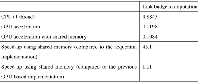
Testing the effect of the use of shared memory is done with same parameters as in Section 4.3, i.e. the simulation is run for 60 steps with 150,000 UTs. Then, the average time link budget computation takes in the simulation’s main loop is computed. Results are shown in Table 4.

Table 4.Time elapsed in seconds on average on link budget computations and speed-up achieved (ratio) using shared memory.

Link budget computation

CPU (1 thread) 4.8843

GPU acceleration 0.1198

GPU acceleration with shared memory 0.1084

Speed-up using shared memory (compared to the sequential implementation)

45.1

Speed-up using shared memory (compared to the previous GPU-based implementation)

1.11

When using shared memory the average time, with the parameters provided above, the link budget computation takes is 0.1084s. A speed-up of 1.11x compared to the previous GPU-based implementation was achieved. Compared to the sequential implementation the speed-up is 45.1x.

With the optimized version of the program, the simulations are run again with the same parameters as in Section 4.1, i.e. varying amounts of UTs in the system (10k, 50k, 100k, 150k, 200k, 500k and 1M) for 720 simulations steps, while the step size is ten seconds, so the total simulated time is two hours. Comparison of the results with the previous GPU-based implementation can be found in Table 5. The highest speed-up, compared to the sequential implementation, is still the one with 500k UTs. The speed-up is 16.0x.

Table 5.Total performance time in seconds and speed-up achieved (ratio) using shared memory.

10k 50k 100k 150k 200k 500k 1M

CPU (1 thread) 280 1248 2449 3658 4875 12187 24410

GPU acceleration 63 118 189 261 326 780 1594

GPU acceleration with shared memory

63 117 187 255 317 762 1562

Speed-up using shared memory (compared to the sequential implemen-tation)

4.4 10.7 13.1 14.3 15.4 16.0 15.6

Speed-up using shared memory (compared to the previous GPU-based implementation)

26

5

DISCUSSION

The results suggest that there is a great potential in using GPGPU in system simulations. The significance of this fact is due to that system simulations can be time consuming but with the aid of GPGPU one can accelerate simulations and increase performance of the development of the final product and thus save time and money.

As seen from Table 1, the greatest performance boost from the GPU accelerated imple-mentation compared to the sequential impleimple-mentation was achieved when 500k UTs in the system was used. Originally, the speed-up achieved was 15.6x and with the use of shared memory the speed-up increased to 16.0x (see Table 5). From Table 3 it can be seen that initially in the link budget computations with the baseline of 150k UTs a speed-up of 40.8x was achieved. After optimizing the program using shared memory, a speed-up of 45.1x in the link budget computations compared to the sequential implementation was achieved as well as a speed-up of 1.11x compared to the previous GPU-based implementation, as seen from Table 4. As it is suggested in [5], the shared memory should be made of good use and is a simple way to optimize a program that uses GPGPU.

In the implementation an assumption was made that the interference between the satellites is insignificant. Implementation taking into account the interference between the satellites is beyond the scope of this thesis and is part of the research in the future. In their hybrid network traffic model Liu et al. [26] studied ways to reduce transferring data between the host and the device. Future research could also include researching if there are ways to reduce transferring the data in the case of this simulator too.

6

CONCLUSION

The objective of this thesis was in the literature review to achieve general knowledge of GPGPU and apply that knowledge by implementing usage of GPGPU into a satellite network simulator. In the literature review, general knowledge of GPGPU was provided as well as a number of use cases for GPGPU in different applications and in system simulations were introduced. Usage of GPGPU was implemented to a satellite network simulator. A maximum total speed-up of 16.0x was achieved compared to a sequential implementation, as well as a speed-up of 45.1x in the link budget computations.

REFERENCES

[1] K. P. White and R. G. Ingalls. “THE BASICS OF SIMULATION”.2018 Winter Sim-ulation Conference (WSC). 2018, pp. 147–161.

[2] M. Singh. “Wireless networks: An overview”.SpringerBriefs in Applied Sciences and Technology. 2019, pp. 1–10.

[3] L. Djinevski, S. Filiposka, and D. Trajanov. “Network simulator tools and GPU par-allel systems”.Electronics. Vol. 16. 1. 2012, pp. 81–84.

[4] J. D. Owens, M. Houston, D. Luebke, S. Green, J. E. Stone, and J. C. Phillips. “GPU Computing”.Proceedings of the IEEE. Vol. 96. 5. 2008, pp. 879–899.

[5] C. A. Navarro, N. Hitschfeld-Kahler, and L. Mateu. “A survey on parallel computing and its applications in data-parallel problems using GPU architectures”. Communica-tions in Computational Physics. Vol. 15. 2. 2014, pp. 285–329.

[6] J. D. Owens, D. Luebke, N. Govindaraju, M. Harris, J. Kr¨uger, A. E. Lefohn, and T. J. Purcell. “A survey of general-purpose computation on graphics hardware”.Computer Graphics Forum. Vol. 26. 1. 2007, pp. 80–113.

[7] NVIDIA CUDA C Programming Guide Version 3.1.1. Accessed on: April 17, 2020. [Online]. Available: http://developer.download.nvidia.com/compute/ cuda/3 1/toolkit/docs/NVIDIA CUDA C ProgrammingGuide 3.1.pdf.

[8] Shane Cook.CUDA Programming: A Developer’s Guide to Parallel Computing with GPUs. 1st. San Francisco, CA, USA: Morgan Kaufmann Publishers Inc., 2012. [9] “CUDA Toolkit Documentation v10.2.89”. Accessed on: May 2, 2020. [Online].

Available: https://docs.nvidia.com/cuda/.

[10] “Khronos OpenCL Registry”. Accessed on: May 2, 2020. [Online]. Available: https://www.khronos.org/registry/OpenCL/.

[11] “High Performance Supercomputing — NVIDIA Tesla”. Accessed on: May 2, 2020. [Online]. Available: https://www.nvidia.com/en-us/data-center/tesla/.

[12] Raymond Tay. OpenCL Parallel Programming Development Cookbook. Packt Pub-lishing, 2013.

https://www.khronos.org/.

[14] “Compute Shader Overview”. Accessed on: May 2, 2020. [Online]. Available: https://docs.microsoft.com/fi-fi/windows/win32/direct3d11/direct3d-11-advanced-stages-compute-shader?redirectedfrom=MSDN.

[15] “Specification — OpenACC”. Accessed on: May 2, 2020. [Online]. Available: https://www.openacc.org/specification.

[16] X. Li, G. Zhang, H. H. Huang, Z. Wang, and W. Zheng. “Performance Analysis of GPU-Based Convolutional Neural Networks”. 2016 45th International Conference on Parallel Processing (ICPP). 2016, pp. 67–76.

[17] “Convolutional Neural Nets - Facebook Research”. Accessed on: May 2, 2020. [On-line]. Available: https://research.fb.com/videos/convolutional-neural-nets/.

[18] “ML Practicum: Image Classification — Machine Learning Practica”. Accessed on: May 2, 2020. [Online]. Available: https://developers.google.com/machine-learning/practica/image-classification.

[19] Alex Krizhevsky, Ilya Sutskever, and Geoffrey E. Hinton. “ImageNet Classifica-tion with Deep ConvoluClassifica-tional Neural Networks”. Commun. ACM 60.6 (May 2017), pp. 84–90.

[20] Ronan Collobert, Koray Kavukcuoglu, and Cl´ement Farabet. “Torch7: A Matlab-like Environment for Machine Learning”.NIPS 2011. 2011.

[21] T. M. Fern´andez-Caram´es and P. Fraga-Lamas. “A Review on the Use of Blockchain for the Internet of Things”.IEEE Access. Vol. 6. 2018, pp. 32979–33001.

[22] M. Bedford Taylor. “The Evolution of Bitcoin Hardware”.Computer. Vol. 50. 9. 2017, pp. 58–66.

[23] Joe Liebkind. “The GPU Industry is Booming Thanks to Blockchain”. Investopedia, 2018. Accessed on: Jan. 26, 2020. [Online]. Available: https://www.investopedia.com/ tech/gpu-industry-booming-thanks-blockchain/.

[24] Tim Kaldewey and Andrea Di Blas. “Chapter 1 - Large-Scale GPU Search”. GPU Computing Gems Jade Edition. Ed. by Wen-mei W. Hwu. Applications of GPU Com-puting Series. Boston: Morgan Kaufmann, 2012, pp. 3–14.

[25] Pawan Harish, P.J. Narayanan, Vibhav Vineet, and Suryakant Patidar. “Chapter 7 -Fast Minimum Spanning Tree Computation”. GPU Computing Gems Jade Edition. Ed. by Wen-mei W. Hwu. Applications of GPU Computing Series. Boston: Morgan Kaufmann, 2012, pp. 77–88.

[26] J. Liu, Y. Liu, Z. Du, and T. Li. “GPU-assisted hybrid network traffic model”. SIGSIM-PADS 2014 - Proceedings of the 2014 ACM Conference on SIGSIM Principles of Advanced Discrete Simulation. 2014, pp. 63–74.

[27] P. -Y Lucas, N. H. Van Long, T. P. Truong, and B. Pottier. “Wireless sensor networks and satellite simulation”.Lecture Notes of the Institute for Computer Sciences, Social-Informatics and Telecommunications Engineering, LNICST. Vol. 154. 2015, pp. 185– 198.

[28] B. R. Bilel and N. Navid. “Cunetsim: A GPU based simulation testbed for large scale mobile networks”.2012 International Conference on Communications and Informa-tion Technology (ICCIT). June 2012, pp. 374–378.

[29] J. Ivey, G. Riley, B. Swenson, and M. Loper. “Designing and enabling simulation of real-world GPU network applications with ns-3 and DCE”. Institute of Electrical and Electronics Engineers Inc., 2016, pp. 445–450.

[30] “The gVirtuS Open Source Project on Open Hub”. Accessed on: May 7, 2020. [On-line]. Available: https://www.openhub.net/p/gvirtus.

[31] Sassan Ahmadi. “Chapter 11 - Link-Level and System-Level Performance of LTE-Advanced”.LTE-Advanced. Academic Press, 2014, pp. 875–949.

[32] “Numba documentation”. Accessed on: April 1, 2020. [Online]. Available: http://numba. pydata.org/numba-doc/latest/index.html.

[33] “TESLA K80 GPU ACCELERATOR”. Accessed on: April 3, 2020. [Online]. Available: https://www.nvidia.com/content/dam/en-zz/Solutions/Data-Center/tesla-product-literature/Tesla-K80-BoardSpec-07317-001-v05.pdf.

[34] F. D´evai. “The Refutation of Amdahl’s Law and Its Variants”.Transactions on Com-putational Science XXXIII. Berlin, Heidelberg: Springer Berlin Heidelberg, 2018, pp. 79–96.

1 @cuda.jit

2 def link_budget_cuda(result, uts, sats):

3 """

4 Compute link budget using GPU. Each thread on the device

computes a UT's link budget to a satellite.

,→

5

6 @param result:

(numba.cuda.cudadrv.devicearray.DeviceNDArray) Device array into which the link budgets will be stored.

,→

,→

7 @param uts: (numba.cuda.cudadrv.devicearray.DeviceNDArray)

Device array of UTs.

,→

8 @param sats: (numba.cuda.cudadrv.devicearray.DeviceNDArray)

Device array of satellites.

,→

9 """ 10

11 j, k = cuda.grid(2) # global indices of the thread 12 n_uts = uts.shape[0]

13 n_sats = sats.shape[0] 14

15 if (j >= n_uts) | (k >= n_sats):

16 return

17

18 earth_radius = 6371 * 1000 # m

19 freq = 29.75*10**9 # center frequency (Hz) 20 alt = sats[k][2] _{* 1000} # m

21

22 # get needed angles

23 bearing_angle = compute_bearing_angle(uts[j][1], uts[j][0],

sats[k][0], sats[k][1], alt) ,→

24 max_earth_angle_seen_by_satellite = compute_max_earth_angle_seen_by_satellite(earth_radius, alt) ,→ ,→ 25 angular_earth_radius = compute_angular_earth_radius(earth_radius, alt) ,→ 26 nadir_angle = compute_nadir_angle(angular_earth_radius, bearing_angle) ,→ 27 elevation_angle = compute_elevation_angle(bearing_angle, nadir_angle) ,→ 28

29 C = compute_link_budget(bearing_angle, alt, freq)

30 if (elevation_angle/2/math.pi_{*360 > 20}) | (bearing_angle >

max_earth_angle_seen_by_satellite): ,→

31 C = -math.inf # elevation angles greater than 20 is not

permitted, thus link budget is -inf dBm

,→

32 result[j][k] = C # dBm

Calling the link budget computation from the host happens as follows.

1 simulate_gpu.link_budget_cuda[(N_UTS//8+1, len(sats)//8+1), (8,

8)](link_budgets_gpu, uts_gpu, sats_gpu) ,→

shared memory

1 @cuda.jit

2 def link_budget_cuda(result, uts, sats):

3 ...

4 x = cuda.grid(1) # global indices of the thread 5

6 if x >= n_uts:

7 return

8

9 tx = cuda.threadIdx.x # index inside the block 10 n_uts = uts.shape[0]

11 n_sats = sats.shape[0]

12 # define shared array that will contain data of the

satellites

,→

13 sA = cuda.shared.array(shape=(198, 3), dtype=float32) 14

15 if (tx < sats.shape[0]):

16 for i in range(0, sats.shape[1]): 17 sA[tx][i] = sats[tx][i]

18

19 cuda.syncthreads() 20

21 earth_radius = 6371 * 1000 # km

22 freq = 29.75*10**9 # center frequency (Hz) 23

24 for i in range(0, n_sats): 25 alt = sA[i][2] _{* 1000} # km 26

27 # get needed angles

28 bearing_angle = compute_bearing_angle(uts[x][1],

uts[x][0], sA[i][0], sA[i][1], alt) ,→

29 max_earth_angle_seen_by_satellite = compute_max_earth_angle_seen_by_satellite( earth_radius, alt) ,→ ,→ 30 angular_earth_radius = compute_angular_earth_radius(earth_radius, alt) ,→ 31 nadir_angle = compute_nadir_angle(angular_earth_radius, bearing_angle) ,→ 32 elevation_angle = compute_elevation_angle(bearing_angle, nadir_angle) ,→ 33

34 C = compute_link_budget(bearing_angle, alt, freq) 35 if (elevation_angle/2/math.pi_{*360 > 20}) |

(bearing_angle >

max_earth_angle_seen_by_satellite): ,→

,→

36 C = -math.inf # elevation angles greater than 20 is

not permitted, thus link budget is -inf dB

,→

37 result[x][i] = C # dB

Calling the link budget computation from the host happens as follows.

1 block_size = (sats.shape[0]//32+1)_*32

2 simulate_gpu.link_budget_cuda[N_UTS//block_size+1,

block_size](link_budgets_gpu, uts_gpu, sats_gpu) ,→