Documentation
January 21, 2016
Apache, Apache Cassandra, Apache Hadoop, Hadoop and the
eye logo are trademarks of the Apache Software Foundation
Contents
Introduction to Cassandra Query Language... 6
CQL data modeling...6
Data modeling concepts...7
Data modeling analysis... 9
Using CQL... 9
Starting cqlsh...10
Starting cqlsh on Linux and Mac OS X... 10
Starting cqlsh on Windows...10
Creating and updating a keyspace... 11
Example of creating a keyspace... 11
Updating the replication factor... 12
Creating a table...12
Creating a table... 12
Using the keyspace qualifier... 14
Simple Primary Key... 15
Composite Partition Key... 16
Compound Primary Key... 17
Creating a counter table...18
Create table with COMPACT STORAGE...20
Table schema collision fix... 20
Creating a materialized view...20
Creating advanced data types in tables... 22
Creating collections... 23
Creating a table with a tuple... 25
Creating a user-defined type (UDT)... 25
Creating functions...26
Create user-defined function (UDF)... 26
Create User-Defined Aggregate Function (UDA)... 27
Inserting and updating data... 27
Inserting simple data into a table... 27
Inserting and updating data into a set... 28
Inserting and updating data into a list...29
Inserting and updating data into a map... 30
Inserting tuple data into a table... 31
Inserting data into a user-defined type (UDT)...31
Inserting JSON data into a table...32
Using lightweight transactions... 32
Expiring data with Time-To-Live...33
Expiring data with TTL example...33
Inserting data using COPY and a CSV file...34
Retrieval and sorting results...38
Retrieval using collections... 40
Retrieval using JSON... 41
Retrieval using the IN keyword... 41
Retrieval by scanning a partition...42
Retrieval using standard aggregate functions... 43
Retrieval using a user-defined function (UDF)... 44
Retrieval using user-defined aggregate (UDA) functions... 44
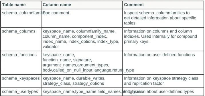
Querying a system table... 45
Indexing tables... 49
Indexing...49
Building and maintaining indexes...53
Altering a table... 54
Altering columns in a table...54
Altering a table to add a collection... 54
Altering the data type of a column...55
Altering a materialized view... 55
Altering a user-defined type... 55
Removing a keyspace, schema, or data... 56
Dropping a keyspace, table or materialized view... 56
Deleting columns and rows... 56
Dropping a user-defined function (UDF)... 57
Securing a table... 57
Database users...57
Database roles...58
Database Permissions... 59
Tracing consistency changes... 60
Setup to trace consistency changes... 61
Trace reads at different consistency levels...62
How consistency affects performance...67
Paging through an unordered partitioner... 67
Determining time-to-live for a column... 69
Determining the date/time of a write...70
Legacy tables... 71
Working with legacy applications... 71
Querying a legacy table... 71
Using a CQL legacy table query...71
CQL reference... 72
Introduction... 72
CQL lexical structure... 72
Uppercase and lowercase... 73
Escaping characters... 74 Valid literals... 74 Exponential notation... 75 CQL code comments...75 CQL Keywords...75 CQL data types... 79 Blob type...80 Collection type... 81 Counter type... 82
UUID and timeuuid types... 82
User-defined type... 85
CQL keyspace and table properties... 86
Table properties... 86 Compaction subproperties... 89 Compression subproperties... 92 Functions... 93 CQL limits... 94 cqlsh commands...94 cqlsh... 94 CAPTURE... 97 CLEAR... 98 CONSISTENCY... 98 COPY... 99 DESCRIBE... 105 EXPAND... 107 EXIT... 107 PAGING... 108 SERIAL CONSISTENCY... 108 SHOW... 109 SOURCE... 110 TRACING... 111 CQL commands...115 ALTER KEYSPACE... 115
ALTER MATERIALIZED VIEW...116
ALTER ROLE... 117 ALTER TABLE... 118 ALTER TYPE... 121 ALTER USER... 123 BATCH... 123 CREATE AGGREGATE...126 CREATE INDEX... 126 CREATE FUNCTION...129 CREATE KEYSPACE... 130
CREATE MATERIALIZED VIEW...133
CREATE TABLE... 134 CREATE TRIGGER... 139 CREATE ROLE... 140 CREATE USER... 141 DELETE... 142 DESCRIBE... 144 DROP AGGREGATE...146 DROP FUNCTION... 146 DROP INDEX... 147 DROP KEYSPACE... 147
DROP MATERIALIZED VIEW...148
DROP ROLE...149 DROP TABLE... 149 DROP TRIGGER... 150 DROP TYPE... 150 DROP USER... 151 GRANT...151
SELECT... 160
TRUNCATE...168
UPDATE...168
USE... 172
Introduction to Cassandra Query Language
Cassandra Query Language (CQL) is a query language for the Cassandra database.Cassandra Query Language (CQL) is a query language for the Cassandra database.
The Cassandra Query Language (CQL) is the primary language for communicating with the Cassandra database. The most basic way to interact with Cassandra is using the CQL shell, cqlsh. Using cqlsh, you can create keyspaces and tables, insert and query tables, plus much more. If you prefer a graphical tool, you can use DataStax DevCenter. For production, DataStax supplies a number of drivers so that CQL statements can be passed from client to cluster and back. Other administrative tasks can be accomplished using OpsCenter.
Important: This document assumes you are familiar with the Cassandra 2.2 documentation, Cassandra 3.0 documentation or Cassandra 3.x documentation.
Table: CQL for Cassandra 2.2 and later features New CQL features
include:
• JSON support for CQL3 • User Defined Functions (UDFs) • User Defined Aggregates (UDAs) • Role Based Access Control (RBAC) • Native Protocol v.4
• In Cassandra 3.0 and later, Materialized Views • Addition of CLEAR command for cqlsh
Improved CQL features include:
• Additional COPY command options • New CREATE TABLE WITH ID command
• Support IN clause on any partition key column or clustering column • Accept Dollar Quoted Strings
• Allow Mixing Token and Partition Key Restrictions • Support Indexing Key/Value Entries on Map Collections
• Date data type added and improved time/date conversion functions • Change to CREATE TABLE syntax for compression options Removed CQL features
include:
• Removal of CQL2 • Removal of cassandra-cli
Native protocol The Native Protocol has been updated to version 4, with implications for CQL use in the DataStax drivers.
CQL data modeling
Data modeling topics.Note: DataStax Academy provides a course in Cassandra data modeling. This course presents
Data modeling concepts
How data modeling should be approached for Cassandra. A Pro Cycling statistics example is used throughout the CQL document.Data modeling is a process that involves identifying the entities (items to be stored) and the relationships between entities. To create your data model, identify the patterns used to access data and the types of queries to be performed. These two ideas inform the organization and structure of the data, and the design and creation of the database's tables. Indexing the data can improve performance in some cases, so decide which columns will have secondary indexes.
Data modeling in Cassandra uses a query-driven approach, in which specific queries are the key to organizing the data. Queries are the result of selecting data from a table; schema is the definition of how data in the table is arranged. Cassandra's database design is based on the requirement for fast reads and writes, so the better the schema design, the faster data is written and retrieved.
In contrast, relational databases normalize data based on the tables and relationships designed, and then writes the queries that will be made. Data modeling in relational databases is table-driven, and any relationships between tables are expressed as table joins in queries.
Cassandra's data model is a partitioned row store with tunable consistency. Tunable consistency means for any given read or write operation, the client application decides how consistent the requested data must be. Rows are organized into tables; the first component of a table's primary key is the partition key; within a partition, rows are clustered by the remaining columns of the key. Other columns can be indexed separately from the primary key. Because Cassandra is a distributed database, efficiency is gained for reads and writes when data is grouped together on nodes by partition. The fewer partitions that must be queried to get an answer to a question, the faster the response. Tuning the consistency level is another factor in latency, but is not part of the data modeling process.
Cassandra data modeling focuses on the queries. Throughout this topic, the example of Pro Cycling statistics demonstrates how to model the Cassandra table schema for specific queries. The conceptual model for this data model shows the entities and relationships.
The entities and their relationships are considered during table design. Queries are best designed to access a single table, so all entities involved in a relationship that a query encompasses must be in the table. Some tables will involve a single entity and its attributes, like the first example shown below. Others
in two or more tables and foreign keys would be used to relate the data between the tables. Because Cassandra uses this single table-single query approach, queries can perform faster.
One basic query (Q1) for Pro Cycling statistics is a list of cyclists, including each cyclist's id, firstname, and lastname. To uniquely identify a cyclist in the table, an id using UUID is used. For a simple query to list all cyclists a table that includes all the columns identified and a partition key (K) of id is created. The diagram below shows a portion of the logical model for the Pro Cycling data model.
Figure: Query 1: Find a cyclist's name with a specified id
A related query (Q2) searches for all cyclists by a particular race category. For Cassandra, this query is more efficient if a table is created that groups all cyclists by category. Some of the same columns are required (id, lastname), but now the primary key of the table includes category as the partition key (K), and groups within the partition by the id (C). This choice ensures that unique records for each cyclist are created.
Figure: Query 2: Find cyclists given a specified category
These are two simple queries; more examples will be shown to illustrate data modeling using CQL. Notice that the main principle in designing the table is not the relationship of the table to other tables, as it is in relational database modeling. Data in Cassandra is often arranged as one query per table, and data is repeated amongst many tables, a process known as denormalization. Relational databases instead normalize data, removing as much duplication as possible. The relationship of the entities is important, because the order in which data is stored in Cassandra can greatly affect the ease and speed of data retrieval. The schema design captures much of the relationship between entities by including related attributes in the same table. Client-side joins in application code is used only when table schema cannot
Data modeling analysis
How to analyze a logical data model.You've created a conceptual model of the entities and their relationships. From the conceptual model, you've used the expected queries to create table schema. The last step in data model involves completing an analysis of the logical design to discover modifications that might be needed. These modifications can arise from understanding partition size limitations, cost of data consistency, and performance costs due to a number of design choices still to be made.
For efficient operation, partitions must be sized within certain limits. Two measures of partition size are the number of values in a partition and the partition size on disk. The maximum number of columns per row is two billion. Sizing the disk space is more complex, and involves the number of rows and the number of columns, primary key columns and static columns in each table. Each application will have different efficiency parameters, but a good rule of thumb is to keep the maximum number of values below 100,000 items and the disk size under 100MB.
Data redundancy must be considered as well. Two redundancies that are a consequence of Cassandra's distributed design are duplicate data in tables and multiple partition replicates.
Data is generally duplicated in multiple tables, resulting in performance latency during writes and requires more disk space. Consider storing a cyclist's name and id in more than one data, along with other items like race categories, finished races, and cyclist statistics. Storing the name and id in multiple tables results in linear duplication, with two values stored in each table. Table design must take into account the possibility of higher order duplication, such as unlimited keywords stored in a large number of rows. A case of n keywords stored in m rows is not a good table design. You should rethink the table schema for better design, still keeping the query foremost.
Cassandra replicates partition data based on the replication factor, using more disk space. Replication is a necessary aspect of distributed databases and sizing disk storage correctly is important.
Application-side joins can be a performance killer. In general, you should analyze your queries that require joins and consider pre-computing and storing the join results in an additional table. In Cassandra, the goal is to use one table per query for performant behavior. Lightweight transactions (LWT) can also affect performance. Consider whether or not the queries using LWT are necessary and remove the requirement if it is not strictly needed.
Using CQL
CQL provides an API to Cassandra that is simpler than the Thrift API.CQL provides an API to Cassandra that is simpler than the Thrift API. The Thrift API and legacy versions of CQL expose the internal storage structure of Cassandra. CQL adds an abstraction layer that hides implementation details of this structure and provides native syntaxes for collections and other common encodings.
Accessing CQL
Common ways to access CQL are:
• Start cqlsh, the Python-based command-line client, on the command line of a Cassandra node. • Use DataStax DevCenter, a graphical user interface.
• For developing applications, you can use one of the official DataStax C#, Java, or Python open-source drivers.
• Use the set_cql_version Thrift method for programmatic access. This document presents examples using cqlsh.
Starting cqlsh
How to start cqlsh.Starting cqlsh on Linux and Mac OS X
A brief description on starting cqlsh on Linux and Mac OS X.This procedure briefly describes how to start cqlsh on Linux and Mac OS X. The cqlsh command is covered in detail later.
Procedure
1. Navigate to the Cassandra installation directory. 2. Start cqlsh on the Mac OSX, for example.
$ bin/cqlsh
If you use security features, provide a user name and password.
3. Optionally, specify the IP address and port to start cqlsh on a different node. $ bin/cqlsh 1.2.3.4 9042
Note: You can use tab completion to see hints about how to complete a cqlsh command. Some platforms, such as Mac OSX, do not ship with tab completion installed. You can use easy_install to install tab completion capabilities on Mac OSX:
$ easy_install readline
Starting cqlsh on Windows
A brief description on starting cqlsh on Windows.This procedure describes how to start cqlsh on Windows. The P command is covered in detail later.
Procedure
You can start cqlsh in two ways: • From the Start menu:
a) Navigate to Start > Programs > DataStax Distribution of Apache Cassandra.
b) If using Cassandra 3.0+, click DataStax Distribution of Apache Cassandra > Cassandra CQL Shell
c) If using Cassandra 2.2, click DataStax Community Edition > Cassandra CQL Shell. The cqlsh prompt appears: cqlsh>
• From the Command Prompt: a) Open the Command Prompt.
b) Navigate to Cassandra bin directory: Cassandra 3.0+:
To start cqlsh on a different node, add the IP address and port: C:\> cqlsh 1.2.3.4 9042
Note: You can use tab completion to see hints about how to complete a cqlsh command. To install tab completion capabilities on Windows, you can use pip install pyreadline.
Creating and updating a keyspace
Creating a keyspace is the CQL counterpart to creating an SQL database.Creating a keyspace is the CQL counterpart to creating an SQL database, but a little different. The
Cassandra keyspace is a namespace that defines how data is replicated on nodes. Typically, a cluster has one keyspace per application. Replication is controlled on a per-keyspace basis, so data that has different replication requirements typically resides in different keyspaces. Keyspaces are not designed to be used as a significant map layer within the data model. Keyspaces are designed to control data replication for a set of tables.
When you create a keyspace, specify a strategy class for replicating keyspaces. Using the
SimpleStrategy class is fine for evaluating Cassandra. For production use or for use with mixed workloads, use the NetworkTopologyStrategy class.
To use NetworkTopologyStrategy for evaluation purposes using, for example, a single node cluster, the default data center name is used. To use NetworkTopologyStrategy for production use, you need to change the default snitch, SimpleSnitch, to a network-aware snitch, define one or more data center names in the snitch properties file, and use the data center name(s) to define the keyspace; see Snitch. For example, if the cluster uses the PropertyFileSnitch, create the keyspace using the user-defined data center and rack names in the cassandra-topologies.properties file. If the cluster uses the Ec2Snitch, create the keyspace using EC2 data center and rack names. If the cluster uses the GoogleCloudSnitch, create the keyspace using GoogleCloud data center and rack names.
If you fail to change the default snitch and use NetworkTopologyStrategy, Cassandra will fail to complete any write request, such as inserting data into a table, and log this error message:
Unable to complete request: one or more nodes were unavailable.
Note: You cannot insert data into a table in keyspace that uses NetworkTopologyStrategy unless you define the data center names in the snitch properties file or you use a single data center named datacenter1.
Example of creating a keyspace
A simple example of querying Cassandra by creating a keyspace and then using it.To query Cassandra, create and use a keyspace. Choose an arbitrary data center name and register the name in the properties file of the snitch. Alternatively, in a cluster in a single data center, use the default data center name, for example, datacenter1, and skip registering the name in the properties file.
Procedure
1. Determine the default data center name, if using NetworkTopologyStrategy, using nodetool status. $ bin/nodetool status
The output is:
|/ State=Normal/Leaving/Joining/Moving
-- Address Load Tokens Owns (effective) Host ID Rack UN 127.0.0.1 41.62 KB 256 100.0% 75dcca8f... rack1 2. Create a keyspace.
cqlsh> CREATE KEYSPACE IF NOT EXISTS cycling WITH REPLICATION = { 'class' : 'NetworkTopologyStrategy', 'datacenter1' : 3 }; 3. Use the keyspace.
cqlsh> USE cycling;
Updating the replication factor
Increasing the replication factor increases the total number of copies of keyspace data stored in a Cassandra cluster.Increasing the replication factor increases the total number of copies of keyspace data stored in a Cassandra cluster. If you are using security features, it is particularly important to increase the replication factor of the system_auth keyspace from the default (1) because you will not be able to log into the cluster if the node with the lone replica goes down. It is recommended to set the replication factor for the system_auth keyspace equal to the number of nodes in each data center.
Procedure
1. Update a keyspace in the cluster and change its replication strategy options. cqlsh> ALTER KEYSPACE system_auth WITH REPLICATION =
{'class' : 'NetworkTopologyStrategy', 'dc1' : 3, 'dc2' : 2}; Or if using SimpleStrategy:
cqlsh> ALTER KEYSPACE "Excalibur" WITH REPLICATION =
{ 'class' : 'SimpleStrategy', 'replication_factor' : 3 }; 2. On each affected node, run the nodetool repair command.
3. Wait until repair completes on a node, then move to the next node.
Creating a table
How to create tables to store data.In CQL, data is stored in tables containing rows of columns.
Creating a table
How to create CQL tables.In CQL, data is stored in tables containing rows of columns, similar to SQL definitions.
Note: The concept of rows and columns in the internal implementation of Cassandra are not the same. For more information, see A thrift to CQL3 upgrade guide or CQL3 for Cassandra experts.
Tables can be created, dropped, and altered at runtime without blocking updates and queries. When you create a table, define a primary key and columns along with table properties. Use the optional WITH clause and keyword arguments to configure table properties: caching, compaction, and other operations. Table
Create schema using cqlsh
Create table schema using cqlsh. Dynamic schema generation is not supported; collision can occur if multiple clients attempt to generate tables simultaneously. To fix problems if you do accidentally have collision occur, see the schema collision fix instructions.
Primary Key
A primary key identifies the location and order of data storage. The primary key is defined at table creation time and cannot be altered. If the primary key must be changed, a new table schema is created and the data is written to the new table. Cassandra is a partition row store, and a component of the primary key, the partition key, identifies which node will hold a particular table row. See ALTER TABLE for details on altering a table after creation.
At the minimum, the primary key must consist of a partition key. Composite partition keys can split a data set so that related data is stored on separate partitions. Compound primary keys include clustering columns which order the data on a partition.
The definition of a table's primary key is critical in Cassandra. Carefully model how data in a table will be inserted and retrieved before choosing which columns will define the primary key. The size of the partitions, the order of the data within partitions, the distribution of the partitions amongst the nodes of the cluster - all of these considerations determine selection of the best primary key for a table.
Table characteristics
Valid table names are strings of alphanumeric characters and underscores that begin with a letter. To specify a table name:
• Use dot notation to specify the table name. Create a table using the keyspace name separated from the table name with a period. The keyspace remains in the current keyspace, but creates the table in the specified keyspace.
• Use the current keyspace. Create a table using only the table name.
Column characteristics
Columns are an essential component of a CQL table. Several column types exist to afford flexibility to table schema design. Each column in a table is assigned a data type during table creation. Column types, other than collection-type columns, are specified as a parenthesized, comma-separated list of column name and type pairs. The following example illustrates three data types, UUID, text and timestamp:
CREATE TABLE cycling.cyclist_alt_stats ( id UUID PRIMARY KEY, lastname text, birthday timestamp, nationality text, weight text, height text );
Collection column types supported are map, set, and list. A collection column is declared using the collection type, followed by another type, such as int or text, in angle brackets. Like other columns, collection columns are specified as a parenthesized, comma-separated list of column name and type pair. The following example illustrates each collection type, but is not designed for an actual query:
CREATE TABLE cycling.whimsey ( id UUID PRIMARY KEY, lastname text, cyclist_teams set<text>, events list<text>, teams map<int,text> );
Collection types cannot currently be nested. Collections can include a frozen data type. For examples and usage, see Collection type on page 81
The column type tuple data type holds fixed-length sets of typed positional fields. Use a tuple as an alternative to a user-defined type. A tuple can accommodate many fields (32768), more than can be prudently used. Typically, create a tuple with a small number of fields. A tuple is typically used for 2 to 5 fields. To create a tuple in a table, use angle brackets and a comma delimiter to declare the tuple
component types. Tuples can be nested. The following example illustrates a tuple type composed of a text field and a nested tuple of two float fields:
CREATE TABLE cycling.route (race_id int, race_name text, point_id int,
lat_long tuple<text, tuple<float,float>>, PRIMARY KEY (race_id, point_id)); Note: Cassandra 2.1.0 to 2.1.2 requires using frozen for tuples, while Cassandra 2.1.3 and later does not require this keyword:
frozen <tuple <int, tuple<text, double>>> For more information, see "Tuple type".
User-defined types (UDTs) can be used for a column type when a data type of several fields was created using CREATE TYPE. A UDT is created when it will be used for multiple table definitions. The column type user-defined type (UDT) requires the frozen keyword. A frozen value serializes multiple components into a single value. Non-frozen types allow updates to individual fields. Cassandra treats the value of a frozen type as a blob. The entire value must be overwritten. The scope of a user-defined type is the keyspace in which you define it. Use dot notation to access a type from a keyspace outside its scope: keyspace name followed by a period followed the name of the type. Cassandra accesses the type in the specified keyspace, but does not change the current keyspace; otherwise, if you do not specify a keyspace, Cassandra accesses the type within the current keyspace. For examples and usage information, see "Using a user-defined type".
A counter is a special column used to store a number that is changed in increments. A counter can only be used in a dedicated table that includes a column of counter data type. For more examples and usage information, see "Using a counter".
Using the keyspace qualifier
To simplify tracking multiple keyspaces, use the keyspace qualifier instead of the USE statement.Sometimes issuing a USE statement to select a keyspace is inconvenient. Connection pooling requires managing multiple keyspaces. To simplify tracking multiple keyspaces, use the keyspace qualifier instead of the USE statement. You can specify the keyspace using the keyspace qualifier in these statements: • ALTER TABLE • CREATE TABLE • DELETE • INSERT • SELECT • TRUNCATE • UPDATE
Procedure
To specify a table when you are not in the keyspace that contains the table, use the name of the keyspace followed by a period, then the table name. For example, cycling.race_winners.
cqlsh> INSERT INTO cycling.race_winners ( race_name, race_position, cyclist_name ) VALUES (
'National Championships South Africa WJ-ITT (CN)', 1,
Simple Primary Key
A simple primary key consists of only the partition key which determines which node stores the data.For a table with a simple primary key, Cassandra uses one column name as the partition key. The primary key consists of only the partition key in this case. If a large amount of data will be ingested, but few values will be inserted for the column that defines the primary key, the partitions can grow large. Large partitions might be slow to respond to read requests, or grow too large for a node's assigned disk space. On the other hand, data stored with a simple primary key will be fast to insert and retrieve if many values for the column can distribute the partitions across many nodes.
Often, your first venture into using Cassandra involves tables with simple primary keys. Keep in mind that only the primary key can be specified when retrieving data from the table, if secondary indexes are not used. Many production tables will use as some unique identifier as a simple primary key. Look up the identifier and the rest of the data in the table is retrieved. If an application needs a simple lookup table, use a simple primary key. The table shown uses id as the primary key.
To create a table having a single primary key, two methods can be used:
• Insert the PRIMARY KEY keywords after the column name in the CREATE TABLE definition. • Insert the PRIMARY KEY keywords after the last column definition in the CREATE TABLE definition,
followed by the column name of the key. The column name is enclosed in parentheses.
Using a simple primary key
Use a simple primary key to create columns that you can query to return sorted results.Use a simple primary key to create columns that you can query to return sorted results. This example creates a cyclist_name table storing an ID number and a cyclist's first and last names in columns. The table uses a UUID as a primary key. This table can be queried to discover the name of a cyclist given their ID number.
A simple primary key table can be created in three different ways, as shown.
Procedure
• Create the table cyclist_name in the cycling keyspace, making id the primary key. Before creating the table, set the keyspace with a USE statement.
cqlsh> USE cycling;
CREATE TABLE cyclist_name ( id UUID PRIMARY KEY, lastname text, firstname text );
• This same example can be written with the primary key identified at the end of the table definition. cqlsh> USE cycling;
CREATE TABLE cyclist_name ( id UUID, lastname text, firstname text, PRIMARY KEY (id) );
• The keyspace name can be used to identify the keyspace in the CREATE TABLE statement instead of the USE statement.
cqlsh> CREATE TABLE cycling.cyclist_name ( id UUID, lastname text, firstname text, PRIMARY KEY (id) );
• Cassandra 2.2 and later can use a date or time data type.
CREATE TABLE cycling.birthdays (id UUID PRIMARY KEY, bday date, btime time);
Composite Partition Key
A partition key can have a partition key defined with multiple table columns which determines which node stores the data.For a table with a composite partition key, Cassandra uses multiple columns as the partition key. These columns form logical sets inside a partition to facilitate retrieval. In contrast to a simple partition key, a composite partition key uses two or more columns to identify where data will reside. Composite partition keys are used when the data stored is too large to reside in a single partition. Using more than one column for the partition key breaks the data into chunks, or buckets. The data is still grouped, but in smaller chunks. This method can be effective if a Cassandra cluster experiences hotspotting, or
congestion in writing data to one node repeatedly, because a partition is heavily writing. Cassandra is often used for time series data, and hotspotting can be a real issue. Breaking incoming data into buckets by year:month:day:hour, using four columns to route to a partition can decrease hotspots.
Data is retrieved using the partition key. Keep in mind that to retrieve data from the table, values for all columns defined in the partition key have to be supplied, if secondary indexes are not used. The table shown uses race_year and race_name in the primary key, as a composition partition key. To retrieve data, both parameters must be identified.
To create a table having a composite partition key, use the following method:
• Insert the PRIMARY KEY keywords after the last column definition in the CREATE TABLE definition, followed by the column names of the partition key. The column names for the composite partition key are enclosed in double parentheses.
Cassandra stores an entire row of data on a node by partition key. If you have too much data in a partition and want to spread the data over multiple nodes, use a composite partition key.
Using a composite partition key
Use a composite partition key to identify where data will be stored.Use a composite partition key in your primary key to create columns that you can query to return sorted results. This example creates a rank_by_year_and_name table storing the ranking and name of
Procedure
• Create the table rank_by_year_and_name in the cycling keyspace. Use race_year and race_name for the composite partition key. The table definition shown has an additional column rank used in the primary key. Before creating the table, set the keyspace with a USE statement. This example identifies the primary key at the end of the table definition. Note the double parentheses around the first two columns defined in the PRIMARY KEY.
cqlsh> USE cycling;
CREATE TABLE rank_by_year_and_name ( race_year int,
race_name text, cyclist_name text, rank int,
PRIMARY KEY ((race_year, race_name), rank) );
• The keyspace name can be used to identify the keyspace in the CREATE TABLE statement instead of the USE statement.
cqlsh> CREATE TABLE cycling.rank_by_year_and_name ( race_year int,
race_name text, cyclist_name text, rank int,
PRIMARY KEY ((race_year, race_name), rank) );
Compound Primary Key
A compound primary key consists of a partition key that determines which node stores the data and of clustering column(s) which determine the order of the data on the partition.For a table with a compound primary key, Cassandra uses a partition key that is either simple or
composite. In addition, clustering column(s) are defined. Clustering is a storage engine process that sorts data within each partition based on the definition of the clustering columns. Normally, columns are sorted in ascending alphabetical order. Generally, a different grouping of data will benefit reads and writes better than this simplistic choice.
Remember that data is distributed throughout the Cassandra cluster. An application can experience high latency while retrieving data from a large partition if the entire partition must be read to gather a small amount of data. On a physical node, when rows for a partition key are stored in order based on the clustering columns, retrieval of rows is very efficient. Grouping data in tables using clustering columns is the equivalent of JOINs in a relational database, but are much more performant because only one table is accessed. This table uses category as the partition key and points as the clustering column. Notice that for each category, the points are ordered in descending order.
• Insert the PRIMARY KEY keywords after the last column definition in the CREATE TABLE definition, followed by the column name of the key. The column name is enclosed in parentheses.
Using a compound primary key
Use a compound primary key to create columns that you can query to return sorted results.Use a compound primary key to create columns that you can query to return sorted results. If our pro cycling example was designed in a relational database, you would create a cyclists table with a foreign key to the races. In Cassandra, you denormalize the data because joins are not performant in a distributed system. Later, other schema are shown that improve Cassandra performance. Collections and indexes are two data modeling methods. This example creates a cyclist_category table storing a cyclist's last name, ID, and points for each type of race category. The table uses category for the partition key and points for a single clustering column. This table can be queried to retrieve a list of cyclists and their points in a category, sorted by points.
A compound primary key table can be created in two different ways, as shown.
Procedure
• To create a table having a compound primary key, use two or more columns as the primary key. This example uses an additional clause WITH CLUSTERING ORDER BY to order the points in descending order. Ascending order is more efficient to store, but descending queries are faster due to the nature of the storage engine.
cqlsh> USE cycling;
CREATE TABLE cyclist_category ( category text,
points int, id UUID,
lastname text,
PRIMARY KEY (category, points)
) WITH CLUSTERING ORDER BY (points DESC);
• The keyspace name can be used to identify the keyspace in the CREATE TABLE statement instead of the USE statement.
cqlsh> CREATE TABLE cyclist_category ( category text,
points int, id UUID,
lastname text,
PRIMARY KEY (category, points)
) WITH CLUSTERING ORDER BY (points DESC);
Note: The combination of the category and points uniquely identifies a row in the cyclist_category table. More than one row with the same category can exist as long as the rows contain different pointsvalues. Consider the example again; is the data modeling for storing this data optimal? Under what conditions might errors occur?
Creating a counter table
A counter is a special column for storing a number that is changed in increments.Counters are useful for many data models. For example, a company may wish to keep track of the number of web page views received on a company website. Scorekeeping applications could use a counter to keep
Tracking count in a distributed database presents an interesting challenge. In Cassandra, the counter value will be located in the Memtable, commit log, and one or more SSTables at any given moment. Replication between nodes can cause consistency issues in certain edge cases. Cassandra counters were redesigned in Cassandra 2.1 to alleviate some of the difficulties. Read "What’s New in Cassandra 2.1: Better Implementation of Counters" to discover the improvements made in the counters.
A counter is a special column used to store a number that is changed in increments. A counter can be decremented or incremented in integer values. Because counters are implemented differently from other columns, counter columns can only be defined in dedicated tables. The counter data type is used to set the data type. Do not assign this type to a column that serves as the primary key or partition key. Also, do not use the counter type in a table that contains anything other than counter types and the primary key. Explicitly, the only non-counter columns in a counter table must be part of the primary key.
Many counter-related settings can be set in the cassandra.yaml file.
A counter column cannot be indexed or deleted.. To load data into a counter column, or to increase or decrease the value of the counter, use the UPDATE command. Cassandra rejects USING TIMESTAMP or USING TTL when updating a counter column.
To create a table having one or more counter columns, use this:
• Use CREATE TABLE to define the counter and non-counter columns. Use all non-counter columns as part of the PRIMARY KEY definition.
Using a counter
A counter is a special column for storing a number that is changed in increments.To load data into a counter column, or to increase or decrease the value of the counter, use the UPDATE command. Cassandra rejects USING TIMESTAMP or USING TTL in the command to update a counter column.
Procedure
• Create a table for the counter column. cqlsh> USE cycling;
CREATE TABLE popular_count ( id UUID PRIMARY KEY,
popularity counter );
• Loading data into a counter column is different than other tables. The data is updated rather than inserted.
UPDATE cycling.popular_count SET popularity = popularity + 1
WHERE id = 6ab09bec-e68e-48d9-a5f8-97e6fb4c9b47; • Take a look at the counter value and note that popularity has a value of 1.
Create table with COMPACT STORAGE
Create table using legacy (Thrift) storage engine format.When you create a table using compound primary keys, for every piece of data stored, the column name needs to be stored along with it. Instead of each non-primary key column being stored such that each column corresponds to one column on disk, an entire row is stored in a single column on disk. If you need to conserve disk space, use the WITH COMPACT STORAGE directive that stores data in the legacy (Thrift) storage engine format.
CREATE TABLE sblocks ( block_id uuid,
subblock_id uuid, data blob,
PRIMARY KEY (block_id, subblock_id) )
WITH COMPACT STORAGE;
Using the compact storage directive prevents you from defining more than one column that is not part of a compound primary key. A compact table using a primary key that is not compound can have multiple columns that are not part of the primary key.
A compact table that uses a compound primary key must define at least one clustering column. Columns cannot be added nor removed after creation of a compact table. Unless you specify WITH COMPACT STORAGE, CQL creates a table with non-compact storage.
Collections and static columns cannot be used with COMPACT STORAGE tables.
Table schema collision fix
How to fix schema collision problems.Dynamic schema creation or updates can cause schema collision resulting in errors.
Procedure
1. Run a rolling restart on all nodes to ensure schema matches. Run nodetool describecluster on all nodes. Check that there is only one schema version.
2. On each node, check the data directory, looking for two directories for the table in question. If there is only one directory, go on to the next node. If there are two or more directories, the old table directory before update and a new table directory for after the update, continue.
3. Identify which cf_id (column family ID) is the newest table ID in system.schema_columnfamilies. The column family ID is fifth column in the results.
$ cqlsh -e "SELECT * FROM system.schema_column_families" |grep <tablename> 4. Move the data from the older table to the newer table's directory and remove the old directory. Repeat
this step as necessary. 5. Run nodetool refresh.
Creating a materialized view
How to create CQL materialized views.Whereas secondary indexes which are suited for low cardinality data, materialized views are suited for high cardinality data. Secondary indexes on high cardinality data require all nodes in a cluster to be queried, causing high read latency. With materialized views, the data is arranged serially based on the new primary key in a new table. Materialized views will cause hotspots if low cardinality data is inserted.
To create a materialized view, certain requirements must be met.
• The columns of the original table's primary key must be part of the materialized view's primary key. • Only one new column may be added to the materialized view's primary key.
The following table is the original, or base, table for the materialized views that will be built.
CREATE TABLE cyclist_mv (cid UUID PRIMARY KEY, name text, age int, birthday date, country text);
This table holds values for the name, age, birthday, and country affiliation of several cyclists.
A materialized view can be created from cyclist_mv that uses age as the primary index for the file. CREATE MATERIALIZED VIEW cyclist_by_age
AS SELECT age, birthday, name, country FROM cyclist_mv
WHERE age IS NOT NULL AND cid IS NOT NULL PRIMARY KEY (age, cid);
The CREATE MATERIALIZED VIEW statement has several features. The AS SELECT phrase identifies the columns that will be copied from the base table to the materialized view. The FROM phrase identifies the base table from which the data will be copied. The WHERE clause must include all primary key columns with the IS NOT NULL phrase so that only rows with data for all the primary key's columns will be copied. Finally, as with any table, the materialized view identifies the primary key columns. Since cyclist_mv used cid as its primary key, cid must be present in the materialized view's primary key.
In the new materialized view, data can be selected based on the cyclist's age. Because the data is now partitioned based on the age, the data is easily and quickly retrieved.
Similarly, a materialized view can be created that keys the information to cyclists' birthdays or country of origin.
CREATE MATERIALIZED VIEW cyclist_by_country AS SELECT age,birthday, name, country
FROM cyclist_mv
WHERE country IS NOT NULL AND cid IS NOT NULL PRIMARY KEY (country, cid);
CREATE MATERIALIZED VIEW cyclist_by_birthday AS SELECT age, birthday, name, country
FROM cyclist_mv
WHERE birthday IS NOT NULL AND cid IS NOT NULL PRIMARY KEY (birthday, cid);
Now, queries based on the country of origin or the birthday can use the new materialized views created. SELECT age, name, birthday FROM cyclist_by_country WHERE country =
'Netherlands';
SELECT age, name, birthday FROM cyclist_by_birthday WHERE birthday = '1987-09-04';
If another INSERT is executed on the cyclist_mv table, both the base table and all three of the materialized views created in the above examples will update. When data is deleted from the base table, the data is also deleted from any affected materialized views.
Materialized views allow fast lookup of the data using the normal Cassandra read path. However, materialized views do not have the same write performance that normal table writes have, because an additional read-before-write must be done to update the materialized views. Also, a data consistency check on each replica must be completed before the update is done. A write that includes updating materialized views will incur latency. In addition, when data is deleted, performance may suffer. Several tombstones are created, one for the base table and one for each materialized view.
Materialized views are built asynchronously after data is inserted into the base table, and can result in delays in updating data. Data cannot be written directly to materialized views, only to base tables. Read repair is done to base tables, resulting in materialized view repair.
Additional information on how materialized views work can be found in New in Cassandra 3.0: Materialized Views and Cassandra Summit 2015 talk on Materialized Views.
Creating collections
Collection types provide a way to group and store data together in a table column.Cassandra provides collection types as a way to group and store data together in a column. For example, in a relational database a grouping such as a user's multiple email addresses is related with a many-to-one joined relationship between a user table and an email table. Cassandra avoids joins between two tables by storing the user's email addresses in a collection column in the user table. Each collection specifies the data type of the data held.
A collection is appropriate if the data for collection storage is limited. If the data has unbounded growth potential, like messages sent or sensor events registered every second, do not use collections. Instead, use a table with a compound primary key where data is stored in the clustering columns.
CQL contains these collection types: • set
• list • map
Observe the following limitations of collections:
• Never insert more than 2 billion items in a collection, as only that number can be queried. • The maximum number of keys for a map collection is 65,535.
• The maximum size of an item in a list or a map collection is 2GB. • The maximum size of an item in a set collection is 65,535 bytes. • Keep collections small to prevent delays during querying.
Collections cannot be "sliced"; Cassandra reads a collection in its entirety, impacting performance. Thus, collections should be much smaller than the maximum limits listed. The collection is not paged internally.
• Lists can incur a read-before-write operation for some insertions. Sets are preferred over lists whenever possible.
Note: The limits specified for collections are for non-frozen collections.
You can expire each element of a collection by setting an individual time-to-live (TTL) property. Also see Using frozen in a collection.
Creating the set type
Using the set data type, store unordered multiple items.A set consists of a group of elements with unique values. Duplicate values are not allowed. The values of a set are stored unordered, but will return the elements in sorted order when queried. Use the set data type to store data that has a many-to-one relationship with another column. For example, in the example below, a set called teams stores all the teams that a cyclist has been a member of during their career.
Procedure
• Define teams in a table cyclist_career_teams. Each team listed in the set will have a textdata type. cqlsh> CREATE TABLE cycling.cyclist_career_teams ( id UUID PRIMARY KEY, lastname text, teams set<text> );
Creating the list type
Use a list when the order of elements matter or when you need to store same value multiple times.A list has a form much like a set, in that a list groups and stores values. Unlike a set, the values stored in a list do not need to be unique and can be duplicated. In addition, a list stores the elements in a particular order and may be inserted or retrieved according to an index value.
Use the list data type to store data that has a possible many-to-many relationship with another column. For example, in the example below, a list called events stores all the race events on an upcoming calendar. Each month/year pairing might have several events occurring, and the races are stored in a list. The list can be ordered so that the races appear in the order that they will take place, rather than alphabetical order.
Procedure
• Define events in a table upcoming_calendar. Each event listed in the list will have a textdata type. cqlsh> CREATE TABLE cycling.upcoming_calendar ( year int, month int, events list<text>, PRIMARY KEY ( year, month) );
Creating the map type
Use a map when pairs of related elements must be stored as a key-value pair.A map relates one item to another with a key-value pair. For each key, only one value may exist, and duplicates cannot be stored. Both the key and the value are designated with a data type.
. Using the map type, you can store timestamp-related information in user profiles. Each element of the map is internally stored as one Cassandra column that you can modify, replace, delete, and query. Each element can have an individual time-to-live and expire when the TTL ends.
Procedure
Define teams in a table cyclist_teams. Each team listed in the map will have an integer data type for the year a cyclist belonged to the team and a textdata type for the team name. The map collection is specified with a map column name and the pair of data types enclosed in angle brackets.
cqlsh> CREATE TABLE cycling.cyclist_teams ( id UUID PRIMARY KEY, lastname text, firstname text, teams map<int,text> );
Creating a table with a tuple
How to create a table using the tuple data type.Tuples are a data type that allow two or more values to be stored together in a column. A user-defined type can be used, but for simple groupings, a tuple is a good choice.
Procedure
• Create a table cycling.route using a tuple to store each waypoint location name, latitude, and longitude. cqlsh> CREATE TABLE cycling.route (race_id int, race_name text, point_id int, lat_long tuple<text, tuple<float,float>>, PRIMARY KEY (race_id, point_id));
• Create a table cycling.nation_rankusing a tuple to store the rank, cyclist name, and points total for a cyclist and the country name as the primary key.
CREATE TABLE cycling.nation_rank ( nation text PRIMARY KEY, info tuple<int,text,int> );
• The table cycling.nation_rank is keyed to the country as the primary key. It is possible to store the same data keyed to the rank. Create a table cycling.popular using a tuple to store the country name, cyclist name and points total for a cyclist and the rank as the primary key.
CREATE TABLE cycling.popular (rank int PRIMARY KEY, cinfo tuple<text,text,int> );
Creating a user-defined type (UDT)
An example of creating a user-defined type (UDT) to attach multiple data fields to a column.In Cassandra 2.1+, user-defined types (UDTs) can attach multiple data fields to a column. • Create the user-defined type (UDT) basic_info.
• Create a table that defines a column of the basic_info type.
Procedure
• Use the cycling keyspace. cqlsh> USE cycling;
• Create a user-defined type named basic_info.
cqlsh> CREATE TYPE cycling.basic_info ( birthday timestamp,
nationality text, weight text, height text );
• Create a table for storing cyclist data in columns of type basic_info. Use the frozen keyword in the definition of the user-defined type column.
When using the frozen keyword, you cannot update parts of a user-defined type value. The entire value must be overwritten. Cassandra treats the value of a frozen, user-defined type like a blob.
• A user-defined type can be nested in another column type. This example nests a UDT in a list. CREATE TYPE cycling.race (race_title text, race_date timestamp, race_time text);
CREATE TABLE cycling.cyclist_races ( id UUID PRIMARY KEY, lastname text, firstname text, races list<FROZEN <race>> );
Creating functions
How to create functions.In Cassandra 3.0, users can create user-defined functions (UDFs) and user-defined aggregate functions (UDAs). Functions are used to manipulate stored data in queries. Retrieving results using standard aggregate functions are also available for queries. For more information on user-defined aggregates, see Cassandra Aggregates - min, max, avg, group by and A few more Cassandra aggregates.
Create user-defined function (UDF)
User-Defined Functions (UDFs) can be used to manipulate stored data with a function of the user's choice.Cassandra 2.2 and later allows users to define functions that can be applied to data stored in a table as part of a query result. The function must be created prior to its use in a SELECT statement. The function will be performed on each row of the table. To use user-defined functions, enable_user_defined_functions must be set true incassandra.yaml file setting to enable the functions. User-defined functions are defined within a keyspace. If no keyspace is defined, the current keyspace is used. User-defined functions are executed in a sandbox in Cassandra 3.0 and later.
By default, Cassandra 2.2 and later supports defining functions in java and javascript. Other scripting languages, such as Python, Ruby, and Scala can be added by adding a JAR to the classpath.
Procedure
• Create a function, specifying the data type of the returned value, the language, and the actual code of the function to be performed. The following function, fLog(), computes the logarithmic value of each input. It is a built-in java function and used to generate linear plots of non-linear data. For this example, it presents a simple math function to show the capabilities of user-defined functions.
cqlsh> CREATE OR REPLACE FUNCTION fLog (input double) CALLED ON NULL INPUT RETURNS double LANGUAGE java AS 'return
Double.valueOf(Math.log(input.doubleValue()));';
Note: CALLED ON NULL INPUT ensures the function will always be executed. RETURNS NULL ON NULL INPUT ensures the function will always return NULL if any of the input arguments is NULL. RETURNS defines the data type of the value returned by the function.
• A function can be replaced with a different function if OR REPLACE is used as shown in the example above. Optionally, the IF NOT EXISTS keywords can be used to create the function only if another function with the same signature does not exist in the keyspace. OR REPLACE and IF NOT EXISTS cannot be used in the same command.
cqlsh> CREATE FUNCTION IF NOT EXISTS fLog (input double) CALLED ON NULL INPUT RETURNS double LANGUAGE java AS 'return Double.valueOf(Math.log(input.doubleValue()));';
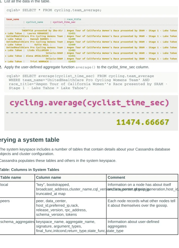
Create User-Defined Aggregate Function (UDA)
User-Defined Aggregates(UDAs) can be used to manipulate stored data across rows of data, returning a result that is further manipulated by a final function.Cassandra 2.2 and later allows users to define aggregate functions that can be applied to data stored in a table as part of a query result. The function must be created prior to its use in a SELECT statement and the query must only include the aggregate function itself, but no columns. The state function is called once for each row, and the value returned by the state function becomes the new state. After all rows are processed, the optional final function is executed with the last state value as its argument. Aggregation is performed by the coordinator.
The example shown computes the team average for race time for all the cyclists stored in the table. The race time is computed in seconds.
Procedure
• Create a state function, as a user-defined function (UDF), if needed. This function adds all the race times together and counts the number of entries.
cqlsh> CREATE OR REPLACE FUNCTION avgState ( state tuple<int,bigint>, val int ) CALLED ON NULL INPUT RETURNS tuple<int,bigint> LANGUAGE java AS 'if (val !=null) { state.setInt(0, state.getInt(0)+1); state.setLong(1, state.getLong(1)+val.intValue()); } return state;';
• Create a final function, as a user-defined function (UDF), if needed. This function computes the average of the values passed to it from the state function.
cqlsh> CREATE OR REPLACE FUNCTION avgFinal ( state tuple<int,bigint> ) CALLED ON NULL INPUT RETURNS double LANGUAGE java AS
'double r = 0; if (state.getInt(0) == 0) return null; r =
state.getLong(1); r/= state.getInt(0); return Double.valueOf(r);'; • Create the aggregate function using these two functions, and add an STYPE to define the data type
for the function. Different STYPEs will distinguish one function from another with the same name. An aggregate can be replaced with a different aggregate if OR REPLACE is used as shown in the examples above. Optionally, the IF NOT EXISTS keywords can be used to create the aggregate only if another aggregate with the same signature does not exist in the keyspace. OR REPLACE and IF NOT EXISTS cannot be used in the same command.
cqlsh> CREATE AGGREGATE IF NOT EXISTS average ( int )
SFUNC avgState STYPE tuple<int,bigint> FINALFUNC avgFinal INITCOND (0,0);
Inserting and updating data
How to insert data into a table with either regular or JSON data.Data can be inserted into tables using the INSERT command. With Cassandra 3.0, JSON data can be inserted.
Inserting simple data into a table
Inserting set data with the INSERT command.In a production database, inserting columns and column values programmatically is more practical than using cqlsh, but often, testing queries using this SQL-like shell is very convenient.
Insertion, update, and deletion operations on rows sharing the same partition key for a table are performed atomically and in isolation.
Procedure
• To insert simple data into the table cycling.cyclist_name, use the INSERT command. This example inserts a single record into the table.
cqlsh> INSERT INTO cycling.cyclist_name (id, lastname, firstname) VALUES (5b6962dd-3f90-4c93-8f61-eabfa4a803e2, 'VOS','Marianne');
• You can insert complex string constants using double dollar signs to enclose a string with quotes, backslashes, or other characters that would normally need to be escaped.
cqlsh> INSERT INTO cycling.calendar (race_id, race_start_date, race_end_date, race_name) VALUES
(201, '2015-02-18', '2015-02-22', $$Women's Tour of New Zealand$$);
Inserting and updating data into a set
How to insert or update data into a set.If a table specifies a set to hold data, then either INSERT or UPDATE is used to enter data.
Procedure
• Insert data into the set, enclosing values in curly brackets.
Set values must be unique, because no order is defined in a set internally.
cqlsh>INSERT INTO cycling.cyclist_career_teams (id,lastname,teams) VALUES (5b6962dd-3f90-4c93-8f61-eabfa4a803e2, 'VOS',
{ 'Rabobank-Liv Woman Cycling Team','Rabobank-Liv Giant','Rabobank Women Team','Nederland bloeit' } );
• Add an element to a set using the UPDATE command and the addition (+) operator. cqlsh> UPDATE cycling.cyclist_career_teams
SET teams = teams + {'Team DSB - Ballast Nedam'} WHERE id = 5b6962dd-3f90-4c93-8f61-eabfa4a803e2;
• Remove an element from a set using the subtraction (-) operator. cqlsh> UPDATE cycling.cyclist_career_teams
SET teams = teams - {'WOMBATS - Womens Mountain Bike & Tea Society'} WHERE id = 5b6962dd-3f90-4c93-8f61-eabfa4a803e2;
• Remove all elements from a set by using the UPDATE or DELETE statement.
A set, list, or map needs to have at least one element; otherwise, Cassandra cannot distinguish the set from a null value.
cqlsh> UPDATE cyclist.cyclist_career_teams SET teams = {} WHERE id = 5b6962dd-3f90-4c93-8f61-eabfa4a803e2;
DELETE teams FROM cycling.cyclist_career_teams WHERE id = 5b6962dd-3f90-4c93-8f61-eabfa4a803e2;
Inserting and updating data into a list
How to insert or update data into a list.If a table specifies a list to hold data, then either INSERT or UPDATE is used to enter data.
Procedure
• Insert data into the list, enclosing values in square brackets.
INSERT INTO cycling.upcoming_calendar (year, month, events) VALUES (2015, 06, ['Criterium du Dauphine','Tour de Suisse']);
• Use the UPDATE command to insert values into the list. Prepend an element to the list by enclosing it in square brackets and using the addition (+) operator.
cqlsh> UPDATE cycling.upcoming_calendar SET events = ['The Parx Casino Philly Cycling Classic'] + events WHERE year = 2015 AND month = 06; • Append an element to the list by switching the order of the new element data and the list name in the
UPDATE command.
cqlsh> UPDATE cycling.upcoming_calendar SET events = events + ['Tour de France Stage 10'] WHERE year = 2015 AND month = 06;
These update operations are implemented internally without any read-before-write. Appending and prepending a new element to the list writes only the new element.
• Add an element at a particular position using the list index position in square brackets.
cqlsh> UPDATE cycling.upcoming_calendar SET events[2] = 'Vuelta Ciclista a Venezuela' WHERE year = 2015 AND month = 06;
To add an element at a particular position, Cassandra reads the entire list, and then rewrites the part of the list that needs to be shifted to the new index positions. Consequently, adding an element at a particular position results in greater latency than appending or prefixing an element to a list.
• Remove an element from a list, use the DELETE command and the list index position in square brackets. For example, remove the event just placed in the list in the last step.
cqlsh> DELETE events[2] FROM cycling.upcoming_calendar WHERE year = 2015 AND month = 06;
The method of removing elements using an indexed position from a list requires an internal read. In addition, the client-side application could only discover the indexed position by reading the whole list
and finding the values to remove, adding additional latency to the operation. If another thread or client prepends elements to the list before the operation is done, incorrect data will be removed.
• Remove all elements having a particular value using the UPDATE command, the subtraction operator (-), and the list value in square brackets.
cqlsh> UPDATE cycling.upcoming_calendar SET events = events - ['Tour de France Stage 10'] WHERE year = 2015 AND month = 06;
Using the UPDATE command as shown in this example is recommended over the last example because it is safer and faster.
Inserting and updating data into a map
How to insert or update data into a map.If a table specifies a map to hold data, then either INSERT or UPDATE is used to enter data.
Procedure
• Set or replace map data, using the INSERT or UPDATE command, and enclosing the integer and text values in a map collection with curly brackets, separated by a colon.
cqlsh> INSERT INTO cycling.cyclist_teams (id, lastname, firstname, teams) VALUES (
5b6962dd-3f90-4c93-8f61-eabfa4a803e2, 'VOS',
'Marianne',
{2015 : 'Rabobank-Liv Woman Cycling Team', 2014 : 'Rabobank-Liv Woman Cycling Team', 2013 : 'Rabobank-Liv Giant',
2012 : 'Rabobank Women Team', 2011 : 'Nederland bloeit' }); Note: Using INSERT in this manner will replace the entire map.
• Use the UPDATE command to insert values into the map. Append an element to the map by enclosing the key-value pair in curly brackets and using the addition (+) operator.
cqlsh> UPDATE cycling.cyclist_teams SET teams = teams + {2009 : 'DSB Bank - Nederland bloeit'} WHERE id = 5b6962dd-3f90-4c93-8f61-eabfa4a803e2; • Set a specific element using the UPDATE command, enclosing the specific key of the element, an
integer, in square brackets, and using the equals operator to map the value assigned to the key. cqlsh> UPDATE cycling.cyclist_teams SET teams[2006] = 'Team DSB - Ballast Nedam' WHERE id = 5b6962dd-3f90-4c93-8f61-eabfa4a803e2;
• Delete an element from the map using the DELETE command and enclosing the specific key of the element in square brackets:
cqlsh> DELETE teams[2009] FROM cycling.cyclist_teams WHERE id=e7cd5752-bc0d-4157-a80f-7523add8dbcd;
• Alternatively, remove all elements having a particular value using the UPDATE command, the subtraction operator (-), and the map key values in curly brackets.
Inserting tuple data into a table
Tuples are used to group small amounts of data together that are then stored in a column.
Procedure
• Insert data into the table cycling.route which has tuple data. The tuple is enclosed in parentheses. This tuple has a tuple nested inside; nested parentheses are required for the inner tuple, then the outer tuple.
cqlsh> INSERT INTO cycling.route (race_id, race_name, point_id, lat_long) VALUES (500, '47th Tour du Pays de Vaud', 2, ('Champagne', (46.833, 6.65)));
• Insert data into the table cycling.nation_rank which has tuple data. The tuple is enclosed in parentheses. The tuple called info stores the rank, name, and point total of each cyclist.
cqlsh> INSERT INTO cycling.nation_rank (nation, info) VALUES ('Spain', (1,'Alejandro VALVERDE' , 9054));
• Insert data into the table popular which has tuple data. The tuple called cinfo stores the country name, cyclist name, and points total.
cqlsh> INSERT INTO cycling.popular (rank, cinfo) VALUES (4, ('Italy', 'Fabio ARU', 163));
Inserting data into a user-defined type (UDT)
How to insert or update data into a user-defined type (UDT).If a table specifies a user-defined type (UDT) to hold data, then either INSERT or UPDATE is used to enter data.
Procedure
1. Set or replace defined type data, using the INSERT or UPDATE command, and enclosing the user-defined type with curly brackets, separating each key-value pair in the user-user-defined type by a colon.
cqlsh> INSERT INTO cycling.cyclist_stats (id, lastname, basics) VALUES ( e7ae5cf3-d358-4d99-b900-85902fda9bb0,
'FRAME',
{ birthday : '1993-06-18', nationality : 'New Zealand', weight : null, height : null }
);
Note: Note the inclusion of null values for UDT elements that have no value. A value, whether null or otherwise, must be included for each element of the UDT.
2. Data can be inserted into a UDT that is nested in another column type. For example, a list of races, where the race name, date, and time are defined in a UDT has elements enclosed in curly brackets that are in turn enclosed in square brackets.
cqlsh> INSERT INTO cycling.cyclist_races (id, lastname, firstname, races) VALUES (
5b6962dd-3f90-4c93-8f61-eabfa4a803e2, 'VOS',
[ { race_title : 'Rabobank 7-Dorpenomloop Aalburg',race_date : '2015-05-09',race_time : '02:58:33' },
{ race_title : 'Ronde van Gelderland',race_date : '2015-04-19',race_time : '03:22:23' } ]
);
Note: The UDT nested in the list is frozen, so the entire list will be read when querying the table.
Inserting JSON data into a table
Inserting JSON data with the INSERT command for testing queries.In a production database, inserting columns and column values programmatically is more practical than using cqlsh, but often, testing queries using this SQL-like shell is very convenient. With Cassandra 2.2 and later, JSON data can be inserted. All values will be inserted as a string if they are not a number, but will be stored using the column data type. For example, the id below is inserted as a string, but is stored as a UUID. For more information, see What's New in Cassandra 2.2: JSON Support.
Procedure
• To insert JSON data, add JSON to the INSERT command.. Note the absence of the keyword VALUES and the list of columns that is present in other INSERT commands.
cqlsh> INSERT INTO cycling.cyclist_category JSON '{ "category" : "GC",
"points" : 780,
"id" : "829aa84a-4bba-411f-a4fb-38167a987cda", "lastname" : "SUTHERLAND" }';
• A null value will be entered if a defined column like lastname, is not inserted into a table using JSON format.
cqlsh> INSERT INTO cycling.cyclist_category JSON '{ "category" : "Sprint",
"points" : 700,
"id" : "829aa84a-4bba-411f-a4fb-38167a987cda" }';
Using lightweight transactions
INSERT and UPDATE statements that use the IF clause support lightweight transactions, also known as Compare and Set (CAS).INSERT and UPDATE statements using the IF clause support lightweight transactions, also known as Compare and Set (CAS). A common use for lightweight transactions is an insertion operation that must be unique, such as a cyclist's identification. Lightweight transactions should not be used casually, as the
It is important to note that using IF NOT EXISTS on an INSERT, the timestamp will be designated by the lightweight transaction, and USING TIMESTAMP is prohibited.
Procedure
• Insert a new cyclist with their id.
cqlsh> INSERT INTO cycling.cyclist_name (id, lastname, firstname)
VALUES (4647f6d3-7bd2-4085-8d6c-1229351b5498, 'KNETEMANN', 'Roxxane') IF NOT EXISTS;
• Perform a CAS operation against a row that does exist by adding the predicate for the operation at the end of the query. For example, reset Roxane Knetemann's firstname because of a spelling error.
cqlsh> UPDATE cycling.cyclist_name SET firstname = ‘Roxane’
WHERE id = 4647f6d3-7bd2-4085-8d6c-1229351b5498 IF firstname = ‘Roxxane’;
Expiring data with Time-To-Live
Data in a column, other than a counter column, can have an optional expiration period called TTL (time to live).Data in a column, other than a counter column, can have an optional expiration period called TTL (time to live). The client request specifies a TTL value, defined in seconds, for the data. TTL data is marked with a tombstone after the requested amount of time has expired. A tombstone exists for gc_grace_seconds. After data is marked with a tombstone, the data is automatically removed during the normal compaction and repair processes.
Use CQL to set the TTL for data.
If you want to change the TTL of expiring data, the data must be re-inserted with a new TTL. In Cassandra, the insertion of data is actually an insertion or update operation, depending on whether or not a previous version of the data exists.
TTL data has a precision of one second, as calculated on the server. Therefore, a very small TTL is not very useful. Moreover, the clocks on the servers must be synchronized; otherwise reduced precision will be observed because the expiration time is computed on the primary host that receives the initial insertion but is then interpreted by other hosts on the cluster.
Expiring data has an additional overhead of 8 bytes in memory and on disk (to record the TTL and expiration time) compared to standard data.