Efficient Autoscaling in the Cloud using Predictive Models for Workload Forecasting

Efficient Autoscaling in the Cloud using Predictive Models for Workload Forecasting

Nilabja Roy, Abhishek Dubey and Aniruddha Gokhale ∗_{Dept. of EECS, Vanderbilt University, Nashville, TN 37235, USA}

Email: {nilabjar,dabhishe,gokhale}@dre.vanderbilt.edu

Abstract—Large-scale component-based enterprise applica-tions that leverage Cloud resources expect Quality of Service (QoS) guarantees in accordance with service level agreements between the customer and service providers. In the con-text of Cloud computing, autoscaling mechanisms hold the promise of assuring QoS properties to the applications while simultaneously making efficient use of resources and keeping operational costs low for the service providers. Despite the perceived advantages of autoscaling, realizing the full potential of autoscaling is hard due to multiple challenges stemming from the need to precisely estimate resource usage in the face of significant variability in client workload patterns. This paper makes three contributions to overcome the general lack of effective techniques for workload forecasting and optimal resource allocation. First, it discusses the challenges involved in autoscaling in the cloud. Second, it develops a model-predictive algorithm for workload forecasting that is used for resource autoscaling. Finally, empirical results are provided that demonstrate that resources can be allocated and deallocated by our algorithm in a way that satisfies both the application QoS while keeping operational costs low.

Keywords-autoscaling; workload forecasting; predictive mod-els.

I. INTRODUCTION

Large enterprise software systems such as (e.g., eBay, Priceline, Amazon and Facebook), need to provide high assurance in terms of Quality of Service (QoS) metrics such as response times, high throughput, and service availability to their users. Without such assurances, service providers of these applications stand to lose their user base, and hence their revenues. Typically customers maintain Service Level Agreements (SLAs) with service providers for the QoS properties. Failure to comply with satisfying these QoS metrics leads to a major loss of revenue in the form of decreased user base [1].

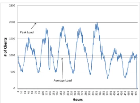
Catering to the SLA while still keeping costs low is challenging for such enterprise systems due primarily to the varying number of incoming customers to the system. For example, consider Figure 1 which depicts a real-world scenario wherein workload of the FIFA 1998 soccer world cup website in the number of incoming clients to such a website is highly varying depending upon a number of factors such as time of day, day of week and other seasonal factors. Such a workload is very typical of all commercial websites and planning capacity for such workload is not easy. Capacity could be planned for the average load as

shown in Figure 1 or for the peak load. Each approach has its disadvantages, however.

1000 1500 2000 2500 #ofClien ts PeakLoad 0 500 1 16 31 46 61 76 91 106 121 136 151 166 181 196 211 226 241 256 271 286 301 316 331 346 361 376 391 406 421 436 451 466 481 496 Hours Average Load

Figure 1. World Cup Soccer 1998 Workload

When planned for the average load, there is less cost incurred due to less hardware used but performance will be a problem when peak load occurs. Bad performance will dis-courage customers and revenue will be affected. On the other hand if capacity is planned for peak workload, resources will remain idle most of the time. Autoscaling supported in Cloud computing environments overcomes these challenges. Cloud computing providers such as Amazon EC2 provide access to hardware which can be allocated or deallocated at any time. Images of client software can be created before hand which can be loaded on to the machine. When not required, the same machines can be released. Machine usage costs on an hourly basis. Amazon EC2 provides an API which can be used to automate this process.

A problem with such a resource allocation scheme is the chance of thrashing where due to frequent variation of workload, machines can be added and released on every sample – a process that involves significant overhead as described in Section III. A desirable solution would require an ability to predict the incoming workload on the system and allocate resourcesa priori. This capability in turn will enable the application to be ready to handle the load increase when it actually occurs. A corollary requirement is the need to identify how many machines should actually be provi-sioned and started to handle the predicted load. For example, consider a situation where there areN number of machines already running and handling M customers for a given application. Suddenly, the number of customers increases toM + 100 and processor utilization also increases in the running nodes. Naturally, this situation requires increasing

the number of machines allocated, but how by how much is unknown. Anything less will provide degraded performance; anything more implies cost incurred by the customer for resources not actually used by the application.

In summary, autoscaling the resources in a cloud environ-ment is not an easy and straightforward task. Overcoming these challenges will require algorithms which take into account the following: (i) overheads related to state tran-sition when number of resources are changed, (ii) ability to accurately predict future workload, and (iii) compute the right number of resources required for the expected increase or decrease in workload. This paper describes a resource allocation algorithm based on model predictive techniques which allocates or deallocates machines to the application based upon optimizing the utility of the application over a limited prediction horizon.

The rest of the paper is organized as follows: Section II compares related research to our work; Section III described the challenges in workload prediction and relating it to autoscaling; Section IV describes our solution approach; Section V provides empirical evaluation of our algorithm; and finally Section VI provides concluding remarks.

II. RELATEDWORK

We have surveyed related work that investigates resource allocation and workload prediction, which are geared to-wards satisfying Cloud user requirements. We also focus on related work on optimizing resources, which is geared towards the Cloud provider. These dimensions of research are most appropriate for the work presented in this paper.

(1) Heuristics-based virtual machine allocation and

mi-gration: Urgaonkar et. al. [2] have used virtual machines

(VM) to implement dynamic provisioning of multi-tiered applications based on an underlying queuing model. For each physical host, however, only a single VM can be run. Wood et. al. [3] use a similar infrastructure as in [2]. They concentrate primarily on dynamic migration of VMs to support dynamic provisioning. They define a unique metric based on the consumption data of the three resources: CPU, network and memory to make the migration decision. Cunha et. al. [4] develop a comprehensive queuing model to model virtual servers. They assign each class of jobs in an application onto a virtual machine. They introduce a pricing model which gives rewards for throughput to be within SLA limits and penalty for throughput going above.

(2) Autonomic management of virtual computing

envi-ronment using control-theoretic approaches: Padala et.

al. [5] provide a control-theoretic solution where each tier of the application is executed on each virtual machine. Authors carry out black box profiling of the applications and build an approximated model which relates performance attributes such as response time to the fraction of processor allocated to the virtual machine running the application. Wang et. al. [6] describe a two-level control architecture for a

virtualized environment. A load balancing controller ensures that the virtual machines are all load-balanced and the response time of the applications in all the virtual machines are the same. Moreno et. al. [7] recommend an architecture for elastic management of cluster-based services. It consists of a virtualized infrastructure layer that works with a VM manager and a cloud service provider. This approach helps in autoscaling resources with the least amount of perturbations to the user. Waheed et. al. [8] propose a reactive algorithm to allocate extra resources to a cluster farm when workload increases, while Yang et. al [9] propose a profile-based approach to the problem of just-in-time scalability in a cloud environment.

Limitations in related work: The work in [2] and [3] do

not relate the placement mechanism to an overall utility value to the Cloud provider. They attempt at increasing the throughput of the application only. The applications considered do not have multiple classes, which is unrealistic. Although the work in [4] has a good utility model of the data center and multiple classes are considered, they assign every class onto a single virtual machine, which may not be cost-effective in a situation where an application has numerous classes. Although the utilization model given in [10] maps resource utilization to application utility, finding such a mapping is difficult [11]. Instead it is straightforward to relate throughput with utility and then map resource allocation to throughput. Such an approach, however, will need a robust analytical model for relating throughput with resource allocation.

III. CHALLENGES TOELASTICRESOURCE

PROVISIONING INCLOUDENVIRONMENTS

This section discusses the challenges to realizing elas-tic resource provisioning in large-scale component-based systems. Many of the challenges that are faced in elastic resource provisioning using autoscaling can be highlighted from the workload pattern in Figure 1.

A. Challenge 1: Workload Forecasting

The autoscaling strategy in a cloud environment will involve the acquiring and release of resources as workload imposed by the application changes with time. Both these tasks require programming to an API. Releasing resources is easy, however, acquiring resources incurs performance overheads stemming due to the following reasons. First, there is a need to make a call on the Cloud API which starts the acquisition process. The machines will then be needed to boot up with the specified image, the application need to be started, and there also might be the need for state update. Thus, it is desirable if the resources can be acquired earlier than the time when workload actually increases. This outcome can be possible only if the future workload can be predicted, possibly using historical data. Section IV-A shows

our solution to predict workload in the next interval by using the workload patterns up to the current interval.

B. Challenge 2: Identify Resource Requirement for Incom-ing Load

Figure 1 plots the number of customers who use the system every hour. Since the number of customers vary every hour, the number of resources required also varies. The required number of resources is a function of the number of customers, the nature of the application, and also the type of calls that each customer makes on the application. The resources required need to be estimated properly so that they can be provisioned within the cloud infrastructure. The resource estimation also needs to be very accurate. If it is not accurate then there is the potential of under-or over-provisioning of resources, each of which has its pitfalls. Section IV-B describes our solution to determine the accurate number of resources needed.

C. Challenge 3: Resource Allocation while Optimizing Mul-tiple Cost Factors

To optimize resource usage and/or minimize idle re-sources, an ideal solution is to define a time interval and change resources as many times as possible as workload changes. In the limit this interval could be made infinites-imally small and resources are changed continuously in accordance with the change in load, assuming we can always at least over estimate the load. This extreme will obviously ensure that the optimum number of resources are always used. Obviously, such as scheme is not possible since chang-ing resources is not spontaneous. Challenge 1 highlights the overhead in allocating a resource. Thus, scaling up or down resources also involves cost and needs to be optimized. Section IV-C describes our approach to avoid thrashing and system instability by planning a resource allocation strategy based on a limited future horizon.

IV. AUTO-SCALINGRESOURCES USINGLOOK-AHEAD

OPTIMIZATIONS

Control theory offers a promising methodology to address the challenges described in Section III. It allows systemati-cally solving a general class of dynamic resource provision-ing problems usprovision-ing the same basic control concepts, and to verify the feasibility of a control scheme before deployment on the actual system. In more complex control problems a pre-specified plan called the feedback map becomes in-flexible and does not adapt well to constantly changing operating conditions. Therefore, researchers have studied the use of more advanced state-space methods adapted from model predictive control [12] and limited look-ahead supervisory control [13] to manage such applications [14]– [16]. These methods offer a natural framework to accom-modate the above-described system characteristics, and take

into account multi-objective non-linear cost functions, fi-nite control input sets and dynamic operating constraints while optimizing application performance. The autonomic approach proposed in [16], [17] describes a hierarchical control based framework to manage the high level goals for a distributed computing system by continuous observation of the underlying system performance. The key differences between these previous works and our work is in the nature of the performance models.

The autoscaling algorithm presented in this paper does not use a reactive strategy. Instead it provides a predictive solution leveraging concepts proposed by Sherif, et. al. [18], [19], which is applicable to systems that exhibit a hybrid behavior comprising both discrete-event and continuous dy-namics and have a possibly large but finite set of control options. Formally, it has been shown before in the literature that dynamics of such systems can be captured using the model of switching hybrid systems. It is known that for such systems a multi objective control problem can be solved by using a limited look-ahead controller algorithm [18], [19], which is a type of model predictive control. This is done by selecting actions that optimize system behavior over a limited prediction horizon.

The rest of this section describes our approach and shows how we resolve the three challenges described in Section III. A. Workload Prediction

To apply model predictive control ideas to the problem discussed in this paper we predict the workload on the appli-cation and estimate the system behavior over the prediction horizon using a performance model. The optimization of the system behavior is carried on by minimizing the cost incurred to the application. This cost is a combination of various factors such as cost of SLA violations, leasing cost of resources and a cost associated with the changes to the configuration. The advantage of such a method is that it can be applied to various performance management problems from systems with simple linear dynamics to complex ones. The performance model can also be varied and corrected with system dynamics as conditions in the environment like workload variation or faults in the system change.

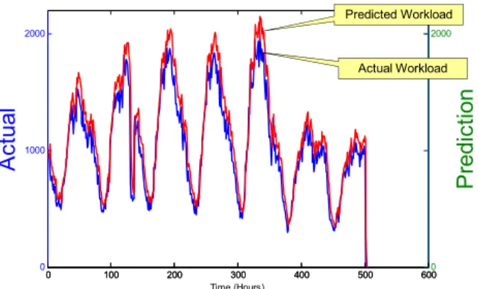
In our strategy, workload prediction is needed to estimate the incoming workload of the system for future time periods. Thankfully a number of techniques already exist in literature that can be applied for forecasting the traffic incident on a service. We used a second order autoregressive moving average method (ARMA) filter for the workload shown in Figure 1. The equation for the filter used is given by

λ(t+1) =β×λ(t)+γ×λ(t−1)+(1−(β+γ))(λ(t−2)) (1) The value for the variablesβandγare given by the values 0.8 and 0.15, respectively. Figure 2 shows the predicted workload compared to the actual workload.

0 100 200 300 400 500 600 0 1000 2000

Ac

tu

a

l

P

redi

c

ti

on

Figure 2. Predicted vs. actual workload shown over a single look-ahead horizon.

B. Performance Model

The next challenge we resolve is identifying resource requirements for the predicted workload. The right number of resources is the one that will provide the desired response times (or other performance metrics) of the applications. For the above look-ahead framework we focus on response times of the application under different hardware configurations. The workload used in this work is the number of users currently in the system. It also depends upon what each user does. For example, some users could be browsing while some users could be entering data in a form. In our prior work [20] we have used Customer Behavior Modeling Graphs (CBMG) to model the overall behavior of customers. A CBMG is built from a log of previous customer behavior and computes the probability of a typical user to visit each page. Using this information, we can calculate the number of visits to a single page from the total number of customers in the system. The number of visits to each page helps in calculating the average load on each page.

Our prior work also developed analytical models to ac-curately estimate response times, which are used in Algo-rithm 1. This algoAlgo-rithm accepts the amount of workload given by a vector of client populations, each member representing the number of clients in each job class. The number of machines provided, the service demand of the components and the think time for clients is also given as input. Algorithm 1 initially creates a default placement strategy whereby it places each tier of the application onto a particular machine. Purposefully we start off with a low number of machines (2) and gradually increase the load to identify the right number of resources required. This approach helps to avoid a situation where we need to reduce the number of machines (M − 1) on each iteration, the algorithm makes a call onto the Mean Value Analysis (MVA) algorithm. The MVA returns the utilization of each tier which can be used to find the bottleneck machine (the machine with the highest utilization). The tier present in that

machine is then replicated and placed in a new machine which is introduced in that iteration. In this manner, the iteration continues until the total number of machines equal the given maximum machines.

Algorithm 1:Response Time Analysis (RTA)

Input:

LdPredicted Workload

HwTotal Machines available

SDService Demand for the job classes

ZThink Time

Output:

Response TimeR←Vector of response times for all job classes

1begin

2 // start with one machine per tier (2 in this case)

3 M = 2;

4 whileM <=Hwdo

5 // Get response time and server utilization by running MVA on analytical model presented in [20]

6 [R, U] = MVA (SD, Ld, Z);

7 i = maxUtil (U);// Get the index of the bottleneck tier

8 // Add a machine and replicate tier i on it to balance the load

9 M = M + 1

10 M←i

C. Optimizing Resource Provisioning

To optimize resource usage and minimize idle resources, the best way would be to define a time interval and change resources as many times as possible as workload changes. In the limit this interval could be made infinitesimally small and resources are changed continuously, however, as noted earlier such an extreme solution is not feasible. The intuition therefore is to identify the right number of time intervals in which to make these adjustments with the requirement that the time interval is neither too small nor too large. Our solution works on the principles of receding horizon control also known as look-ahead optimization [19].

This form of controller, iteratively solves an optimiza-tion problem, Costopt _{starting from t0, over a predefined}

horizon (t = 1...N) taking into account current and future constraints. Once a feasible sequence is found, only the first input in the sequence is applied and the rest are discarded. Effectively, the optimization search results in the construction of a tree with branching factorK and N+ 1 levels. Here K is the total number of finite input choices. Formally, at timet0, given state xt0

Costopt_=min{Cost({x

t},{ut})} {} denotes a set

xt+1=f(xt, ut), t=t0,· · · , tN−1

ut ∈Ufinite input choices

XN is the set of final goal states

Cost({xt},{ut}) = (

t=t0+N−1

t=t0+1

J(x(t), u(t)) where J is a utility function A sequence {u_t} = {u0,· · ·, uN−1} and{xt} = {x0,· · ·, xN−1} are the feasible input sequence and the

resulting states that trace a path from the root to the lead node in this search tree such that the net cost across the sum of all branches is minimum and the leaf node is closest to the final destination state.

Given that this method needs finite input choices, we use a finite range of machines that can be increased, decreased, or kept the same. The next challenge is the choice of the look-ahead period. A small look-ahead period will neglect trends, while a very large period will increase computational complexity and lead to a larger prediction error, which will yield any control decision ineffective. Thus, the number of look-ahead periods need to balance out the different tradeoffs.

To implement the receding horizon control algorithm in our setting we make the following observations. The actual algorithm is not described here because the implementation requires recursive data structures and is difficult to describe in the limited space available.

Number of Look-ahead steps N

SLA response time bound R∗

State Variable Machines Used,M

Control Options u, range of change

Workload W

Service Demand for the job classes SD

Thinktime Z

Cost Function Equation 5

State Advance Function Equation 2

Our algorithm uses the receding horizon control and iterates over the number of look-ahead steps and calculates the cumulative costs. For every future time step, it computes the cost of selecting each possible resource allocation. To compute the cost of a particular allocation, it uses Algo-rithm 1 to compute the estimated response time for that particular machine configuration. Once the response time is calculated, it is used to calculate the cost of the allocation which is a combination of how far the estimated response time is from the SLA bounds, cost of leasing additional machines and also a cost of re-configuration.

Wt=β×Wt−1+γ×Wt−2+ (1−β−γ)×Wt−3 (2)

Mt=Mt−1+ut (3)

Rt =ResponseT imeAnalysis(Wt, Mt, SD, Z) (4)

The cost of reconfiguration is computed based on the number of machines that need to updated. Obviously re-configuration will incur some costs and thus the algorithm will try to reduce the amount of reconfiguration. Each of these cost components will have weights attached to them which may be varied depending on the type of application and its requirements. Applications are required to specify which factors are more important to them, and our auto-scaling algorithm will honor these specifications in making the decisions. Section V illustrates different behaviors re-sulting from different choices for these weights.

V. EXPERIMENTALEVALUATION

This section presents results evaluating our look-ahead algorithm. We first show how the algorithm determines the number of resources to be allocated in a just-in-time manner so that the overall cost is minimized. Next, the effects of different cost weightage is studied.1 _{This study is important}

since different applications may impose different weightage combinations. The data used in this study is acquired from the 1998 soccer world cup web site shown in Figure 1. We use the number of customers visiting that site as an indication of the amount of workload that typically can be experienced by such a globally popular topic.

A. Just-in-time Resource Allocation

To evaluate the strength of our just-in-time resource allocation, we have used a cost function shown in Equation 5 comprising the three components. Recall that the three com-ponents of the cost function refer individually to the penalty for violation of SLA bounds, cost of leasing a machine, and cost of reconfiguring the application when machines are either leased or released. Each of these components has a weight attached to it and the system can be made to always minimize a certain component by increasing the attached weight to it to an arbitrary high value. Table I describes the components of the cost function.

Cost=Wr×(Rsla−R)+Wc×Mk+Wf×(Mk−Mk−1)

(5)

Table I

COMPONENTS OFCOSTFUNCTION

Component Description Unit

Wr Penalty for SLA violation $/sec

Wc Cost of Leasing a Machine per hour $/machine

Wf Cost of reconfiguring application $/machine

Rsla SLA given response time sec

R Maximum response time of application sec

Mk Number of machines used in thekthinterval Numeric

Mk−1 Number of machines used in thek−1th_{interval Numeric}

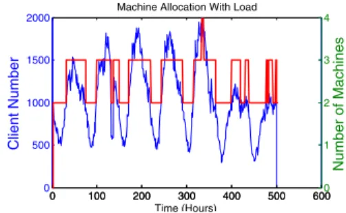
For this experiment, the weights on each component of the cost function is the same, which means all factors are equally important. Figure 3 shows how the look-ahead algorithm determines changes in the resources required as the incoming load changes. The computation is done on the basis of predicted workload which is done with the help of the ARMA filter given in Equation 1. Figure 3 clearly shows that the base resources required are2machines and it increases to 3or4when the load is increased. The prediction of the look-ahead algorithm based on a selected number of time intervals closely matches the incoming load. It prescribes resource increase whenever there is high load and less resources when there is less load. Thus Figure 3 shows the effectiveness of

1_{Due to space restrictions we are unable to showcase a variety of different} configurations.

the look-ahead algorithm and how it can save cost while also assuring that the performance of the application is assured.

0 100 200 300 400 500 600 0 500 1000 1500 2000 Client Number Time (Hours) Machine Allocation With Load

0 100 200 300 400 500 6000 1 2 3 4 Number of Machines

Figure 3. Just-in-time Resource Allocation with Changing Load

B. Resource Usage under Different Cost Priorities

The results in this section demonstrate the alloca-tion/deallocation of resources stemming from using different cost ratios among the three competing factors in the cost function of Equation 5. The resource allocation determined by our algorithm in the different time intervals will depend upon the weights assigned to the various components of the cost function. The rest of the section studies the different trends of resource allocation and how they are influenced by the varying weights of the cost function.

1) SLA violation against Resource Cost: We first show the results when considering the effect of SLA violation against cost of resources,i.e., the ratio of the cost of SLA violation against the cost of machines are varied while the application reconfiguration cost is assumed to be zero. We assume that the application can be easily reconfigured with varying machines. The ratio of SLA penalty to machine cost is varied from 4 : 1(which means SLA violation is higher priority than cost of the machine) to 1 : 13 (which means that the machine cost is higher priority than SLA violation). Figures 4, 5 and 6 show how the resources are allocated every hour over the entire time period. The corresponding cost values are also shown in the bottom graph for each of these figures. The intervals over which there are SLA violations are also shown. The algorithm always tries to keep the cost to a minimum. It is seen that there is signifi-cant difference in resource allocation between the different configurations. An application with high SLA violation penalty has stronger performance assurance whereas one with low SLA penalty has lesser performance assurance. The priorities of the application determine the difference in resource allocation. For a low performance assurance and high machine cost, the number of machines used is only 2 over the entire time interval. The cost of machines exceeds the cost of SLA violations and such a configuration will have to tolerate a number of SLA violations (Figure 4).

Contrary to this configuration, for an application that can tolerate some SLA violations (medium SLA violations), Figure 5 shows how there are many intervals in which 3

0 100 200 300 400 500 600 0 1000 2000 C lie nt N u m b er

Machine Allocation With Load

0 100 200 300 400 500 6000 2 4 N u mber of Mac h in es 0 100 200 300 400 500 600 0 10 20 Co s t Time (Hours) Cost & SLA Violation

0 100 200 300 400 500 6000 0.5 1 SL A Vi o la ti o n Number of Machines Cost of 3 Machines SLA Violation Cost slowly increases

Figure 4. Resource Allocation for Low SLA Violation Cost and High Machine Cost 0 100 200 300 400 500 600 0 1000 2000 C lie nt N u m b er

Machine Allocation With Load

0 100 200 300 400 500 6000 2 4 N u mber of Mac h in es 0 100 200 300 400 500 600 0 10 20 Co s t Time (Hours) Cost & SLA Violation

0 100 200 300 400 500 6000 0.5 1 SL A Vi o la ti o n Number of Machines Cost of 3 Machines SLA Violation Cost slowly increases

Figure 5. Resource Allocation for Medium SLA Violation Cost

machines are used. This balances the cost of machines and cost of SLA violations. For the highly assured application of Figure 6, there is much variation in resource usages with a number of intervals having3machines and also some having 4machines. Here the priority is in assuring performance and the cost of machines is much lower.

Finally, Figure 7 shows the distribution of number of machines required for a variety of systems ranging from highly assured systems (ratio of SLA violation penalty to machine cost being 4 : 1) to very weakly assured systems (ratio of SLA violation penalty to machine cost being > 1 : 13). In this figure, each point on the X-axis is a ratio of cost of SLA violation to the cost of machine. The Y-axis plots the number of intervals in which each type of

machine is used. For example, for the point corresponding to cost ratio of 1:4, 359 intervals use 2 machines and the other 143 intervals use 3 machines. The ratio of SLA violation cost to machine cost increases as we move further down the X-axis. The figure shows the use of more3machines than2 machines as we move to the right. This outcome is because the relative cost of machines decreases to the right and the penalty of SLA violation increases.

200 300 400 500 600 M achineDis tribution 0 100 1:13 1:12 1:11 1:10 1:9 1:8 1:7 1:6 1:5 1:4 1:3 1:2 1:1 2:1 3:1 4:1 M CostRatio SLAViolation:Machine 2Machines 3Machines 4Machines

Figure 7. Resource Allocation for Variety of Systems

2) Including the Cost of Reconfiguration: Figure 6 showed how resource allocation is done when there is high SLA violation cost compared to machine cost. For this configuration, in every interval, the mean response time is below the SLA bound and the machines are allocated whenever they are needed. A machine is released again since there is cost of machine but only making sure that the SLA is maintained. When there is a cost of reconfiguration intro-duced, the algorithm will resist the changing of resources. This phenomenon can be related to inertia in physical bodies. Inertia resists changes to its current physical condition such as a body in rest resists movement while a body in motion resists slowing down. Thus the cost of reconfiguration will similarly resist the dynamic nature of resource allocation.

Higher this cost, higher will be its resistance to the changes. This cost is expressed as the third component of Equation 5. The weight Wf represents the level of inertia

and it is multiplied by the change level which is the number of machines allocated or released. Initially when a small amount of reconfiguration cost is introduced, it does not effect much as shown in Figure 8. The resource allocation is similar to Figure 6. There are small deviations, where the spikes in resource changes are a little wider in Figure 8 than in Figure 6. This is due to the inertia in change introduced due to some cost associated with change.

The effect of the cost of reconfiguration is more pro-nounced when it is prioritized slightly higher. Figure 9 shows a distinct change in resource allocation over the hourly intervals compared to Figures 6 or 8. In Figure 9, the number of machines increases to 3at around the40th hour and remains steady. Somewhere around the 350th _{hour it}

increases to4machines since the workload increased at that

0 100 200 300 400 500 600 0 500 1000 1500 2000 Clie n t Nu m b e

r Machine Allocation With Load

0 100 200 300 400 500 6000 1 2 3 4 N u mber of Mac h in es 0 100 200 300 400 500 600 0 2 4 6 8 10 Co st Time (Hours) Cost & SLA Violation

0 100 200 300 400 500 6000 0.2 0.4 0.6 0.8 1 SL A Vi o la ti o n Number of Machines Cost SLA Violation

Cost SLA Violation

Figure 8. High SLA violation with Low Reconfiguration cost

time. Subsequent to that, the workload decreased but the ma-chines were never released since the cost of reconfiguration is considered much higher compared to the cost of machines. The changes of the machines around40and350hours was warranted because of the high SLA violation cost and the machines were never released even though the workload lessened since the cost of reconfiguration was higher.

0 100 200 300 400 500 600 0 500 1000 1500 2000 Clie n t Nu m b e

r Machine Allocation With Load

0 100 200 300 400 500 6000 1 2 3 4 N u mber of Mac h in es 0 100 200 300 400 500 600 0 5 10 Co st Time (Hours) Cost & SLA Violation

0 100 200 300 400 500 600-1 0 1 SL A Vi o la ti o n Number of Machines Cost No SLA Violation

Reconfiguration Cost + Machine Cost

Figure 9. High SLA violation with Medium Reconfiguration cost

0 100 200 300 400 500 600 0 1000 2000 Clie n t Nu m b e

r Machine Allocation With Load

0 100 200 300 400 500 6000 2 4 N u mber of Mac h in es 0 100 200 300 400 500 600 0 10 Co st Time (Hours) Cost & SLA Violation

0 100 200 300 400 500 600-1 0 1 SL A Vi o la ti o n Number of Machines Cost No SLA Violation Reconfiguration Cost + Machine Cost

Figure 10. High SLA violation with High Reconfiguration cost

This behavior of resisting change is further pronounced in Figure 10 where there is even higher cost of reconfiguration. Here again there is an increase of machines to3at around the 40hour mark and the machine is never released. The change to4 machines which was seen in Figure 9 does not occur here because the cost of reconfiguration is much higher that the cost of SLA violation. Thus even though there is SLA

violation, it is only of a short duration (the peak workload around 350 hour) and is of lesser cost than the cost of changing resources. That the SLA violation near 300 hour was of a short duration can be understood from Figure 8 where there is a very short spike of machine allocation to4 around that time. When the cost of reconfiguration becomes high, the look-ahead algorithm decides not to expend in the extra cost of reconfiguration to cover up that short SLA violation.

VI. CONCLUSION

Autoscaling of resources helps Cloud service providers operating modern day data centers to support maximal num-ber of customers while assuring customer QoS requirements in accordance with service level agreements, and keeping cost of using resources low for customers. However, current autoscaling mechanisms require user input and programming of APIs to adjust resources as workloads change. Reactive scaling of resources imposes performance overheads while also making the programming of Cloud infrastructure te-dious. To address these problems, this paper describes a look-ahead resource allocation algorithm based on model-predictive control which predicts future workload based on a limited horizon and adjusts resources allocated to users ahead-of-time. Empirical results evaluating our approach shows significant benefits both to Cloud users and providers. The work presented demonstrates the feasibility of our approach in the context of small number of machines used. Our future work will explore the scalability of our algorithms in the context of modern day workloads and large number of resources, which are typical of contemporary applications.

ACKNOWLEDGMENTS

This work was supported in part by NSF CNS Award #0915976 and AFRL GUTS. Any opinions, findings, and conclusions or recommendations expressed in this material are those of the author(s) and do not necessarily reflect the views of the National Science Foundation or AFRL.

REFERENCES

[1] M. Armbrust, A. Fox, R. Griffith, A. Joseph, R. Katz, A. Konwinski, G. Lee, D. Patterson, A. Rabkin, I. Stoica, and M. Zaharia, “A View of Cloud Computing,”Communications of the ACM, vol. 53, no. 4, pp. 50–58, 2010.

[2] B. Urgaonkar, P. Shenoy, A. Chandra, P. Goyal, and T. Wood, “Agile dynamic provisioning of multi-tier internet applica-tions,” ACM Trans. Auton. Adapt. Syst., vol. 3, no. 1, pp. 1–39, 2008.

[3] T. Wood, P. J. Shenoy, A. Venkataramani, and M. S. Yousif, “Black-box and gray-box strategies for virtual machine mi-gration,” inNSDI, 2007.

[4] S. Cunha, J. M. Almeida, V. Almeida, and M. Santos, “Self-adaptive capacity management for multi-tier virtualized environments,” inIntegrated Network Management, 2007, pp. 129–138.

[5] P. Padala, K. Shin, X. Zhu, M. Uysal, Z. Wang, S. Singhal, A. Merchant, and K. Salem, “Adaptive control of virtualized resources in utility computing environments,”ACM SIGOPS Operating Systems Review, vol. 41, no. 3, p. 302, 2007.

[6] Y. Wang, X. Wang, M. Chen, and X. Zhu, “Power-efficient response time guarantees for virtualized enterprise servers,” in RTSS ’08: Proceedings of the 2008 Real-Time Systems Symposium. Washington, DC, USA: IEEE Computer Society, 2008, pp. 303–312.

[7] R. Moreno-Vozmediano, R. S. Montero, and I. M. Llorente, “Elastic management of cluster-based services in the cloud,” inACDC ’09: Proceedings of the 1st workshop on Automated control for datacenters and clouds. New York, NY, USA: ACM, 2009, pp. 19–24.

[8] W. Iqbal, M. Dailey, and D. Carrera, “Sla-driven adaptive re-source management for web applications on a heterogeneous compute cloud,” inCloud Computing, ser. Lecture Notes in Computer Science, M. Jaatun, G. Zhao, and C. Rong, Eds. Springer Berlin / Heidelberg, 2009, vol. 5931, pp. 243–253. [9] Y. Jie, Q. Jie, and L. Ying, “A profile-based approach to just-in-time scalability for cloud applications,” sep. 2009, pp. 9 –16.

[10] M. Cardosa, M. R. Korupolu, and A. Singh, “Shares and utilities based power consolidation in virtualized server en-vironments,” in IM’09: Proceedings of the 11th IFIP/IEEE international conference on Symposium on Integrated Net-work Management. Piscataway, NJ, USA: IEEE Press, 2009, pp. 327–334.

[11] G. Khanna, K. Beaty, G. Kar, and A. Kochut, “Application performance management in virtualized server environments,” in 10th IEEE/IFIP Network Operations and Management Symposium, 2006 (NOMS 2006), 2006, pp. 373–381. [12] J. M. Maciejowski,Predictive Control with Constraints.

Lon-don: Prentice Hall, 2002.

[13] S. L. Chung, S. Lafortune, and F. Lin, “Limited lookahead policies in supervisory control of discrete event systems,”

IEEE Trans. Autom. Control, vol. 37, no. 12, pp. 1921–1935, Dec. 1992.

[14] S. Abdelwahed, S. Neema, J. Loyall, and R. Shapiro, “A hybrid control design for QoS management,” inProc. IEEE Real-Time Syst. Symp. (RTSS), 2003, pp. 366–369.

[15] S. Abdelwahed, N. Kandasamy, and S. Neema, “Online control for self-management in computing systems,” inProc. RTAS, 2004, pp. 365–375.

[16] N. Kandasamy, S. Abdelwahed, and M. Khandekar, “A hier-archical optimization framework for autonomic performance management of distributed computing systems,” inProc. 26th IEEE Int’l Conf. Distributed Computing Systems (ICDCS), 2006.

[17] D. Kusic, N. Kandasamy, and G. Jiang, “Approximation mod-eling for the online performance management of distributed computing systems,” inICAC ’07: Proceedings of the Fourth International Conference on Autonomic Computing, 2007, p. 23.

[18] S. Abdelwahed, J. Bai, R. Su, and N. Kandasamy, “On the application of predictive control techniques for adaptive

performance management of computing systems,” Network

and Service Management, IEEE Transactions on, vol. 6, no. 4, pp. 212 –225, dec. 2009.

[19] S. Abdelwahed, N. Kandasamy, and S. Neema, “A control-based framework for self-managing distributed computing systems,” in WOSS ’04: Proceedings of the 1st ACM SIG-SOFT workshop on Self-managed systems. New York, NY, USA: ACM, 2004, pp. 3–7.

[20] N. Roy, A. Dubey, A. Gokhale, and L. Dowdy, “A Capacity Planning Process for Performance Assurance of

Component-based Distributed Systems,” in Proceedings

of the 2nd ACM/SPEC International Conference on Performance Engineering (ICPE 2011). Karlsruhe, Germany: ACM/SPEC, Mar. 2011, pp. 259–270. [Online]. Available: http://doi.acm.org/10.1145/1958746.1958784