A Hybrid Evolutionary Algorithm for
Heterogeneous Fleet Vehicle Routing
Problems with Time Windows
Çağri Koç
Tolga Bektaş
Ola Jabali
Gilbert Laporte
March 2014
CIRRELT-2014-16
Çağri Koç
, Tolga Bektaş
, Ola Jabali
, Gilbert Laporte
1 Interuniversity Research Centre on Enterprise Networks, Logistics and Transportation (CIRRELT) 2 School of Management,Centre for Operational Research, Management Science and Information
systems (CORMSIS), University of Southampton, Southampton, SO17 1BJ, United Kingdom
3 Department of Logistics and Operations Management, HEC Montréal, 3000 Côte-Sainte-Catherine,
Montréal, Canada H3T 2A7
4 Department of Management Sciences, HEC Montréal, 3000 chemin de la Côte-Sainte-Catherine,
Montréal, Canada H3T 2A7
Abstract
.
This paper presents a hybrid evolutionary algorithm (HEA) to solve
heterogeneous fleet vehicle routing problems with time windows. There are two main
types of such problems, namely the Fleet Size and Mix Vehicle Routing Problem with
Time Windows (F) and the Heterogeneous Fixed Fleet Vehicle Routing Problem with Time
Windows (H), where the latter, in contrast to the former, assumes a limited availability of
vehicles. The main objective is to minimize the fixed vehicle cost and the distribution cost,
where the latter can be defined with respect to en-route time (T) or distance (D). The
proposed algorithm is able to solve the four variants of heterogeneous fleet routing
problem, called FT, FD, HT and HD, where the last variant is new. The HEA successfully
combines several metaheuristics and offers a number of new advanced efficient
procedures tailored to handle the heterogeneous fleet dimension. Extensive computational
experiments on benchmark instances have shown that the HEA is highly effective on FT,
FD and HT. In particular, 149 of the 360 best known solution values for the three
previously studied variants have been retrieved or improved within reasonable
computational times. New benchmark results on HD are also presented.
Keywords: Vehicle routing, time windows, heterogeneous fleet, genetic algorithm,
neighborhood search.
Acknowledgements. The authors gratefully acknowledge funding provided by the
Southampton Management School at the University of Southampton and by the Natural
Sciences and Engineering Research Council of Canada (NSERC) under grants 39682-10
and 436014-2013.
Results and views expressed in this publication are the sole responsibility of the authors and do not necessarily reflect those of CIRRELT.
Les résultats et opinions contenus dans cette publication ne reflètent pas nécessairement la position du CIRRELT et n'engagent pas sa responsabilité.
_____________________________ * Corresponding author: [email protected]
1.
Introduction
In heterogeneous fleet vehicle routing problems with time windows, one considers a fleet of vehicles with various capacities and vehicle-related costs, as well as a set of customers with known demands and time windows. These problems consist of determining a set of vehicle routes such that each customer is visited exactly once by a vehicle within prespecified time window, all vehicles start and end their routes at a depot, and the load of each vehicle does not exceed its capacity. There are two main categories of such problems, namely the Fleet Size and Mix Vehicle Routing Problem with Time Windows (F) and the Heterogeneous Fixed Fleet Vehicle Routing Problem with Time Windows (H). In category F, there is no limit in the number of available vehicles of each type, whereas such a limit exists in category H. Two measures are used to compute the total cost to be minimized. The first is based on the en-route time (T), which is the sum of the fixed vehicle cost and the trip duration without the service time. In this case, service times are only used to check feasibility and for performing adjustments to the departure time from the depot in order to minimize pre-service waiting times. The second cost measure is based ondistance (D) and consists of the fixed vehicle cost and the distance traveled by the vehicle, as is the case in the standard vehicle routing problem with time windows (VRPTW) (Solomon 1987).
We differentiate between four variants defined with respect to the problem category and to the way in which the objective function is defined, namely FT, FD, HT and HD. The first variant is FT, described by Liu and Shen (1999b) and the second is FD, introduced by Br¨aysy et al. (2008). The third variant HT was defined and solved by Paraskevopoulos et al. (2008). Finally, HD is a new variant which we introduce in this paper.
Several versions of these problems without time windows arise in distribution problems such as grocery store deliveries and mail collection, and have, to a large extent, been addressed in the vehicle routing literature. Hoff et al. (2010) and Belfiore and Yoshizaki (2009) describe several industrial aspects and practical applications of these problems. The most studied versions are the fleet size and mix vehicle routing problem, described by Golden et al. (1984), which considers an unlimited heterogeneous fleet, and the heterogeneous fixed fleet vehicle routing problem, proposed by Taillard (1999). For further details, the reader is referred to the surveys of Baldacci et al. (2008) and of Baldacci and Mingozzi (2009).
The FT variant has several extensions, e.g., multiple depots (Dondo et al. 2007, Bettinelli et al. 2011), overloads (Kritikos and Ioannou 2013), and split deliveries (Belfiore and Yoshizaki 2009, 2013). There exist several exact algorithms for the capacitated vehicle routing problem (VRP) (Toth and Vigo 2002, Baldacci et al. 2010), and for the heterogeneous VRP (Baldacci and Mingozzi 2009). However, to the best of our knowledge, no exact algorithm has been proposed for the
heterogeneous VRP with time windows, i.e., FT, FD and HT. The existing heuristic algorithms for these three variants are briefly described below.
Liu and Shen (1999b) proposed a heuristic for FT which starts by determining an initial solution through an adaptation of the Clarke and Wright (1964) savings algorithm, previously presented by Golden et al. (1984). The second stage improves the initial solution by moving customers by means of parallel insertions. The algorithm was tested on a set of 168 benchmark instances derived from the set of Solomon (1987) for the VRPTW. Dullaert et al. (2002) described a sequential construction algorithm for FT, which is an extension of the insertion heuristic of Golden et al. (1984). Dell’Amico et al. (2007) described a multi-start parallel regret construction heuristic for FT, which is embedded into a ruin and recreate metaheuristic. Br¨aysy et al. (2008) presented a deterministic annealing metaheuristic for FT and FD. In a later study, Br¨aysy et al. (2009) described a hybrid metaheuristic algorithm for large scale FD instances. Their algorithm combines the well-known threshold acceptance heuristic with a guided local search metaheuristic having several search limitation strategies. An adaptive memory programming algorithm was proposed by Repoussis and Tarantilis (2010) for FT, which combines a probabilistic semi-parallel construction heuristic, a reconstruction mechanism and a tabu search algorithm. Computational results indicate that their method is highly successful and improves many best known solutions. In a recent study, Vidal et al. (2014) introduced a genetic algorithm based on a unified solution framework for different variants of the VRPs, including FT and FD. To our knowledge, Paraskevopoulos et al. (2008) are the only authors who have studied HT. Their two-phase solution methodology is based on a hybridized tabu search algorithm capable of solving both FT and HT.
This brief review shows that the two problem categories F and H have already been solved independently through different methodologies. We believe there exists merit for the development of a unified algorithm capable of efficiently solving the two problem categories. This is the main motivation behind this paper.
This paper makes three main scientific contributions. First, we develop a unified hybrid evolu-tionary algorithm (HEA) capable of handling the four variants of the problem. The HEA builds on a state-of-the art metaheuristic of Vidal et al. (2012, 2014) which combines population based search with local search procedures for education and has proved highly successful for several variants of the VRP. The second contribution is the introduction of several algorithmic improvements to the procedures developed by Prins (2009) and Vidal et al. (2012). Namely, we use Adaptive Large Neighborhood Search (ALNS) equipped with a range of operators as the mainEducation proce-dure within the search. We also propose an advanced version of theSplitalgorithm of Prins (2009) capable of handling infeasibilities. Finally, we introduce an innovative aggressiveIntensification procedure on elite solutions, as well as a new diversification scheme through the Regeneration
and the Mutation procedures of solutions. The third contribution is to introduce HD as a new problem variant.
The remainder of this paper is structured as follows. Section 2 presents a detailed description of the HEA. Computational experiments are presented in Section 3, and conclusions are provided in Section 4.
2.
Description of the Hybrid Evolutionary Algorithm
We start by introducing the notation related to FT, FD, HT and HD. All problems are defined on a complete graph G= (N, A), where N = {0,. . . ,n} is the set of nodes, and node 0 corresponds to the depot. Let A={(i, j) : 0≤i, j≤n,i6=j} denote the set of arcs. The distance from i toj is denoted bydij. The customer set isN\{0}in which each customerihas a demandqi and a service timesi, which must start within time window [ai,bi]. If a vehicle arrives at customeribeforeai, it then waits until ai. LetK ={1,. . . ,k} be the set of available vehicle types. Letek andQk denote the fixed vehicle cost and the capacity of vehicle type k, respectively. The travel cost from i to
j associated with a vehicle of type k is ck
ij. The travel time from i to j is denoted by tij and is independent of the vehicle type. In HT and HD, the available number of vehicles of typek∈K is nk, whereas no such constant applies to FT and FD.
The remainder of this section introduces the main components of the HEA. A general overview of the HEA is given in Section 2.1. More specifically, Section 2.2 presents the initialization of the population. The selection of parent solutions, the ordered crossover operator and the advanced algorithm Split are described in Sections 2.3, 2.4 and 2.5, respectively. Section 2.6 presents the offspring Education procedure and Section 2.7 presents the Intensification procedure. The survivor selection mechanism is detailed in Section 2.8. Finally, the diversification stage, including theRegenerationandMutation procedures, is described in Section 2.9.
2.1. Overview of the Hybrid Evolutionary Algorithm
The general structure of the HEA is presented in Algorithm 1. The modified version of the classical Clarke and Wright savings algorithm and the ALNS operators are combined to generate the initial population (Line 1). Two parents are selected (Line 3) through a binary tournament, following which the crossover operation (Line 4) generates a new offspringC. The advancedSplitalgorithm is applied to the offspring C (Line 5), which optimally segments the giant tour by choosing the vehicle type for each route. The Education procedure (Line 6) uses the ALNS operators to educate offspring C and inserts it back into the population. If C is infeasible, the Education procedure is iteratively applied until a modified version ofC is feasible, which is then inserted into the population.
The probabilities associated with the operators used in the Education procedure and the penalty parameters are updated by means of an adaptive weight adjustment procedure (AWAP) (Line 7). Elite solutions are put through an aggressiveIntensification procedure, based on the ALNS algorithm (Line 8) in order to improve their quality. The population size, shown by na, changes during the algorithm as new offsprings are added, but is limited bynp+no, wherenp is a constant denoting the size of the population initialized at the beginning of the algorithm and no is a constant showing the maximum allowable number of offsprings that can be inserted into the population. If, at any iteration, the populations size na reachesnp+no, then a survivor selection mechanism is applied (Line 9). At each iteration of the algorithm,Mutation is applied to a ran-domly selected individual from the population with probability pm. If there are no improvements in the best known solution for a number of consecutive iterationsitr, the entire population under-goes a Regeneration (Line 10). The HEA terminates when the number of iterations without improvement itt is reached (Line 11).
Algorithm 1The general framework of the HEA 1: Initialization: initialize a population with size np
2: while number of iterations without improvement< itt do 3: Parent selection: select parent solutions P1 andP2 4: Crossover: generate offspringC fromP1 andP2 5: Split: partition C into routes
6: Education: educateC with ALNS and insert into population 7: AWAP: update probabilities of the ALNS operators
8: Intensification: intensify elite solution with ALNS
9: Survivor selection: if the population sizena reachesnp+no, then select survivors
10: Diversification: diversify the population withMutation orRegenerationprocedures 11: end while
12: Return best feasible solution
2.2. Initialization
The procedure used to generate the initial population is based on a modified version of the Clarke and Wright and ALNS algorithms. An initial individual solution is obtained by applying Clarke and Wright algorithm and by selecting the largest vehicle type for each route. Then, until the initial population size reaches np, new individuals are created by applying to the initial solution operators based on random removals and greedy insertions with a noise function (see Section 2.6). We have selected these two operators in order to diversify the initial population. In the destroy
phase, a removal operator is used to remove a subset of nodes from the solution. The number of nodes removed is randomly chosen from the initialization interval [bi
l, biu], which is defined by a lower and an upper bound calculated as a percentage of the total number of nodes in an instance. In a subsequent repair phase, an insertion operator is applied to the destroyed solution.
2.3. Parent Selection
In evolutionary algorithms, the evaluation function of individuals is often based on the solution cost. However, this kind of evaluation, does not take into account other important factors such as the diversity of the population, which plays a critical role in evolutionary algorithms. Vidal et al. (2012) proposed a new method to tackle this issue. The first step of this method is an extended evaluation function, named biased fitness bf(C), which considers the cost of an individual C, as well as its diversity contribution dc(C) to the population. This function is an adaptive mechanism which is continuously updated and is used to measure the quality of individuals during selection phases. The second part of this function is defined as
dc(C) = 1 nc
P
C2∈Ncβ(C, C2), (1)
whereNc is the set of thenc closest neighbours ofC in the population. Thus,dc(C) calculates the average distance betweenC and its neighbours inNc. The distance between two parents β(C, C2) is the number of pairs of adjacent requests in C which are no longer adjacent, (called broken), in C2. For example, let C={4,5,6,7,8,9,10} and C2={10,7,8,9,5,6,4}, in C2 the pairs {4,5},
{6,7}and{9,10}are broken andβ(C, C2) = 3. The algorithm selects the broken pairs distance (see Prins 2009) to compute the distance β. The main idea behind dc(C) is to assess the differences between individuals.
The evaluation function of an individual C in a population is bf(C) =rc(C) + (1−
ne na
)rdc(C), (2)
which is based on the rank rc(C) of solution cost, and on the rank rdc(C) of thediversity
contri-bution. In (2), ne is the number of elite individuals and na is the current number of individuals. The HEA selects two parents through a binary tournament to yield an offspringC. The selection process randomly chooses two individuals from the population and keeps the one having the best biased fitness.
2.4. Crossover
Following the parent selection phase, two parents undergo the classical Ordered Crossoveror OX without trip delimiters. The OX operator is well suited for cyclic permutations, and the giant tour encoding allows recycling crossovers designed for the traveling salesman problem (TSP) (see
Prins 2004, 2009). Initially, two positions i and j are randomly selected in the first parent P1. Subsequently, the substring (i, ..., j) is copied into the first offspringO1, at the same positions. The second parentP2 is then swept cyclically from positionj+ 1 onwards to fill the empty positions in O1. While avoiding repetitions, in order to complete a circuit over all nodes. The second offspring O2 is generated likewise by exchanging the roles of P1 andP2. In the original version of OX, two offsprings are obtained. However in the HEA, we only randomly select one offspring.
2.5. Split Algorithm
This algorithm is a tour splitting procedure which optimally partitions a solution into feasible routes. Each solution is a permutation of customers without trip delimiters and can therefore be viewed as a giant TSP tour for a vehicle with a large enough capacity. This algorithm was successfully applied in evolutionary based algorithms for several routing problems (Prins 2004, 2009, Vidal et al. 2012, 2013).
We propose an advanced tour splitting procedure, denoted by Split, which is embedded in the HEA to segment a giant tour and to determine the fleet mix composition. This is achieved through a controlled exploration of infeasible solutions (see Cordeau et al. 2001 and Nagata et al. 2010), by relaxing the limits on time windows and vehicle capacities. Violations of these limits are penalized through an objective function containing extra terms to acccount for infeasibilities. This is in contrast to Prins (2009) who does not allow infeasibilities, and in turn solves a resource-constrained shortest path problem using dynamic programming to determine the best fleet mix on a given solution. Our implementation also differs from those of Vidal et al. (2013) since it allows for infeasibilities that are not just related to time windows or load, but also to the fleet size in the case of HT and HD. When this algorithm is applied to FT and FD, there always exists a feasible assignment of vehicles to routes. However, in the case of HT and HD there may not be enough vehicles of a given type and infeasibilities can therefore occur.
We now describe the Split algorithm. Let ℜbe the set of all routes in individualC, and let R be a route. While formallyR is a vector, for convenience we denote the number of its components by |R|. Therefore, R= (i0= 0, i1, i2, . . . , i|R|−1, i|R|= 0), we also write i∈R if iis a component of R, and (i, j)∈R ifiandj appear in succession inR. Letzt be the arrival time at thetth customer inR, thus the time window violation of routeR isP|tR=1|−1max{zt−bit,0}. The total load for route
R isP|tR=1|−1qit, and we consider solutions with a total load not exceeding twice the capacity of the
largest vehicle given by Qmax (Vidal et al. 2013). Furthermore, for routeR and for each vehicle typekwe computey(k), which is the number of vehicles of typek used in the solution.
Letλt,λlandλf represent the penalty values for any violations of the time windows, the vehicle capacity and the fleet size, respectively. The variable xk
precedes customerj visited by vehiclek. For each routeR∈ ℜtraversed by vehiclek∈K, the total cost including penalties is
ν(R, k) = X (i,j)∈R ck ijx k ij+ek+λt |RX|−1 t=1 max{zt−bit,0}+λlmax{ |RX|−1 t=1 qit−Qmax,0}. (3)
Thus, the total cost including penalty cost of individual C is
∆(C) =X R∈ℜ ν(R, k) +λf X k∈K max{0, y(k)−nk}. (4) Depot 1 2 4 5 3 Depot 1 2 4 5 3 0 1 2 3 4 5 6 6 6 5 15 25 30 10 10 20 20 25 15 97 56 10 15 30 40 71 40 65 60 74 173 a:The giant tour c: The optimal partition into
routes and vehicles
b:The arcs of the shortest path solution and Graph H Type 2 Type 1 Type 3 Type 1 Type 1 Type 2 Type 2 Type 3 Type 2 Type 1 (12) [4,15] (15) [30,50] (7) [13,50] (8) [2,20] (11) [45,65] (9)[2,7] 10
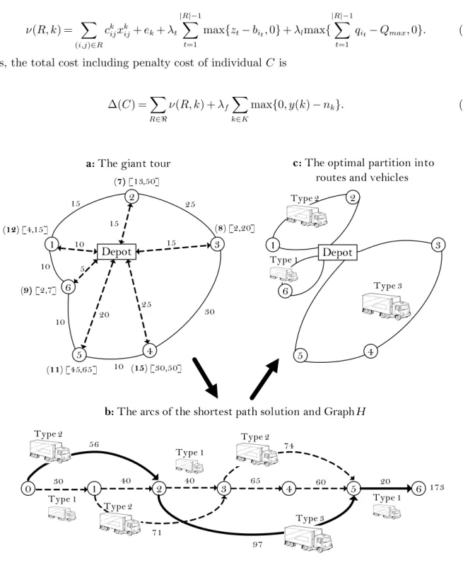
Figure 1 Illustration of procedureSplit
Figure 1 shows the steps of this advanced procedure using on an FD instance. The arc costs, demands and time windows are given in Figure 1a. In particular, the number in bold within the parentheses associated with each node is the demand for that customer; the two numbers within
brackets define the time window. Service times are identical and equal to 4 for each customer, and three different types of vehicles are available. The capacityqk and fixed costek of vehicles of type
{1,2,3} are q1= 10, q2= 20, q3= 30 and e1= 6, e2= 8, e3= 10, respectively. The algorithm starts with a giant TSP tour which includes six customers and uses one vehicle with unlimited capacity. The Splitalgorithm computes an optimal compound segmentation in three routes corresponding to three sequences of customers{1,2},{3,4,5}and{6}with three vehicle choices, Type 2, Type 3 and Type 1, respectively, as shown in Figure 1b. The resulting solution is shown in Figure 1c. An optimal partitioning of the giant tour into routes for offspring C corresponds to a minimum-cost path.
The penalty parameters of the Split algorithm are initially set to an initial value and are dynamically adjusted during the algorithm. If an individual is still infeasible after the first Educa-tionprocedure, then the penalty parameters are multiplied byλm and theEducationprocedure restarts. When this solution becomes feasible, the parameters are reset to their initial values.
2.6. Education
The Education procedure is systematically applied to each offspring in order to improve its quality. The ALNS algorithm is used as a way of educating the solutions in the HEA. This is achieved by applying both the destroy and repair operators, and a number of removable nodes are modified in each iteration. The operators used within the HEA are either adapted or inspired from those employed by various authors (Ropke and Pisinger 2006a,b, Pisinger and Ropke 2007, Demir et al. 2012, Paraskevopoulos et al. 2008). The Educationprocedure is detailed in Algorithm 2.
The removal procedure (Line 4 of Algorithm 2) runs for n′ iterations and removes n′ customers from the solution, wheren′ is in the interval of removable nodes [be
l, beu] for the first eight operators and is equal to the number of customers in the chosen route for the last operator.
The removal set of customers are added to the removal list Lr. An insertion operator is then selected to iteratively insert the nodes of Lrinto the partially destroyed solution untilLr is empty (Line 5). Feasibility conditions in terms of capacity and time windows are always respected during the insertion process. The removal and insertion operators are selected according to their past performance (see Section 2.5.3). The cost of an individual C before the removal is denoted by ω(C), and its cost after the insertion is denoted byω(C∗). An example of the removal and insertion phases is illustrated in Figure 2.
2.6.1. Removal Operators Nine removal operators are used in the destroy phase of the Educationprocedure and are described in detail below.
1.Random removal (RR): The RR operator randomly selects a node j∈N\{0}\Lr, removes it from the solution. The worst-case time complexity of the RR operator isO(n).
Algorithm 2Education 1: ω(C∗) = 0, iteration = 0
2: while there is no improvement andC is feasibledo
3: Lr=∅and select a removal operatord∈D
4: Apply a removal operatordto the individualC to remove a set of nodes and add them to Lr
5: Select an insertion operatorm∈M and apply it to the partially destroyed individualC to insert the nodes ofLr
6: LetC∗ be the new solution obtained by applying operator m 7: if iteration = 1 then
8: insert C∗ into the population 9: end if
10: if ω(C∗)< ω(C) andC∗ is feasiblethen 11: ω(C)←ω(C∗)
12: end if
13: iteration← iteration + 1 14: end while
15: Return educated feasible solution
Depot 8 2 10 3 4 11 5 7 1 9 6 Depot 8 2 10 3 4 11 5 7 1 9 6 Depot 8 2 10 3 4 11 5 7 1 9 6
a:A feasible solution b:A destroyed solution c:A repaired solution
Lr= Lr= {7,2,3} Lr=
Figure 2 Illustration of theEducationprocedure
2.Worst distance removal (WDR): The purpose of the WDR operator is to choose a number of expensive nodes according to their distance based cost. The cost of a node j∈N\{0}\Lr is the distance from its predecessor i and its distance to its successorj. The WDR operator iteratively
removes nodesj∗ from the solution wherej∗= arg max
j∈N\{0}\Lr{|dij+djk|}. The time complexity
of this operator is O(n2).
3.Worst time removal (WTR): The WTR operator is a variant of the WDR operator. For each node j∈N\{0}\Lr costs are calculated, depending on the deviation between the arrival time zj and the beginning of the time window aj. The WTR operator iteratively removes customers from the solution, wherej∗= arg max
j∈N\{0}\Lr{|zj−aj|}. The ALNS iteratively applies this process to
the solution after each removal. The WTR operator can be implemented in O(n2) time.
4.Neighborhood removal (NR): In a given solution with a set ℜ of routes, the NR operator calculates an average distance ¯d(R) =P(i,j)∈Rdij/|R| for each route R∈ ℜ, and selects a node j∗= arg max(
R∈ℜ;j∈R){d(R)¯ −dR\{j}}, wheredR\{j} denotes the distance of routeR excluding node j. The time complexity of this operator isO(n2).
5. Shaw removal (SR): The general idea behind the SR operator is to remove a set ofn′ similar customers. The similarity between two customers i and j is defined by the relatedness measure δ(i, j). This includes four terms: a distance termdij, a time term|ai−aj|, a relation termlij, which is equal to −1 ifiandj are in the same route, and 1 otherwise, and a demand term |qi−qj|. The relatedness measure is given by
δ(i, j) =ϕ1dij+ϕ2|ai−aj|+ϕ3lij+ϕ4|qi−qj|, (5) where ϕ1 toϕ4 are weights that are normalized to find the best candidate solution. The operator starts by randomly selecting a node i∈N\{0}\Lr, and selects the node j∗ to remove where j∗= arg minj∈N\{0}\Lr{δ(i, j)}. The operator is iteratively applied to select a node which is most similar
to the one last added toLr. The time complexity of this operator isO(n2).
6.Proximity-based removal(PBR): This operator is a second variant of the classical Shaw removal operator. The selection criterion of a set of routes is solely based on the distance. Therefore, the weights areϕ1= 1 andϕ2=ϕ3=ϕ4= 0. The PBR operator can be implemented in O(n2) time.
7. Time-based removal (TBR): The TBR operator removes a set of nodes that are related in terms of time. It is a special case of the Shaw removal operator whereϕ2= 1 andϕ1=ϕ3=ϕ4= 0. Its time complexity is O(n2).
8.Demand-based removal (DBR): The DBR operator is yet another variant of the Shaw removal operator with ϕ4= 1 and ϕ1=ϕ2=ϕ3= 0. It can be implemented in O(n2) time.
9. Average cost per unit removal (ACUTR): The average cost per unit (ACUT) is described by Paraskevopoulos et al. (2008) to measure the utilization efficiency of a vehicle Π(R) on a given routeR. Π(R) is expressed as the ratio of the total travel cost and fixed vehicle cost over the total demand carried by a vehiclek traversing routeR:
Π(R) = P (i,j)∈Acijxkij+ek P i∈N\{0}qixkij . (6)
The aim of the ACUTR operator is to calculate the cost of each route and remove the one with the least Π(R) value from the solution. The ACUTR operator can be implemented inO(n2) time.
2.6.2. Insertion Operators Three insertion operators are used in the repair phase of the Educationprocedure.
1. Greedy insertion (GI): The aim of this operator is to find the best possible insertion position for all nodes inLr. For node i∈N\Lr succeeded in the destroyed solution by k∈N\{0}\Lr, and node j∈Lr we define γ(i, j) =dij+djk−dik. We find the least-cost insertion position for j∈Lr by i∗= arg min
i∈N\Lr{γ(i, j)}. This process is iteratively applied to all nodes in Lr. The time
complexity of this operator isO(n2).
2.Greedy insertion with noise function(GINF): The GINF operator is based on the GI operator but extends it by allowing a degree of freedom in selecting the best place for a node. This is done by calculating the noise cost υ(i, j) =γ(i, j) +dmaxpnǫ wheredmax is the maximum distance between all nodes,pn is a noise parameter used for diversification and is set equal to 0.1, andǫis a random number in [−1,1]. The time complexity of this operator is O(n3).
3. Greedy insertion with en-route time (GIET): This operator calculates the en-route time dif-ferenceη(i, j) between before and after inserting the customerj∈Lr. For nodei∈N\Lr succeeded in the destroyed solution byk∈N\{0}\Lr, and nodej∈Lr, we defineη(i, j) =τij+τjk−τik where τij is the en-route time from node ito node j. We find the least-cost insertion position for j∈Lr by i∗= arg min
i∈N\Lr{η(i, j)}. The GIET operator can be implemented inO(n
2) time.
2.6.3. Adaptive Weight Adjustment Procedure Each removal and insertion operator has a certain probability of being chosen in every iteration. The selection criterion is based on the historical performance of every operator and is calibrated by a roulette-wheel mechanism (Ropke and Pisinger 2006a, Demir et al. 2012). Afteritw iterations of the roulette wheel segmentation, the probability of each operator is recalculated according to its total score. Initially, the probabilities of each removal and insertion operator are equal. Letpt
i be the probability of operatori in the last itwiterations,pti+1=pti(1−rp) +rpπi/τi, whererp is the roulette wheel probability, for operatori; πi is its score andτi is the number times it was used during the last segment. At the start of each segment, the scores of all operators are set to zero. The scores are changed by σ1 if a new best solution is found, byσ2 if the new solution is better than the current solution and byσ3if the new solution is worse than the current solution.
2.7. Intensification
We introduce a two-phase aggressive Intensification procedure to improve the quality of elite individuals. This procedure intensifies the search within promising regions of the solution space. The detailed pseude-code of this method is shown in Algorithm 3. The algorithm starts with an
elite list of solutionsLe, which takes the bestne individuals from the main population as measured by equation (2). Step 1 is similar to the mainEducationprocedure (Section 2.5). Step 2 attempts to explore different regions of the search space with the RR operator, intensifies this area by applying the GI operator for FD and HD, and GIET for FT and HT, to a partially the destroyed solution. Steps 1 and 2 terminate when there is no improvement to the solution and the main loop terminates whenne successive iterations have been performed.
2.8. Survivor Selection
In population-based metaheuristics, avoiding premature convergence is a key challenge. Ensuring the diversity of the population, in other words to search a different location in the solution space during the algorithm, in the hope of being closer to the best known or optimal solutions constitutes a major trade-off between solutions in a population. The method of Vidal et al. (2012), aims to ensure the diversity of the population and preserve the elite solutions. The second part of this method is the survivor selection process (the first part was discussed in Section 2.3). The algorithm starts with an initial population of size np, and after each iteration an offspring is added to the population. The maximum number of allowable offsprings in the population is shown byno. When the current population sizena reaches the maximum allowable size np+no, the survivor selection mechanism is put in place. This mechanism then selects np and discards no individuals from the population. The removal of no individuals is based on their biased fitness. In this way, elite individuals are protected.
2.9. Diversification
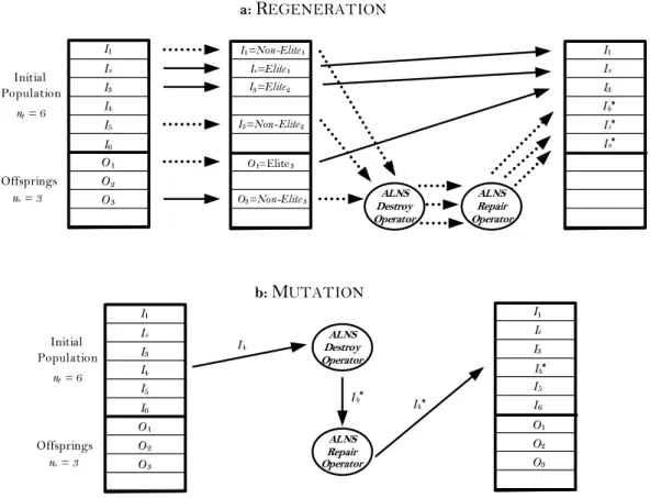
The efficient management of feasible solutions plays a significant role in population diversity. The performance of the HEA is improved by applying a Mutation after the Education procedure. Over the iterations, individuals tend to become more similar, making it difficult to avoid premature convergence. To overcome this difficulty, we introduce a new scheme in order to increase the population diversity. The diversification stage includes two procedures, namely Regeneration andMutation, representations of which are shown in Figure 3.
ARegenerationprocedure (Figure 3a) takes place when the maximum allowable iterations for Regenerationitris reached without an improvement in the best solution value. In this procedure, the ne elite individuals are preserved and are transferred to the next generation. The remaining np−neindividuals, which are ranked according to their biased fitness, are subjected to the RR and GINF operators, to create new individuals. At the end of this procedure, new individuals having various compositions are placed in the population.
The Mutation procedure is applied with probability pm. Figure 3b illustrates the Mutation procedure. In this procedure, an individualCdifferent from the best solution is randomly selected.
Algorithm 3Intensification 1: InitializeLe={O1, . . . , On},i←1
2: while all elite solutions are intensifieddo
3: O←Oi 4: Step 1
5: whilethere is no improvement and elite solutionO is feasibledo
6: Lr=∅and select a removal operatord∈D
7: Apply d∈D to the elite solutionO to remove nodes and add them toLr
8: Select an insertion operator m∈M and apply it to the destroyed elite solution O by inserting the node ofLr
9: Let O∗ be the new solution obtained by applying operatorm 10: if ω(O∗)< ω(O)then
11: ω(O)←ω(O∗)
12: end if
13: end while 14: Step 2
15: whilethere is no improvement andO is feasible do
16: Lr=∅ and apply RR operator to the elite solution O to remove nodes and add them toLr
17: Apply GI or GIET operator to the partially destroyed elite solutionO by inserting the node ofLr
18: Let O∗ be the new elite solution obtained by applying insertion operator 19: if ω(O∗)< ω(O)then
20: ω(O)←ω(O∗)
21: end if
22: end while
23: i←i+ 1 24: end while
25: Return elite solutions
Two randomized structure based ALNS operators, the RR and the GINF, are then used to change the positions of a specific number of nodes, which are chosen from the interval [bm
l , bmu] of removable nodes in the Mutationprocedure.
Initial Population I Offsprings I I I I I O O O n= 6 n= 3 I=Elite I =Elite O =Elite I =Non-Elite I =Non-Elite O =Non-Elite I I I Initial Population I Offsprings I I I I I O O O n= 6 n= 3 I I I I I a:REGENERATION b:MUTATION I I O O O I I I I I
Figure 3 Illustration of the diversification stage
3.
Computational Experiments
This section presents the results of computational experiments performed in order to assess the performance of the HEA. The HEA was implemented in C++ and run on a computer with one gigabyte RAM and Intel Xeon 2.6 GHz processor. We first describe the benchmark instances and the parameters used within the algorithm. This is followed by a presentation of the results.
3.1. Data Sets and Experimental Settings
The benchmark data sets of Liu and Shen (1999b), derived from the classical Solomon (1987) VRPTW instances with 100 nodes, are used as the test-bed. These sets include 56 instances, split into a random data set R, a clustered data set C and a semi-clustered data set RC. Sets shown by R1, C1 and RC1 have a short scheduling horizon and small vehicle capacities, in contrast to sets denoted R2, C2 and RC2 with a long scheduling horizon and large vehicle capacities. Liu and Shen (1999b) also introduced three cost structures, namely A, B and C, and several vehicle types with different capacities and fixed vehicle costs for each of the 56 instances. This results in a total of 168 benchmark instances for FT or FD.
The benchmark set used by Paraskevopoulos et al. (2008) for HT is a subset of the FT instances, in which the fleet size is set equal to that found in the best known solutions of Liu and Shen
(1999a). In total, there are 24 benchmark instances derived from Liu and Shen (1999a) for HT. We use the same set for HD, with the new objective.
Evolutionary algorithms use a set of correlated parameters and configuration decisions. In our implementation, we initially used the parameters suggested by Vidal et al. (2012, 2013) for the genetic algorithm, and by Demir et al. (2012) for the ALNS, but we have con-ducted several experiments to further fine-tune these parameters on instances C101A, C203A, R101A, R211A, RC105A and RC207A. Following these tests, the following parameter values were used in our experiments: itt= 5000, itr = 2000, itw = 500, np = 25, no = 25, ne = 10, nc = 3, pm∈[0.4,0.6],[bil, biu] = [0.3,0.8],[bel, beu] = [0.1,0.16],[bml , bmu] = [0.1,0.16], rp = 0.1, ϕ1= 0.5, ϕ2= 0.25, ϕ3= 0.15, ϕ4= 0.25, σ1= 3, σ2= 1, σ3= 0, λt=λl=λf= 3, λm= 10. These settings are identi-cal for all four considered problems.
Table 1 presents the results of a fine-tuning experiment on parameters np and no, and to test the effect of these parameters on the solution quality.
Table 1 Average percentage deviations of the solution values found by the HEA from best-known solution values with varyingnpandno
no np 10 25 50 75 100 10 0.42 0.26 0.38 0.56 0.69 25 0.19 0.11 0.26 0.37 0.49 50 0.39 0.29 0.30 0.45 0.57 75 0.56 0.42 0.51 0.61 0.68 100 0.67 0.53 0.61 0.72 0.78
The table shows the percent gap between the solution value obtained by the HEA and the best-known solution (BKS) value, averaged over the six chosen instances. The maximum population size is dependent on np and no, both of which have a significant impact on the solution quality, where the best setting is obtained with np=no= 25.
3.2. Comparative Analysis
We now present a comparative analysis of the results of the HEA with those reported in the literature. In particular, we compare ourselves against LSa (Liu and Shen 1999a), LSb (Liu and Shen 1999b), T-RR-TW (Dell’Amico et al. 2007), ReVNTS (Paraskevopoulos et al. 2008), MDA (Br¨aysy et al. 2008), BPDRT (Br¨aysy et al. 2009), AMP (Repoussis and Tarantilis 2010) and UHGS (Vidal et al. 2014). The comparisons are presented in Tables 2–4, where the columns show the total cost (TC), and percent deviations (Dev) of the values of solutions found by each method with respect to the HEA. The first column displays the instance sets and the number of instances in each set in parentheses. The rows named Avg (%), Min (%) and Max (%) show the average, minimum and maximum deviations across all benchmark instances, respectively. A negative deviation shows
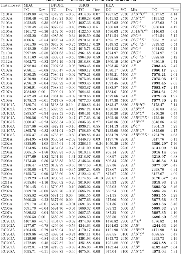
that the solution found by the HEA is of better quality. In the column labeled BKS, “=” shows the total number of matches and “<” shows the number of new BKS found for each instance set. Ten separate runs are performed for each instance, the best one of which is reported. For each instance, a boldface refers to match with current BKS, where as a boldface with a “*” indicates new BKS. For detailed results, the reader is referred to Appendix A. Tables A.1-A.6 present the fixed vehicle cost (VC), the distribution cost (DC), the computational time in minutes (Time) and the actual number of vehicles used (Mix) for the HEA.
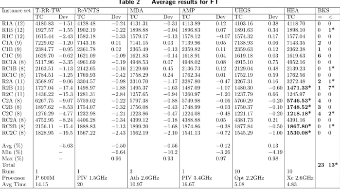
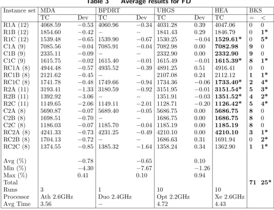
Tables 2 and 3 summarize the average comparison results of the current state-of-the-art solution methods for FT and FD, compared with the HEA. According to Tables 2 and 3, the HEA is highly competitive, with average deviations ranging from−5.63% to 0.13% and a worst-case performance of 0.98% for FT. As for FD, average cost reductions range from−0.78% to 0.10% and the worst case performance is 0.94%. The average performance of our HEA is better than that of all the competition, except for the algorithm of Vidal et al. (2014) which is slightly better on average. However, the HEA seems to outperforms this algorithm on to the second type of FT instances, which are less tight in terms of vehicle capacity.
Table 2 Average results for FT
Instance set T-RR-TW ReVNTS MDA AMP UHGS HEA BKS TC Dev TC Dev TC Dev TC Dev TC Dev TC = < R1A (12) 4180.83 −1.51 4128.48 −0.24 4131.31 −0.31 4113.89 0.12 4103.16 0.38 4118.70 0 0 R1B (12) 1927.57 −1.55 1902.19 −0.22 1898.88 −0.04 1896.83 0.07 1891.63 0.34 1898.10 0 1* R1C (12) 1615.44 −2.43 1582.18 −0.33 1579.17 −0.13 1578.12 −0.07 1574.32 0.17 1577.04 0 0 C1A (9) 7229.02 −1.20 7143.16 0.01 7141.15 0.03 7139.96 0.05 7138.93 0.06 7143.35 2 0 C1B (9) 2384.77 −0.95 2361.78 0.02 2365.49 −0.13 2359.82 0.11 2359.63 0.12 2362.38 1 0 C1C (9) 1629.70 −0.62 1621.09 −0.09 1621.83 −0.14 1618.91 0.04 1619.18 0.03 1619.63 6 0 RC1A (8) 5117.96 −3.35 4961.69 −0.19 4948.53 0.07 4948.02 0.08 4915.10 0.75 4952.16 0 0 RC1B (8) 2163.51 −1.13 2142.65 −0.16 2129.60 0.45 2136.73 0.12 2129.04 0.48 2139.23 0 1* RC1C (8) 1784.51 −1.25 1769.93 −0.42 1758.29 0.24 1762.34 0.01 1752.19 0.59 1762.56 0 0 R2A (11) 3568.97 −9.06 3304.57 −0.98 3310.70 −1.17 3287.80 −0.47 3267.31 0.16 3272.48 2 1* R2B (11) 1727.04 −17.4 1498.97 −1.88 1495.37 −1.63 1487.09 −1.07 1480.30 −0.60 1471.33* 1 7* R2C (11) 1436.22 −15.3 1281.31 −2.84 1257.65 −0.94 1260.97 −1.20 1237.79 0.66 1245.97 0 0 C2A (8) 6267.75 −9.07 5759.02 −0.22 5797.38 −0.88 5749.98 −0.06 5760.29 −0.20 5746.53* 4 0 C2B (8) 1897.62 −8.53 1754.07 −0.32 1756.08 −0.43 1748.99 −0.03 1750.37 −0.10 1748.52* 3 0 C2C (8) 1276.29 −4.77 1232.98 −1.21 1223.86 −0.47 1224.08 −0.48 1221.17 −0.20 1218.18* 4 2* RC2A (8) 4752.95 −8.24 4406.28 −0.34 4399.12 −0.18 4388.88 0.05 4381.73 0.21 4391.16 0 0 RC2B (8) 2156.11 −15.4 1888.83 −1.13 1899.20 −1.68 1874.86 −0.38 1877.84 −0.50 1867.80* 0 1* RC2C (8) 1828.95 −19.5 1567.22 −2.43 1562.19 −2.10 1541.13 −0.72 1545.29 −1.00 1530.08* 0 0 Avg (%) −5.63 −0.50 −0.56 −0.12 0.13 Min (%) − −6.64 −10.2 −3.26 −4.19 Max (%) − 0.96 0.93 0.97 0.98 Total 23 13* Runs 1 1 3 1 10 10
Processor P 600M PIV 1.5GHz Ath 2.6GHz PIV 3.4GHz Opt 2.2GHz Xe 2.6GHz Avg Time 14.15 20 10.97 16.67 5.08 4.83
Table 4 presents the comparison results for each HT instance against LSa and ReVNTS. We note that LSa originally solved FT, which was the basis for setting the number of available vehicles in ReVNTS. The results show that the HEA outperforms both methods and yields higher quality solutions within short computation times. On average, the total cost reductions obtained were
Table 3 Average results for FD
Instance set MDA BPDRT UHGS HEA BKS TC Dev TC Dev TC Dev TC = <
R1A (12) 4068.59 −0.53 4060.96 −0.34 4031.28 0.39 4047.06 0 0 R1B (12) 1854.60 −0.42 − − 1841.43 0.29 1846.79 0 1* R1C (12) 1539.48 −0.65 1539.90 −0.67 1530.25 −0.04 1529.61* 0 5* C1A (9) 7085.56 −0.04 7085.91 −0.04 7082.98 0.00 7082.98 9 0 C1B (9) 2335.11 −0.09 − − 2332.90 0.00 2332.90 9 0 C1C (9) 1615.75 −0.02 1615.40 −0.01 1615.49 −0.01 1615.39* 8 1* RC1A (8) 4944.48 −0.57 4935.52 −0.39 4891.25 0.51 4916.41 0 0 RC1B (8) 2121.62 −0.45 − − 2107.08 0.24 2112.12 1 1* RC1C (8) 1741.78 −0.48 1749.66 −0.94 1734.36 −0.06 1733.40* 2 4* R2A (11) 3193.41 −1.33 3180.59 −0.92 3151.95 −0.01 3151.54* 5 3* R2B (11) 1392.92 −3.06 − − 1351.91 −0.03 1351.52* 4 2* R2C (11) 1149.65 −2.06 1149.11 −2.01 1128.71 −0.20 1126.42* 5 4* C2A (8) 5690.87 −0.07 5689.40 −0.05 5686.75 0.00 5686.75 8 0 C2B (8) 1698.51 −0.70 − − 1686.75 0.00 1686.75 8 0 C2C (8) 1186.03 −0.07 1185.70 −0.04 1185.19 0.00 1185.19 8 0 RC2A (8) 4241.33 −0.73 4231.25 −0.49 4210.10 0.00 4210.10 3 1* RC2B (8) 1704.13 −0.72 − − 1686.63 0.31 1691.94 0 2* RC2C (8) 1374.55 −0.85 1385.32 −1.64 1358.24 0.34 1362.90 1 1* Avg (%) −0.78 −0.65 0.10 Min (%) −4.30 −7.67 −1.26 Max (%) 0.41 0.10 0.94 Total 71 25* Runs 3 1 10 10 Processor Ath 2.6GHz Duo 2.4GHz Opt 2.2GHz Xe 2.6GHz Avg Time 3.56 − 4.72 4.43
−12.68% and−0.34% compared to LSa and ReVNTS, with minimum deviations of−29.47% and
−2.01% and maximum deviations of −1.26% and 0.35%, respectively. Finally, Table 5 shows the results obtained on the newly introduced HD.
In summary, the HEA was able to find 36 BKS for 168 FT instances, where 14 are strictly better than those obtained by competing heuristics. As for FD, the algorithm has identified 96 BKS out of the 168 instances, 25 of which are strictly better. The results are even more striking for HT, with 17 BKS on the 24 instances, 14 of which are strictly better than those reported earlier. Overall, the HEA improves 52 BKS and matches 97 BKS out of 360 benchmark instances.
4.
Conclusions
We have proposed a unified heuristic for four types of heterogeneous fleet vehicle routing problems with time windows. The first two are the Fleet Size and Mix Vehicle Routing Problem with Time Windows (F) and the Heterogeneous Fixed Fleet Vehicle Routing Problem with Time Windows (H). Each of these two problems was solved under a time and a distance objective, yielding the four variants FT, FD, HT and HD. We have developed a unified hybrid evolutionary algorithm (HEA) capable of solving all variants without any modification. This heuristic combines state-of-the-art metaheuristic principles such as adaptive large scale neighborhood search and population search. We have integrated within our HEA an innovativeIntensificationstrategy on elite solutions and we have developed a new diversification scheme based on theRegenerationand theMutation
Table 4 Results for HT
Instance set LSa ReVNTS HEA BKS Mix TC Dev Mix TC Dev DC VC Mix TC Time = <
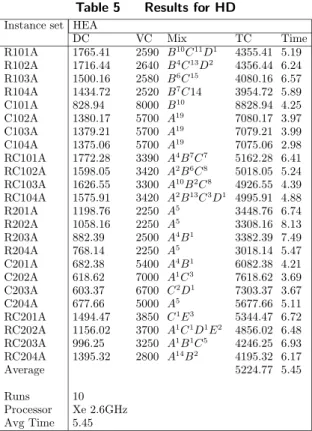
R101 A1B11C11D1 5061 −10.29 B10C11D1 4583.99 0.10 1998.76 2590 B10C11D1 4588.76 5.49 0 0 R102 A1B4C14D2 5013 −13.25 B3C14D2 4420.68 0.13 1736.54 2640 A1B4C13D2 4376.54* 6.78 0 1* R103 B7C15 4772 −13.57 B6C15 4195.05 0.16 1621.71 2580 B6C15 4201.71 7.45 0 0 R104 B9C14 4455 −10.61 B8C14 4065.52 −0.94 1487.69 2540 B9C13 4027.69* 6.14 0 1* C101 A1B10 9272 −5.02 B10 8828.93 0.00 828.93 8000 B10 8828.93 3.67 1 0 C102 A19 8433 −17.89 A19 7137.79 0.21 1453.13 5700 A19 7153.13 4.12 0 0 C103 A19 8033 −12.78 A19 7143.88 −0.30 1422.57 5700 A19 7122.57* 3.45 0 1* C104 A19 7384 −4.25 A19 7104.96 −0.30 1383.74 5700 A19 7083.74* 3.13 0 1* RC101 A7B7C7 5687 −7.99 A4B7C7 5279.92 −0.26 1876.36 3390 A4B7C7 5266.36* 5.73 0 1* RC102 A5B6C8 5649 −10.77 A4B5C8 5149.95 −0.99 1709.55 3390 A4B5C8 5099.55* 5.14 0 1* RC103 A11B2C8 5419 −8.58 A10B2C8 5002.41 −0.22 1691.29 3300 A10B2C8 4991.29* 4.90 0 1* RC104 A2B13C3D1 5189 −3.43 A2B13C3D1 5024.25 −0.15 1596.97 3420 A2B13C3D1 5016.97* 5.21 0 1* R201 A5 4593 −21.43 A5 3779.12 0.09 1532.49 2250 A5 3782.49 7.45 0 0 R202 A5 4331 −20.85 A5 3578.91 0.14 1333.92 2250 A5 3583.92 8.45 0 0 R203 A4B1 4220 −18.74 A4B1 3582.54 −0.81 1053.92 2500 A4B1 3553.92* 7.12 0 1* R204 A5 3849 −24.89 A5 3143.68 −2.01 831.80 2250 A5 3081.80* 6.99 0 1* C201 A4B1 6711 −9.29 A4B1 6140.64 0.00 740.64 5400 A4B1 6140.64 4.89 1 0 C202 A1C3 7720 −1.26 A1C3 7752.88 −1.69 623.96 7000 A1C3 7623.96* 4.26 0 1* C203 C2D1 7466 −2.23 C2D1 7303.37 0.00 603.37 6700 C2D1 7303.37 4.37 1 0 C204 A5 6744 −18.72 A5 5721.09 −0.72 680.46 5000 A5 5680.46* 5.29 0 1* RC201 C1E3 5871 −6.08 C1E3 5523.15 0.21 1684.59 3850 C1E3 5534.59 6.47 0 0 RC202 A1C1D1E2 5945 −15.43 A1C1D1E2 5132.08 0.35 1450.23 3700 A1C1D1E2 5150.23 6.35 0 0 RC203 A1B1C5 5790 −29.47 A1B1C5 4508.27 −0.81 1221.92 3250 A1B1C5 4471.92* 6.01 0 1* RC204 A14B2 4983 −17.47 A14B2 4252.87 −0.26 1441.83 2800 A14B2 4241.83* 5.87 0 1* Avg (%) −12.68 −0.34 Min (%) −29.47 −2.01 Max (%) −1.26 0.35 Total 3 14* Runs 3 1 10 Processor P 233M PIV 1.5GHz Xe 2.6GHz Avg Time − 20.00 5.61
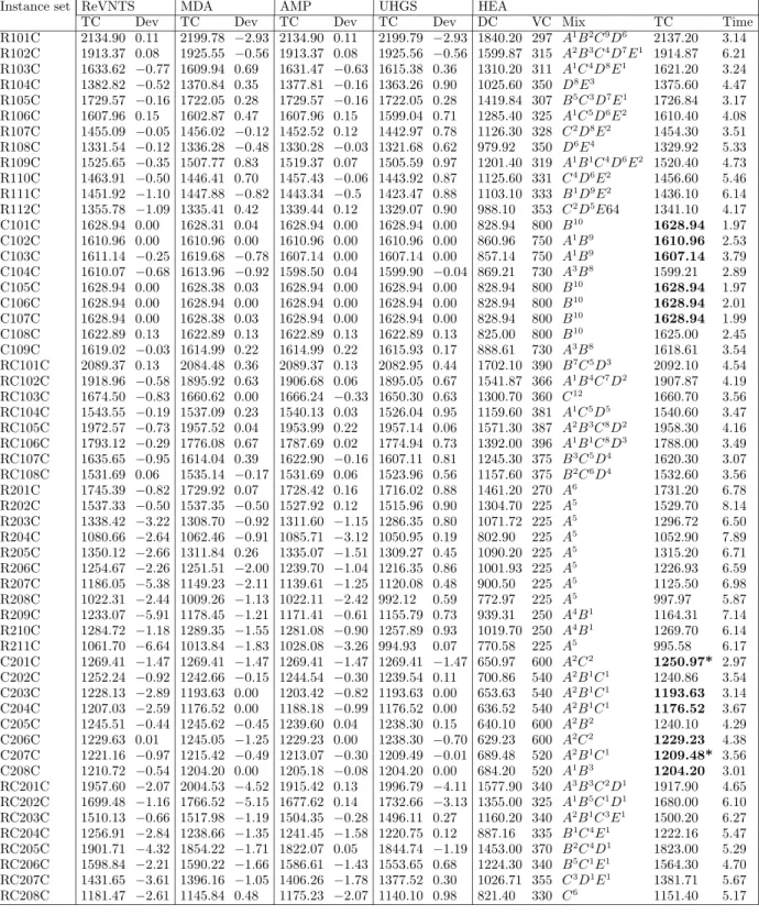
Table 5 Results for HD Instance set HEA
DC VC Mix TC Time R101A 1765.41 2590 B10C11D1 4355.41 5.19 R102A 1716.44 2640 B4C13D2 4356.44 6.24 R103A 1500.16 2580 B6C15 4080.16 6.57 R104A 1434.72 2520 B7C14 3954.72 5.89 C101A 828.94 8000 B10 8828.94 4.25 C102A 1380.17 5700 A19 7080.17 3.97 C103A 1379.21 5700 A19 7079.21 3.99 C104A 1375.06 5700 A19 7075.06 2.98 RC101A 1772.28 3390 A4B7C7 5162.28 6.41 RC102A 1598.05 3420 A2B6C8 5018.05 5.24 RC103A 1626.55 3300 A10B2C8 4926.55 4.39 RC104A 1575.91 3420 A2B13C3D1 4995.91 4.88 R201A 1198.76 2250 A5 3448.76 6.74 R202A 1058.16 2250 A5 3308.16 8.13 R203A 882.39 2500 A4B1 3382.39 7.49 R204A 768.14 2250 A5 3018.14 5.47 C201A 682.38 5400 A4B1 6082.38 4.21 C202A 618.62 7000 A1C3 7618.62 3.69 C203A 603.37 6700 C2D1 7303.37 3.67 C204A 677.66 5000 A5 5677.66 5.11 RC201A 1494.47 3850 C1E3 5344.47 6.72 RC202A 1156.02 3700 A1C1D1E2 4856.02 6.48 RC203A 996.25 3250 A1B1C5 4246.25 6.93 RC204A 1395.32 2800 A14B2 4195.32 6.17 Average 5224.77 5.45 Runs 10 Processor Xe 2.6GHz Avg Time 5.45
of solutions. We have also developed an advanced version of the Split algorithm of Prins (2009) to determine the best fleet mix for a set of routes. Finally, we have introduced the new variant HD. Extensive computational experiments were carried out on benchmark instances. In the case of FT and FD, our HEA clearly outperforms all previous algorithms except that of Vidal et al. (2014). In the latter case, it performs slightly worse on average, but seems to be superior on instances which are less tight in terms of vehicle capacity. Overall, the HEA has identified 132 new best solutions out of 336 on the F instances, 39 of which are strictly better. On the HT instances, our HEA outperforms the two existing algorithms and has identified 17 best known solutions out of 24, 14 of which are strictly better. The HD instances are solved here for the first time. Overall, we have improved 52 solutions out of 360 instances, and we have matched 97 others. All instances were solved within a modest computational effort. Our algorithm is not only highly competitive, but it is also flexible in that it can solve four problem classes with the same parameter settings.
Acknowledgments
The authors gratefully acknowledge funding provided by the Southampton Management School at the Uni-versity of Southampton and by the Canadian Natural Sciences and Engineering Research Council under grants 39682-10 and 436014-2013.
Appendix
Table A.1 Results for FT for cost structure A
Instance set ReVNTS MDA AMP UHGS HEA
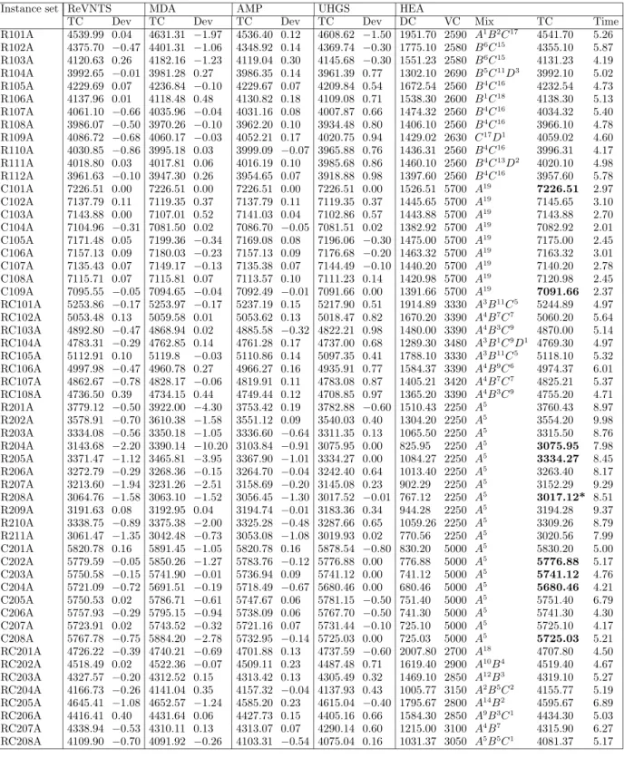
TC Dev TC Dev TC Dev TC Dev DC VC Mix TC Time R101A 4539.99 0.04 4631.31 −1.97 4536.40 0.12 4608.62 −1.50 1951.70 2590 A1B2C17 4541.70 5.26 R102A 4375.70 −0.47 4401.31 −1.06 4348.92 0.14 4369.74 −0.30 1775.10 2580 B6C15 4355.10 5.87 R103A 4120.63 0.26 4182.16 −1.23 4119.04 0.30 4145.68 −0.30 1551.23 2580 B6C15 4131.23 4.19 R104A 3992.65 −0.01 3981.28 0.27 3986.35 0.14 3961.39 0.77 1302.10 2690 B5C11D3 3992.10 5.02 R105A 4229.69 0.07 4236.84 −0.10 4229.67 0.07 4209.84 0.54 1672.54 2560 B4C16 4232.54 4.73 R106A 4137.96 0.01 4118.48 0.48 4130.82 0.18 4109.08 0.71 1538.30 2600 B1C18 4138.30 5.13 R107A 4061.10 −0.66 4035.96 −0.04 4031.16 0.08 4007.87 0.66 1474.32 2560 B4C16 4034.32 5.40 R108A 3986.07 −0.50 3970.26 −0.10 3962.20 0.10 3934.48 0.80 1406.10 2560 B4C16 3966.10 4.78 R109A 4086.72 −0.68 4060.17 −0.03 4052.21 0.17 4020.75 0.94 1429.02 2630 C17D1 4059.02 4.60 R110A 4030.85 −0.86 3995.18 0.03 3999.09 −0.07 3965.88 0.76 1436.31 2560 B4C16 3996.31 4.17 R111A 4018.80 0.03 4017.81 0.06 4016.19 0.10 3985.68 0.86 1460.10 2560 B4C13D2 4020.10 4.98 R112A 3961.63 −0.10 3947.30 0.26 3954.65 0.07 3918.88 0.98 1397.60 2560 B4C16 3957.60 5.78 C101A 7226.51 0.00 7226.51 0.00 7226.51 0.00 7226.51 0.00 1526.51 5700 A19 7226.51 2.97 C102A 7137.79 0.11 7119.35 0.37 7137.79 0.11 7119.35 0.37 1445.65 5700 A19 7145.65 3.10 C103A 7143.88 0.00 7107.01 0.52 7141.03 0.04 7102.86 0.57 1443.88 5700 A19 7143.88 2.70 C104A 7104.96 −0.31 7081.50 0.02 7086.70 −0.05 7081.51 0.02 1382.92 5700 A19 7082.92 2.01 C105A 7171.48 0.05 7199.36 −0.34 7169.08 0.08 7196.06 −0.30 1475.00 5700 A19 7175.00 2.45 C106A 7157.13 0.09 7180.03 −0.23 7157.13 0.09 7176.68 −0.20 1463.32 5700 A19 7163.32 3.01 C107A 7135.43 0.07 7149.17 −0.13 7135.38 0.07 7144.49 −0.10 1440.20 5700 A19 7140.20 2.78 C108A 7115.71 0.07 7115.81 0.07 7113.57 0.10 7111.23 0.14 1420.98 5700 A19 7120.98 2.45 C109A 7095.55 −0.05 7094.65 −0.04 7092.49 −0.01 7091.66 0.00 1391.66 5700 A19 7091.66 2.37 RC101A 5253.86 −0.17 5253.97 −0.17 5237.19 0.15 5217.90 0.51 1914.89 3330 A3B11C5 5244.89 4.97 RC102A 5053.48 0.13 5059.58 0.01 5053.62 0.13 5018.47 0.82 1670.20 3390 A4B7C7 5060.20 5.64 RC103A 4892.80 −0.47 4868.94 0.02 4885.58 −0.32 4822.21 0.98 1480.00 3390 A4B3C9 4870.00 5.14 RC104A 4783.31 −0.29 4762.85 0.14 4761.28 0.17 4737.00 0.68 1289.30 3480 A3B1C9D1 4769.30 4.97 RC105A 5112.91 0.10 5119.8 −0.03 5110.86 0.14 5097.35 0.41 1788.10 3330 A3B11C5 5118.10 5.32 RC106A 4997.98 −0.47 4960.78 0.27 4966.27 0.16 4935.91 0.77 1584.37 3390 A4B9C6 4974.37 6.01 RC107A 4862.67 −0.78 4828.17 −0.06 4819.91 0.11 4783.08 0.87 1405.21 3420 A4B7C7 4825.21 5.37 RC108A 4736.50 0.39 4734.15 0.44 4749.44 0.12 4708.85 0.97 1365.20 3390 A4B3C9 4755.20 4.71 R201A 3779.12 −0.50 3922.00 −4.30 3753.42 0.19 3782.88 −0.60 1510.43 2250 A5 3760.43 8.97 R202A 3578.91 −0.70 3610.38 −1.58 3551.12 0.09 3540.03 0.40 1304.20 2250 A5 3554.20 9.98 R203A 3334.08 −0.56 3350.18 −1.05 3336.60 −0.64 3311.35 0.13 1065.50 2250 A5 3315.50 8.76 R204A 3143.68 −2.20 3390.14 −10.20 3103.84 −0.91 3075.95 0.00 825.95 2250 A5 3075.95 7.98 R205A 3371.47 −1.12 3465.81 −3.95 3367.90 −1.01 3334.27 0.00 1084.27 2250 A5 3334.27 8.45 R206A 3272.79 −0.29 3268.36 −0.15 3264.70 −0.04 3242.40 0.64 1013.40 2250 A5 3263.40 8.17 R207A 3213.60 −1.94 3231.26 −2.51 3158.69 −0.20 3145.08 0.23 902.29 2250 A5 3152.29 9.29 R208A 3064.76 −1.58 3063.10 −1.52 3056.45 −1.30 3017.52 −0.01 767.12 2250 A5 3017.12* 8.51 R209A 3191.63 0.08 3192.95 0.04 3194.74 −0.01 3183.36 0.34 944.28 2250 A5 3194.28 9.37 R210A 3338.75 −0.89 3375.38 −2.00 3325.28 −0.48 3287.66 0.65 1059.26 2250 A5 3309.26 8.79 R211A 3061.47 −1.35 3042.48 −0.73 3053.08 −1.08 3019.93 0.02 770.56 2250 A5 3020.56 7.99 C201A 5820.78 0.16 5891.45 −1.05 5820.78 0.16 5878.54 −0.80 830.20 5000 A5 5830.20 5.00 C202A 5779.59 −0.05 5850.26 −1.27 5783.76 −0.12 5776.88 0.00 776.88 5000 A5 5776.88 5.17 C203A 5750.58 −0.15 5741.90 −0.01 5736.94 0.09 5741.12 0.00 741.12 5000 A5 5741.12 4.76 C204A 5721.09 −0.72 5691.51 −0.19 5718.49 −0.67 5680.46 0.00 680.46 5000 A5 5680.46 4.21 C205A 5750.53 0.02 5786.71 −0.61 5747.67 0.06 5781.15 −0.50 751.40 5000 A5 5751.40 6.79 C206A 5757.93 −0.29 5795.15 −0.94 5738.09 0.06 5767.70 −0.50 741.30 5000 A5 5741.30 4.30 C207A 5723.91 0.02 5743.52 −0.32 5721.16 0.07 5731.44 −0.10 725.10 5000 A5 5725.10 4.17 C208A 5767.78 −0.75 5884.20 −2.78 5732.95 −0.14 5725.03 0.00 725.03 5000 A5 5725.03 5.21 RC201A 4726.22 −0.39 4740.21 −0.69 4701.88 0.13 4737.59 −0.60 2007.80 2700 A18 4707.80 4.50 RC202A 4518.49 0.02 4522.36 −0.07 4509.11 0.23 4487.48 0.71 1619.40 2900 A10B4 4519.40 4.67 RC203A 4327.57 −0.20 4312.52 0.15 4313.42 0.13 4305.49 0.32 1469.10 2850 A12B3 4319.10 5.27 RC204A 4166.73 −0.26 4141.04 0.35 4157.32 −0.04 4137.93 0.43 1005.77 3150 A2B5C2 4155.77 5.19 RC205A 4645.41 −1.08 4652.57 −1.24 4585.20 0.23 4615.04 −0.40 1795.67 2800 A14B2 4595.67 6.89 RC206A 4416.41 0.40 4431.64 0.06 4427.73 0.15 4405.16 0.66 1584.30 2850 A9B3C1 4434.30 5.03 RC207A 4338.94 −0.53 4310.11 0.13 4313.07 0.07 4290.14 0.60 1215.00 3100 A4B7 4315.90 6.27 RC208A 4109.90 −0.70 4091.92 −0.26 4103.31 −0.54 4075.04 0.16 1031.37 3050 A5B5C1 4081.37 5.17
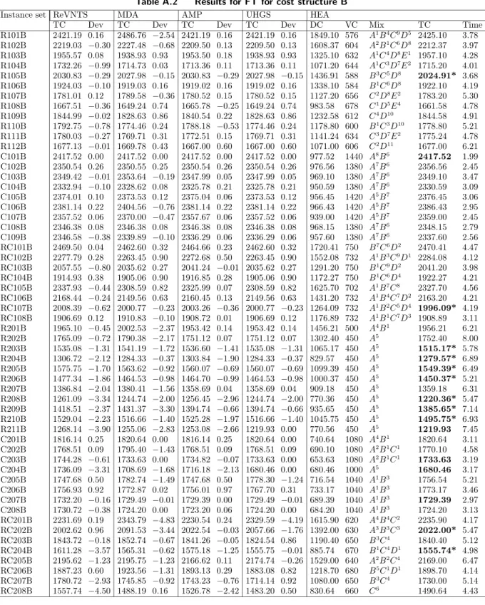
Table A.2 Results for FT for cost structure B
Instance set ReVNTS MDA AMP UHGS HEA
TC Dev TC Dev TC Dev TC Dev DC VC Mix TC Time R101B 2421.19 0.16 2486.76 −2.54 2421.19 0.16 2421.19 0.16 1849.10 576 A1B4C9D5 2425.10 3.78 R102B 2219.03 −0.30 2227.48 −0.68 2209.50 0.13 2209.50 0.13 1608.37 604 A2B1C6D8 2212.37 3.97 R103B 1955.57 0.08 1938.93 0.93 1953.50 0.18 1938.93 0.93 1325.10 632 A1C4D8E1 1957.10 4.28 R104B 1732.26 −0.99 1714.73 0.03 1713.36 0.11 1713.36 0.11 1071.20 644 A1C3D7E2 1715.20 4.01 R105B 2030.83 −0.29 2027.98 −0.15 2030.83 −0.29 2027.98 −0.15 1436.91 588 B3C5D8 2024.91* 3.68 R106B 1924.03 −0.10 1919.03 0.16 1919.02 0.16 1919.02 0.16 1338.10 584 B1C6D8 1922.10 4.19 R107B 1781.01 0.12 1789.58 −0.36 1780.52 0.15 1780.52 0.15 1127.20 656 C2D8E2 1783.20 5.30 R108B 1667.51 −0.36 1649.24 0.74 1665.78 −0.25 1649.24 0.74 983.58 678 C1D5E4 1661.58 4.78 R109B 1844.99 −0.02 1828.63 0.86 1840.54 0.22 1828.63 0.86 1232.58 612 C4D10 1844.58 4.91 R110B 1792.75 −0.78 1774.46 0.24 1788.18 −0.53 1774.46 0.24 1178.80 600 B1C3D10 1778.80 5.21 R111B 1780.03 −0.27 1769.71 0.31 1772.51 0.15 1769.71 0.31 1141.24 634 C3D7E2 1775.24 4.78 R112B 1677.13 −0.01 1669.78 0.43 1667.00 0.60 1667.00 0.60 1071.00 606 C2D11 1677.00 6.21 C101B 2417.52 0.00 2417.52 0.00 2417.52 0.00 2417.52 0.00 977.52 1440 A8B6 2417.52 1.99 C102B 2350.54 0.26 2350.55 0.25 2350.54 0.26 2350.54 0.26 976.56 1380 A7B6 2356.56 2.45 C103B 2349.42 −0.01 2353.64 −0.19 2347.99 0.05 2347.99 0.05 969.10 1380 A7B6 2349.10 3.47 C104B 2332.94 −0.10 2328.62 0.08 2325.78 0.21 2325.78 0.21 950.59 1380 A7B6 2330.59 3.09 C105B 2374.01 0.10 2373.53 0.12 2375.04 0.06 2373.53 0.12 956.45 1420 A5B7 2376.45 3.06 C106B 2381.14 0.22 2404.56 −0.76 2381.14 0.22 2381.14 0.22 966.43 1420 A5B7 2386.43 2.95 C107B 2357.52 0.06 2370.00 −0.47 2357.67 0.06 2357.52 0.06 939.00 1420 A5B7 2359.00 2.45 C108B 2346.38 0.08 2346.38 0.08 2346.38 0.08 2346.38 0.08 968.15 1380 A7B6 2348.15 2.79 C109B 2346.58 −0.38 2339.89 −0.10 2336.29 0.06 2336.29 0.06 957.60 1380 A7B6 2337.60 2.56 RC101B 2469.50 0.04 2462.60 0.32 2464.66 0.23 2462.60 0.32 1720.41 750 B7C6D2 2470.41 4.47 RC102B 2277.79 0.28 2263.45 0.90 2272.68 0.50 2263.45 0.90 1552.08 732 A1B3C9D1 2284.08 4.12 RC103B 2057.55 −0.80 2035.62 0.27 2041.24 −0.01 2035.62 0.27 1291.20 750 B1C9D2 2041.20 3.98 RC104B 1914.93 0.38 1905.06 0.90 1916.85 0.28 1905.06 0.90 1172.27 750 B1C6D4 1922.27 4.21 RC105B 2337.93 −0.44 2308.59 0.82 2325.99 0.07 2308.59 0.82 1625.70 702 A1B7C8 2327.70 4.56 RC106B 2168.44 −0.24 2149.56 0.63 2160.45 0.13 2149.56 0.63 1431.20 732 A1B4C7D2 2163.20 4.21 RC107B 2008.39 −0.62 2000.77 −0.23 2003.26 −0.36 2000.77 −0.23 1264.09 732 A1B2C5D4 1996.09* 4.19 RC108B 1906.69 0.12 1910.83 −0.10 1908.72 0.01 1906.69 0.12 1176.89 732 A1B1C7D3 1908.89 3.11 R201B 1965.10 −0.45 2002.53 −2.37 1953.42 0.14 1953.42 0.14 1456.21 500 A4B1 1956.21 6.21 R202B 1765.09 −0.72 1790.38 −2.17 1751.12 0.07 1751.12 0.07 1302.40 450 A5 1752.40 8.00 R203B 1535.08 −1.31 1541.19 −1.72 1536.60 −1.41 1535.08 −1.31 1065.17 450 A5 1515.17* 5.78 R204B 1306.72 −2.12 1284.33 −0.37 1303.84 −1.90 1284.33 −0.37 829.57 450 A5 1279.57* 6.89 R205B 1575.75 −1.70 1563.62 −0.92 1560.07 −0.69 1560.07 −0.69 1099.39 450 A5 1549.39* 6.49 R206B 1477.34 −1.86 1464.53 −0.98 1464.70 −0.99 1464.53 −0.98 1000.37 450 A5 1450.37* 5.21 R207B 1386.84 −2.04 1380.41 −1.56 1358.69 0.04 1358.69 0.04 909.18 450 A5 1359.18 6.31 R208B 1261.09 −3.34 1244.74 −2.00 1256.45 −2.96 1244.74 −2.00 770.36 450 A5 1220.36* 5.47 R209B 1418.51 −2.37 1431.37 −3.30 1394.74 −0.66 1394.74 −0.66 935.65 450 A5 1385.65* 7.14 R210B 1529.04 −2.23 1516.66 −1.40 1525.28 −1.97 1516.66 −1.40 1045.75 450 A5 1495.75* 6.93 R211B 1268.14 −3.90 1255.06 −2.83 1253.08 −2.66 1219.93 0.00 770.56 450 A5 1219.93 7.45 C201B 1816.14 0.25 1820.64 0.00 1816.14 0.25 1820.64 0.00 740.64 1080 A4B1 1820.64 3.11 C202B 1768.51 0.09 1795.40 −1.43 1768.51 0.09 1768.51 0.09 690.10 1080 A2B1C1 1770.10 4.58 C203B 1744.28 −0.61 1733.63 0.00 1734.82 −0.07 1733.63 0.00 653.63 1080 A2B1C1 1733.63 3.19 C204B 1736.09 −3.31 1708.69 −1.68 1716.18 −2.13 1680.46 0.00 680.46 1000 A5 1680.46 3.17 C205B 1747.68 0.50 1782.74 −1.49 1747.68 0.50 1778.30 −1.24 716.54 1040 A1B3 1756.54 5.21 C206B 1756.93 0.92 1772.87 0.02 1756.01 0.97 1767.70 0.31 733.17 1040 A1B3 1773.17 3.46 C207B 1732.20 −0.16 1729.49 −0.01 1729.39 0.00 1729.49 −0.01 689.39 1040 A1B3 1729.39 2.97 C208B 1730.72 −0.38 1724.20 0.00 1723.20 0.06 1724.20 0.00 684.20 1040 A1B3 1724.20 3.13 RC201B 2231.69 0.19 2343.79 −4.83 2230.54 0.24 2329.59 −4.19 1615.90 620 A4B4C2 2235.90 4.17 RC202B 2002.62 0.96 2091.53 −3.44 2022.54 −0.03 2057.66 −1.76 1392.00 630 A3B3C3 2022.00* 5.47 RC203B 1843.72 −0.18 1852.74 −0.67 1841.26 −0.05 1824.54 0.86 1190.40 650 B3C4 1840.40 5.12 RC204B 1611.28 −3.57 1565.31 −0.62 1575.18 −1.25 1555.75 −0.01 885.74 670 B1C4D1 1555.74* 4.98 RC205B 2195.62 −1.23 2195.75 −1.23 2166.62 0.11 2174.74 −0.26 1529.00 640 A2B2C4 2169.00 6.47 RC206B 1887.23 0.60 1923.56 −1.31 1893.13 0.29 1883.08 0.82 1218.70 680 B5C1D1 1898.70 4.14 RC207B 1780.72 −2.93 1745.85 −0.92 1743.23 −0.76 1714.14 0.92 1080.00 650 B3C4 1730.00 5.14 RC208B 1557.74 −4.50 1488.19 0.16 1526.78 −2.42 1483.20 0.50 830.64 660 C6 1490.64 4.43