Fuzzy logic in computer game strategies Fine-tuning artificial intelligence strategy selection

Fuzzy logic

in computer game strategies

Vincent Lichtenberg

ANR: 868438

HAIT Master Thesis series nr. 13-001

Thesis submitted in partial fulfillment of the requirements for the degree of

Master of Arts in Communication and Information Sciences, Master Track Human Aspects of Information Technology,

at the School of humanities of Tilburg University

Thesis committee: dr. ir. P.H.M. Spronck2

Prof. dr. H.J. van den Herik3

Prof. dr. A. Plaat

Tilburg University School of Humanities

Department of Communication and Information Sciences Tilburg center for Cognition and Communication (TiCC)

Tilburg, The Netherlands

May 29, 2013 1 [email protected] 2_{[email protected]} 3 [email protected]

Contents

2.1.1 AI in Real Time Strategy games . . . 4

2.1.2 Adaptive AI . . . 4 2.1.3 Case bases . . . 5 2.2 Fuzzy logic . . . 6 2.3 Data mining . . . 7 2.4 Casanova . . . 9 3 Experimental setup 10 3.1 The game . . . 10 3.1.1 Goal . . . 10 3.1.2 Specifics . . . 10 3.1.3 Implementation . . . 11 3.2 Simulations . . . 11 3.2.1 Strategy configurations . . . 12 3.2.2 Limitations . . . 14

3.3 Experiment I: Fuzzy logic classification . . . 14

3.4 Experiment II: Data mining . . . 18

4 Results 20 4.1 Fuzzy logic experiments . . . 20

4.2 Data Mining experiment . . . 23

4.3 Predictions . . . 25 4.3.1 Plots . . . 27 4.3.2 Statistics . . . 30 5 Discussion 31 5.1 Discussing results . . . 31 5.2 Limitations . . . 32 5.2.1 Case base . . . 32 5.2.2 The game . . . 32 5.3 Future work . . . 33

6 Conclusions 35 References 37 Appendices 39 A Statistics 39 A.1 Settings . . . 39 A.1.1 IBk . . . 39 A.1.2 J48 . . . 40 A.1.3 MultiLayerPerceptron . . . 40

Abstract

Although audiovisual qualities of computer games have been improving vastly over the years, the artificial intelligence of virtual adversaries still offers room for improvement. One of the aspects that can be improved is adaptation: while human players adapt to certain events, AI-controlled players sturdily follow pre-defined flowcharts with instructions that do not respond to dynamic cir-cumstances. The goal of this investigation is to enable an AI to generate an appropriate counter response against a specific enemy AI.

This investigation proposes a way of implementing adaptive AI strategies based on fuzzy logic theory. A case base was generated which was then analysed by three different fuzzy logic-based algorithms in order to find the strongest possible counter strategy settings, based on a provided enemy strategy. Also, four data mining classifiers were trained on the case base to investigate the possibility of classifying the outcome of a match given certain settings.

The results of an experiment wherein 10 randomly picked enemies were coun-tered by strategies recommended by the fuzzy logic algorithms were convincing: 66.51% of all matches were won by the fuzzy classifiers, where counters from the Min lose algorithm scored highest by winning 70.33% of all matches. These winning percentages of these counters were considerably higher than the base-line winning chances, from which can be concluded that fuzzy logic theory is indeed suitable for the improvement of game AI strategy selection.

Preface

As long as I remember, I have been playing computer games. It all began with the Atari ST and playing games from 3,5” floppy disks on my father’s PC. When I got my very own Pentium 166 MHz PC and PlayStation (the first one, indeed), this passion could no longer be stopped.

In retrospective, I’m glad that nobody tried, for it eventually became an important part of my education. After all, not many people get to say that they graduated on something as fun as computer games.

When my Master-course had started for a few weeks, I thought it would be sensible to start orienting on possible graduation subjects. I ultimately ended up with fuzzy logic because of a lecture by Pieter Spronck, my thesis supervisor, in which he covered the subject during the Computer Games course. After some deliberation, it struck us as a good idea to apply the ideology behind fuzzy logic in choosing strategies in computer games.

After a few months, it has all come down to the thesis that lies in front of you. This thesis describes my intensive and educational graduation project, and I hope you will enjoy and perhaps even get inspired reading it.

Acknowledgements

This thesis would not have been possible without the guidance of Pieter Spronck. I would like to thank him for inspirational suggestions for the experiments, whilst keeping everything on track, and for all the laughs I had because of his rants about how bad the AI in modern games often is. I hereby also would like to thank Jaap van den Herik for his advice on writing this thesis.

I would also like to thank Giuseppe Maggiore for the council and effort he has put into makingCasanovaavailable as a simulation platform. A special thanks goes out to Mohamed Adibi, who focused on making Casanova operable for this thesis project.

Also, I would like to thank Aske Plaat for his interest in this project, and for eventually being part of the thesis committee.

I would like to thank all of my friends for all of their mental support. Blowing off steam and having people listening to endless speeches about my research are essential to a successful track. A special thanks goes out to Chris Emmery, for always providing a good atmosphere for our rightfully claimed office: the HAIT lab. A positive mindset is an important ingredient to a successful graduation, so it is gratefully appreciated.

Of course, I would like to thank my parents and brother for their support as well. My mother Karin and my father Jos (being a professor in architecture and engineering) have always made it possible and stimulated me into carrying on studying. Everything I’ve learned from my studies, I have you to thank for. My brother Sebastiaan is finishing his master’s graduation as well, and I wish him all the best with the proverbial last miles of his graduation course.

Last but not least I would like to thank my lovely girlfriend Lieke, for putting up with me the last few months. The last 2-3 months must’ve been tough, but you’re finally getting your boyfriend back now, both physically and mentally. Thank you for understanding!

Chapter 1

Introduction

Ever since computers have been considered gaming platforms, various aspects of computer games have been evolving rapidly over the years. Two of the very first computer games, Pong (1972) and Tetris (1984), had minimal graphics. Along with computational capacity, audiovisual qualities have been developing exponentially over time. One particular computer game element, however, de-veloped at a relatively low ebb: artificial intelligence (hereafter abbreviated as ‘AI’) [6].

A highly plausible reason for focussing on development of audiovisual ele-ments of a computer game (hereafter referred to as ‘game’), is that it is impor-tant for game developers - and especially distributors - to be able to actually show the qualities of their products to the world. One can imagine that flaunting impressive artwork and in-game footage from their latest games in advertising campaigns is more effective than giving a description of how realistic the be-haviour of game world elements is.

Nevertheless, the fact remains that games with relatively simple graphics can still be successful [10]. The popularity of games such as Riot’s League of Legends1 _{and Blizzard’s World of Warcraft}2 _{and StarCraft II}3 _{underlines this.}

What these three games also have in common is that they allow players all over the world to play with and against each other, rendering the experience of playing these games more diverse and challenging.

The game AI in triple-A games such as League of Legends and StarCraft II, however, remains inferior and offers room for improvement[6, 1, 13, 17]. There are different aspects of game AI that can be enhanced, such as skill, effectiveness, adaptability, or showing more human-like behaviour. Although certain elements in a game seem to react on the player’s actions, unrealistic scenarios still occur. For instance, a computer-controlled soldier may not respond to the fact that one of his colleagues has just been shot dead right next to him. If this soldier were to be controlled by a human player, it would be adapting to this threatening situation and thus be thinking about the best possible strategy to overcome it. For games to remain challenging, and with that interesting, game AI oppo-nents should be adapting (i.e., acting more dynamically) to what is happening in the virtual world: an action of the human player should lead to an appro-priate reaction from the game AI. The game AI should therefore be capable of interpreting the perceived strategy of its adversary, and executing anticipating strategies based on this interpretation.

This thesis research investigates the possibility of implementing anticipation into a game AI, enabling it to formulate a suitable counter strategy based on its

1_{League of Legends official website: http://euw.leagueoflegends.com/} 2_{World of warcraft official website: http://eu.battle.net/wow/en/} 3_{StarCraft II official Battle.net website: http://eu.battle.net/sc2/en/}

situation. Given the strategy of its adversary, the game AI should be capable of formulating an adequate counter strategy. With that, it is vital to understand how such a game AI can reason about choosing strategies that are suitable in certain conditions.

1.1

Problem statement

This thesis research investigates if the selection of adaptive game AI strategies can be refined. Therefore, the following problem statement is posed: To what extent is it possible to improve strategy selection by a computer game AI by the application of fuzzy logic theory? This leads to the following research questions:

(i) What research has been done on adaptive game AI?

It is important to know what other researchers have done to implement adaptability into a game AI. This leads to the next research question:

(ii) How does an adaptive game AI determine a suitable strategy for a specific situation?

What methods are used to ‘teach’ a game AI on what strategies are effective in certain circumstances? Such a counter strategy should, of course, be more refined than just an ‘all-out attack’ command, which gives the third research question:

(iii) How can nuances be induced into a strategy?

The effectiveness of this selected nuanced strategy needs to be tested, which leads to the fourth research question:

(iv) How effective are the selected counter strategies?

1.2

Methodology

In order to answer the four research questions, the following steps have to be taken. The first step is to explore earlier research on adaptive game AI. The focus on this search will be strategy games; specifically Real Time Strategy (RTS) games. An RTS game is where multiple players build and move their units strategically within an environment, ultimately destroying the units of their opponents. RTS games are suitable for this type of research, as tactics are relatively easy to model (e.g., army sizes and movement directions are measur-able).

Exploration of earlier adaptive game AI research will automatically lead to methods of artificial strategy determination as well. Since the focus of this research is to determine a suitable counter strategy for certain situations, the opposing strategy that is to be countered, is provided.

Determining a suitable counter reaction to the enemy strategy is, in most cases, a subtle task, for it is desirable that a game AI can balance its focus on various aspects in a strategy. A human player would, in most cases, not only focus on building an army, as this renders his4 _{defence vulnerable should the}

attack fail. This research will investigate to what extent fuzzy logic theory (as explained in Section 2.2) can enable a game AI to make strategic decisions.

Once this ‘fuzzy logic strategy algorithm’ is created, the effectiveness of the counters it provides needs to be measured. This will be measured by running simulations in a platform calledCasanova (further explained in Section 2.4). Various sophisticated data mining techniques (Section 2.3) are applied on the dataset as well. The fuzzy logic strategy algorithm is deemed successful if it provides counters that prove to be effective against its opponents.

1.3

Thesis outline

The next chapter of this thesis, Chapter 2, will delineate previous, similar re-search, fuzzy logic theory and a description on what the Casanova platform is. Chapter 3 will illustrate how the simulating computer game for this thesis is designed and how this will lead to usable training data. This chapter also illus-trates the experiments wherein this data is processed using algorithms based on fuzzy logic theory and data mining techniques. The results of these experiments are provided in Chapter 4, and are discussed in Chapter 5. The thesis will be concluded by answering the research questions in Chapter 6.

Chapter 2

Background

This thesis project aims to create a game AI that is able to come up with a strategy that will overcome the strategy of its enemy. This chapter will give a notion on how such a game AI is created. Section 2.1 will explore the research field of AI in computer games, and with that, cover several relevant concepts. Section 2.2 will explain what fuzzy logic theory is, and how it serves as an asset in this research. Since data mining analysis will be applied to the dataset, Sec-tion 2.3 will briefly cover what data mining is, and how the applied techniques work. The chapter will be concluded by Section 2.4, which describes the plat-form that is used for the experimental simulations in this research: Casanova.

2.1

Previous research

This section will provide insight into the research field of AI in computer games. After providing a general insight into this field (subsection 2.1.1), the concepts of ‘adaptive AI’ and ‘case base’ will be explained in subsections 2.1.2 and 2.1.3, respectively.

2.1.1

AI in Real Time Strategy games

As the improvement of audiovisual qualities of computer games is becoming sat-urated, game developers need other kinds of improvement to make a difference. Improving the game AI is one of these possible opportunities [6]. Computer game AI research is a field that is expanding gradually.

RTS games have been a popular subject to investigate, as they pose vari-ous challenges. An important challenge is the fact that computational power is at the moment not adequately capable of imitating human problem-solving in complex situations posed by RTS games. Thus, clever ways of inducing ra-tional insight into computer game AI (such as the Minimax and Monte Carlo algorithms [15]) need to be developed. Consequently, an RTS game AI could react in a certain way to specific tendencies shown in the human player’s be-haviour [5]. For instance: if a player sends lots of attack forces, the game AI could reason that the player’s defences are weak, and should immediately react when overcoming an attack wave.

2.1.2

Adaptive AI

Adaptive behaviour in computer games is a subject that has been investigated from different angles in the past. Many methods of implementing adaptive AI in games are based on a well-known model called Dynamic Scripting [16, 17], which is schematically displayed in figure 2.1. In this figure, combat influences the interim game state, which is subsequently queried to the rulebases. These

rulebases return instructions for the AI through scripts. For instance, if a high pressure of enemy ground troops is observed in combat, well-adjusted rulebases will know that this situation is best countered by air. The scripts will therefore be instructed to put extra focus in producing and sending air troops.

Figure 2.1: Dynamic Scripting model [16, 17]

Rulebases contain instructions that are used by Scripts to counter an enemy. Based on the degree of success or failure of these instructions, the ‘weights’ of the instructions are adjusted to optimize performance against this specific enemy.

2.1.3

Case bases

Similar to rulebases, case bases contain descriptions of earlier situations in a specific format. This format typically consists of(i)a description of the situa-tion, i.e. ‘game state’,(ii)executed actions, and(iii)the consequences of these actions, i.e. the outcome of the game.

A case base can be constructed by running numerous test-games wherein a randomly-acting AI is put up against a certain strategy model. Imagine 50 test games being run wherein the random AIxis put up against an AIythat pushes soldiers out as fast as possible (i.e. ‘rush’), trying to browbeat its adversary. There are most likely a few random acts from AIxthat were more successful than other attempts.

The differences between the effectiveness of these various random strategies of AIxcan be measured, for instance, by calculating a ‘fitness score’ [2, 4, 13].

An example of a fitness function is given below: F =        min CT Cmax × Ma Ma+Ms ifa lost max Ma Ma+Ms ifa won

In this particular fitness function [14, edited slightly for clarity purposes],

CT stands for the moment the game ends,Cmaxis the maximum duration of a game instance,Ma is the attack force of the adaptive game AI, and Ms is the attack force of the opponent. MT

Mmax ensures that when the adaptive game AI loses, the game instances wherein it shows better endurance, score better than shorter instances.

Using this method, a case base can be built wherein different actions are linked to possible reactions, along with the effectiveness of these reactions. Con-sequently, the results returned from a case base can influence the behaviour of the game AI, for instance by a script using the case base information to adjust certain aspects of the strategy of the game AI.

A hypothetical scenario could be as follows: a human player is playing an RTS game against an adaptive AI. As both strategies are still mutually unknown for both competitors, the human player opens with a set of tactics that appear to be part of a rush strategy, and the AI opens rather randomly (mixed strategy of resource-gathering, and building both defensive and offensive units). The human player pushes out soldiers as fast as possible, and immediately sends these towards the AI-controlled player. The AI perceives a relatively large attack force, and queries the case base with this observation. In the case base, there is a possible answer to an early-game large attack force (e.g., building as many defensive units as possible). This answer (one with a high fitness score, if a strong AI is desired) is posed to the AI, which immediately starts building defensive units in order to overcome its current thread. When the AI no longer perceives the current situation as threatening, it poses this state to the case base again. The case base then gives instructions to the game AI to strengthen its defences for a second attack wave, or frantically unleash a counter-attack with offensive units that may still be available.

2.2

Fuzzy logic

In practice, strategies are rarely unilateral: human players are not likely to build solely offensive or defensive units because when his opponent notices this, such a strategy can be easily countered. Instead, players usually prefer to compose their strategy from a mix of basic strategies (e.g. mostly offensive, while saving resources in order to be able to build better units for the next attack wave) to surprise their enemy. Querying a case base can therefore be quite difficult, as statements such as “enemy is attacking at 30% capacity” or “enemy attacks mostly by air and somewhat by sea” cannot be captured by standard logic operators.

Fuzzy logic [20] is a method that allows expressing traditional logic state-ments in a nuanced manner. Instead of limiting possible classifications to 2 options (‘true’ or ‘false’, 1 or 0), fuzzy logic allows a ‘degree of membership’-assignment between 0 and 1 (i.e. ‘state’) to an object (i.e. ‘input variable’). As such, Fuzzy sets are suitable for modelling human decision-making behaviour [3, 7, 8, 11]. Through fuzzy logic theory, we can create rules such as

IF opposing attack force = rather low THEN send large attack force.

or

IF my strategy = mainly attacking and slightly defending AND enemy = mildly attacking and mildly defending THEN i have a high chance of winning

while traditional logic expressions would only allow rules such as these:

IF my strategy is attacking AND enemy is defending THEN i win

The expression in traditional logic is less representative: when attacking is prioritized over (although combined with) defending, it would be able to give only one ‘true’ state to the highest part of the strategy (e.g. attacking). This also applies to determining the chance of winning or losing; if the outcome is 51% winning over 49% losing, then winning will be ‘true’ and losing will be ‘false’ while chances are actually almost equal. As such, fuzzy logic theory can be applied in expressing parts of a strategy with nuances, instead of absolutes. It should be mentioned that fuzzy logic theory has been discredited in the academic AI community before [15], in favour of probability theory. Comparing these theories in terms of computer games: where fuzzy logic allows the expres-sion of “how much is a player attacking?”, probability theory expresses “how probable does it seem that a player is attacking?”. The arguments from this discussion, however, do not pose a threat to this investigation: fuzzy logic is merely utilised as a way of expressing strategies in a nuanced way, rather than being limited to bilateral expressions.

2.3

Data mining

Data mining is the practise of analysing relatively large datasets in order to find patterns, indicating (statistical) correlations which can enable the profiling or modelling of various phenomena. Data mining analysis can be conducted through a variety of techniques, called classifiers.

Classifiers analyse measurements on various aspects (i.e. ‘attributes’) of a number of test subjects (i.e. ‘instances’), and group these observations into classes. Generally, a classifier needs to be taught what measured values fit in which class by a certain amount of training information (i.e. pre-classified data). This way, the classifier ‘learns’ what kind of measurements lead to a certain classification, and depending on how the data is constructed (how many subjects, measurements per subject, different possible classifications, measure-ments missing, etc.), the classifier can then classify unseen data.

Data mining techniques are useful for this thesis project, as case bases are very suitable to serve as a dataset. It is after all clear what the settings of each player in the game simulation is (attributes) and to what conclusion (classifica-tion) they lead: player 1 won, player 2 won, or the game ended in a draw.

Classifiers

Each classifier has various options that can be adjusted in order to improve their classification potential. For some classifiers, the most important options have been adjusted a until the final accuracy of the classifier was maximized. The classifiers that were used during the data mining experiments were:

The J48 classifier is a decision tree model. A decision tree model is built by ranking the influence of a measurement’s value. Highly influential values (e.g., tendency to build a fighter has a value greater than 0.6) end up high in the tree, which is then recursively followed by additional ‘embranchment’. The option that was adjusted in the experiments was the ‘confidence factor’ (C), which represents the degree of detail in branches. More branches means a more complex model with the risk of over-fitting, while a tree with only a few branches results in a model that provides less powerful statements.

The IBk model ‘maps’ all the measurements in a high-dimensional space, and tries to find clusters of measurements. If an unseen measurement can be added to one of these clusters, the model bases its classification on the classes that the measurements in the cluster carry. One can imagine that it is likely that a cluster will consist of mostly one particular class, and that an unseen measurement with the same properties can therefore be safely classified similarly. The option for IBk that has been adjusted in this experiment is the NearestNeighbour (K) option, which determines the number of ‘neighbouring’ measurements to cluster. This way, the size of clusters (and thus the level of detail) can be determined.

The Multi layer perceptron (commonly abbreviated as ‘MLP’) is a learning algorithm that is comparable to a decision tree. It takes all ‘seen’ measurements as an input layer of neurons, which is connected with and ‘filtered’ by one or more hidden layer(s) of neurons into a class. The major disadvantage of an MLP is that training a model can be a relatively time consuming task, as it is able to learn and adjust indefinitely. Because of that, there is an option called TrainingTime (N) which sets the time-frame in which the MLP is allowed to adjust its neurons in the hidden layers.

The ZeroR classifier’s classifications are based on the probability of a certain class. If there are four possible classes, with equally distributed measurements, a ZeroR will output an accuracy of 25%. The ZeroR classifier is usually incor-porated in experiments to set a ‘baseline’ to compare the accuracies of other classifiers with.

2.4

Casanova

Casanova[12] is a programming language designed for the creation of games. It is a framework that requires only game-specific input from the developer, resulting in maximum expressive output with only little effort. The efficiency of Casanova was proven by benchmarking the game “Spacewar” (written in C#) against a version of the same game written in Casanova. The results showed that the amount of rendered frames per second was 64 times as high in theCasanova-version compared to the C#-written version.

Casanovahas been designed to follow a game-model consisting of

(i) entities (i.e., objects in the game world),

(ii) rules (i.e., physical, e.g., no entities may share the same location, or logical, e.g., an entity has a influence on a certain area), and

(iii) behaviours (e.g., activators that wait for certain conditions to be met be-fore setting off a trigger).

The definition of these three elements is practically the only input that is re-quired from the programmer –Casanovawill calculate the effects of the entities influencing each other, following the defined rules. Knowing that (possibly) any game can be broken down into these three elements,Casanova is also a very flexible framework.

Chapter 3

Experimental setup

This chapter will describe the design of the experiments that will be conducted for this thesis project. All experiments were run on a case base, which was generated by running game simulations. The specifications of the game (i.e., the simulation platform) will be provided in Section 3.1 of this chapter. Section 3.2 describes how the simulations are directed, and how the case base will be built. The last two sections, 3.3 and 3.4, will respectively describe the fuzzy logic- and data mining experiments that will be run over the case base.

3.1

The game

For simulation purposes, a game has been created for this thesis project. This game is based on Galaxy Wars1_{: an RTS wherein players have to suppress}

en-emy resistance by conquering various planets in the map. Because the whole simulation platform had to be built into this RTS concept, and not all function-ality of Galaxy Wars was essential, a version with only essential functionfunction-ality has been created for this thesis. It is therefore called Galaxy Wars Lite.

3.1.1

Goal

The basic principle of the game (i.e., the simulation platform), is that two players will compete against each other. There is a number of different buildings to create, each with its own functionalities. A player can also build space ships, which are able to destroy enemy buildings and ships. The game is won (i.e., the simulation is ended) when nothing remains of one player’s property.

3.1.2

Specifics

In this subsection, the elements of the game will be described.

The virtual environment consists of a set of planets. Every player is as-signed one of these planets as a starting location (i.e., base). On this planet, minerals (i.e., resources) can be gathered, that allow players to build new en-tities (buildings and ships). The buildings can only be constructed close to a planet. Finally, the ships are able move between planets by the direct path available between every planet.

The entities that every player can build consist of buildings and ships. Every type of building has its own functionality in the game, namely: (i) a Mine Station for processing gathered minerals into credits that players can use to build entities,(ii)a Power Plant that supplies power to allow other buildings to operate,(iii)a Shipyard that produces ships,(iv)a Turret that fires at enemy

entities nearby, and(v)a Research Facility that enables the player to build better ships. There are also different kinds of ships, namely: (i)fighters, who can move towards other planets and are able to attack enemy entities,(ii) battleships, a superior version of fighters, and(iii)convoys, ships that cannot attack but can deploy into one of the possible buildings near a planet.

The actions are ways for the player to interact with the game. When the player selects an entity, there are two possible actions available: move and build. Move only applies to ships, and build only applies to the shipyard. All other entities operate passively.

The rules (i.e., game world mechanics) of the game are what defines how the game world works and how entities interact with each other. As such, a rule is written that ships (except convoys, as they are unarmed) automatically attack when they are near enemy entities. The fire-power of one shot is then automat-ically distributed over every enemy entity within attacking range. Furthermore, ships are automatically sent towards the enemy base in waves; continuously sending individual ships right after they are built would make it too easy for turrets and defending ships to shoot them down.

3.1.3

Implementation

Although_Casanovais able to handle very complex simulations, it is sufficiently flexible to be suitable for smaller projects such as this project as well. Its suitability also shows through the fact that definitions can be made into separate files that can be of different file types. The entities (resources, ships, types of buildings and weapons) are defined in a hierarchical XML file, the rules are defined in an F# file which handles transactions between the Framework and the XML file. Behaviours of the game (including the game AI) are directed in a Python [9] file. Logs are written to hierarchically ordered text-files after every 5 seconds of runtime (hereafter called ‘game tick’), which allows further post-processing tasks such as filtering and sorting.

3.2

Simulations

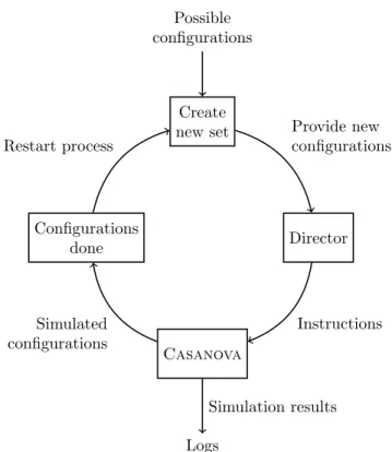
Galaxy Wars Lite (hereafter abbreviated as ‘GWL’) consists of various sepa-rately programmed components. These components are interdependent for run-ning simulations. How these components are related to one another, is displayed in figure 3.1.

Create new set Director Configurations done Casanova Possible configurations Logs Provide new configurations Instructions Simulated configurations Restart process Simulation results

Figure 3.1: GWL simulation cycle.

It is desirable to automate running consecutive simulations as much as pos-sible; it is not convenient having to run every simulation manually. Therefore, a Director script has been created in Python, with which _Casanova can be controlled. These controls are(i)setting the strategy for each AI,(ii) running multiple games sequentially, and(iii)logging. After post-processing tasks, the logs that are created through_Casanovalead to the case base.

The Director script itself is also dependent on input, which originates from an exhaustive list of all possible AI strategies competing against each other (henceforth referred to as ‘configurations’, see Subsection 3.2.1). This list is not influenced during simulations. The director script needs a batch of configura-tions that it has to carry out sequentially, which is provided by the ‘Create new set’-program. This program takes as input all possible configurations and the configurations that have been simulated, by which the configurations that are yet to be simulated can be derived. These un-simulated configurations are then loaded into the Director script, completing the cycle.

3.2.1

Strategy configurations

As has been mentioned, the simulation platform requires an exhaustive list of all possible AI configurations. Each strategy has a few properties. Every strategy

consists of six ‘strategy elements’: (i) build a Mine Station,(ii)build a Power Plant,(iii)build a Research Station,(iv)build a Shipyard,(v)build a Fighter, and(vi)build a Turret.

Casanovainterprets the setting of a strategy element as a ‘tendency’. This means that a strategy with a high value on the ‘build a Power Plant’-element, has a high tendency to build a Power Plant during the game. In this experiment, for every possible AI strategy, these six tendencies were ranked. A strategy can, as such, be regarded as an ordered priority list where values from 1 to 6 are distributed. Therefore, ‘123456’ and ‘314265’ would be, amongst many (i.e., 6!) others, valid strategies. Note that ranks in tendencies are merely ordinal: a strategic element ranked sixth does not necessarily trigger twice as frequently as an element ranked third. This implies that multiple simulations with equal tendency settings could return different results.

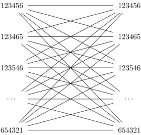
Since the case base requires the outcome of two strategies against each other, a list needed to be created containing all possible combinations of strategies. Figure 3.2 schematically displays the composition of these combinations.

Note: in similar research, a strategy like this is commonly referred to as ‘DNA sequence’, with its ‘genes’ being the separate settings. This thesis will also incorporate this terminology.

123456 123456

123465 123465

123546 123546

. . . .

654321 654321

Figure 3.2: Combinations of opposing AI strategies.

It results in valid combinations such as ‘123456+654321’ or ‘456123+523614’. The total number of opposing AI strategies is calculated by the formula given below.

O= (n!)

2_+n!

2

number of simulations to run can be calculated as:

O= (6!)

2_{+ 6!}

2 = 259560

3.2.2

Limitations

After a few random pilot tests, it became clear that each game lasted for a couple of minutes. In some cases, a simulation would even last indefinitely because two or more opposing Fighters would end their search for remaining enemy entities. As it was not possible to further modify game mechanics in_Casanova, a few global limitations had been applied:

(i) The total number of planets in the map was reduced to two (i.e., one ‘base’ planet for each AI). This forces every ship to cross only one mutual path.

(ii) Since it would still occur that only two opposing ships would remain on enemy territory, the maximum duration of a simulation was fixed to 50 game ticks. The result of this game can be interpreted as a draw.

(iii) As the simulations would only run in real-time, the average duration of one simulation in a pilot batch was about 3.5 minutes. This leads to a total simulation time of 259560×3.5 = 908460 minutes (i.e., 15141 hours, about 630 natural days, or almost 2 years). Since that would be far from feasible for this thesis project, the Research Facility was suppressed by fixing its rank in the order to 1. This led to the following number of simulations:

O= (5!)

2_{+ 5!}

2 = 7260 (i.e.,±18 natural days of total simulation time) As the platform would crash about once in every hundred simulations, it had to be restarted manually, and could therefore only run partially at night. Still, this was feasible for this project.

An alternative solution to this problem would have been not to run all possible simulations. In this research, a complete case base with one less input variable (being the Research Facility) was favoured over an incom-plete case base with one more input variable.

Note: with the Research Facility gone, the possibility of building Battle-ships is rendered moot.

During simulations, log files were created. These log files were processed into a case base, which states the configurations of both game AIs, how long the game lasted, and which AI won (or if the game ended in a draw). This case base can be put to use in various experiments, which will be specified in this section.

3.3

Experiment I: Fuzzy logic classification

This is not as straightforward as querying a complete case base on what AIs won against a given enemy strategy, and picking one of these winners as a counter for that enemy. It would be unwise to rely on one strategy that did win according to the case base, where that very instance could have been luck. It is more interesting to investigate what all the winning strategies had in common, i.e.: what tendencies were set relatively high or low, in order to achieve victory? In order to investigate this two steps had to be taken.

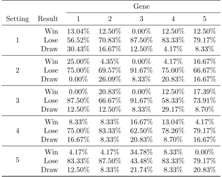
Firstly, the program searched the case base for all instances wherein the opposing strategy was simulated. In this project, these were 5! cases, as every strategy had 5 genes to adjust. The result was a table, stating which strategy gene, at which setting, ended up in which result (win, lose or draw). Since these tables were a translation from the case base, they are hereafter referred to as ‘case base tables’. To prevent mirrored matches (e.g. 12345 versus 12345) from bringing the chance-values in the case base table off balance, potential counters could not have the same strategy as their enemy. This lead to 5!−1 = 119 possible counters. Table 3.1 is an example of a case base table.

Subsequently, the performance of all AI configurations was measured by matching the setting of each of their genes against the case base table. These performance scores were used to determine what AI counter worked best. De-termining the best counter was done in three different ways. These three ap-proaches are described in the following paragraphs.

Gene Setting Result 1 2 3 4 5 1 Win 13.04% 12.50% 0.00% 12.50% 12.50% Lose 56.52% 70.83% 87.50% 83.33% 79.17% Draw 30.43% 16.67% 12.50% 4.17% 8.33% 2 Win 25.00% 4.35% 0.00% 4.17% 16.67% Lose 75.00% 69.57% 91.67% 75.00% 66.67% Draw 0.00% 26.09% 8.33% 20.83% 16.67% 3 Win 0.00% 20.83% 0.00% 12.50% 17.39% Lose 87.50% 66.67% 91.67% 58.33% 73.91% Draw 12.50% 12.50% 8.33% 29.17% 8.70% 4 Win 8.33% 8.33% 16.67% 13.04% 4.17% Lose 75.00% 83.33% 62.50% 78.26% 79.17% Draw 16.67% 8.33% 20.83% 8.70% 16.67% 5 Win 4.17% 4.17% 34.78% 8.33% 0.00% Lose 83.33% 87.50% 43.48% 83.33% 79.17% Draw 12.50% 8.33% 21.74% 8.33% 20.83% Table 3.1: Chance distribution of every option against enemy 12543 (except 12543 itself)

The maximum chance of winning approach considers every possible counter (5! possibilities with 5 genes, minus one because mirroring is not desired as ex-plained on page 15), and extracts the chance of winning for each of its settings from the case base table. Because the genes have a logical AND-relation, the overall winning chance of this strategy is the minimum of the winning chances (probabilities of winning, ‘PW’) of each individual gene. Python’s ’max()’-function determined what counter was ultimately chosen and returned only one counter in all cases. Official documentation does not specify how max() decides what value to return when two or more are highest. The algorithm, hereafter called ‘Max win’, for calculating the maximum winning chance (P W) is:

P W = max   

P WAI1= min(P Wgene1, P Wgene2, P Wgenei, P Wgene5)

P WAIn= min(P Wgene1, P Wgene2, P Wgenei, P Wgene5)

P WAI119 = min(P Wgene1, P Wgene2, P Wgenei, P Wgene5)

The minimum chance of losing is an alternative approach to calculating the highest chance of winning. The algorithm is based on the algorithm used for calculating the maximum chance on winning. The difference is that the algorithm identifies the weakest link in a strategy by the gene with the highest losing chance. The algorithm, hereafter called ‘Min lose’, for calculating the minimum losing chance (P L) is:

P L= min   

P LAI1= max(P Lgene1, P Lgene2, P Lgenei, P Lgene5)

P LAIn= max(P Lgene1, P Lgene2, P Lgenei, P Lgene5)

P LAI119 = max(P Lgene1, P Lgene2, P Lgenei, P Lgene5)

A mixed-mode approach is to also consider the chance on a draw. Beside calculating the winning chance of one gene’s setting, it also calculates the chance on a draw (P D) with that same setting. As the combination of winning and draw chances does not result in a pure winning chance, these combinations have been indicated by a plainP. The algorithm for calculating this score (hereafter referred to as ‘V-score’,V): V = max                                                PAI1 = min        (P Wgene1+ 0.5×P Dgene1), (P Wgene2+ 0.5×P Dgene2), (. . .), (P Wgene5+ 0.5×P Dgene5) PAIn = min        (P Wgene1+ 0.5×P Dgene1), (P Wgene2+ 0.5×P Dgene2), (. . .), (P Wgene5+ 0.5×P Dgene5) PAI119 = min        (P Wgene1+ 0.5×P Dgene1), (P Wgene2+ 0.5×P Dgene2), (. . .), (P Wgene5+ 0.5×P Dgene5)

All three algorithms provided the most powerful counter strategy possible against a given opposing strategy.

To see how strong the recommended counters from the algorithms are, more simulations needed to be run. Therefore, two experiments will were conducted: a quantitative and a qualitative experiment. In the quantitative experiment, the three fuzzy logic algorithms calculated the most fit counter against every possible combination. These configurations were simulated once to provide in-sight in how well the fuzzy logic algorithms work overall. For the qualitative experiment, 10 randomly picked enemies were matched against counters pro-vided by the three fuzzy logic algorithms. These combinations (30) were then simulated 20 times in _Casanova. The results of this qualitative experiment were analysed statistically.

Chance table

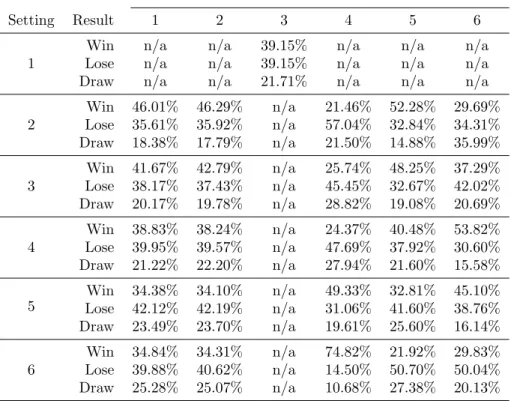
Similar to the case base table mentioned on page 15, a chance-table of every pos-sible match between combinations of AI strategies (7620 in total, as explained in Subsection 3.2.1) is displayed in Table 3.2. Although this table still incorporates six genes in a strategy (building a research facility was executed through gene 3; being fixed at setting 1), it gives a good overview of how settings on particular genes influence the chances of a certain outcome. For instance, it seems wise to have gene 4 on a relatively high setting, while the opposite is true for gene 5.

Gene

Setting Result 1 2 3 4 5 6

1

Win n/a n/a 39.15% n/a n/a n/a

Lose n/a n/a 39.15% n/a n/a n/a

Draw n/a n/a 21.71% n/a n/a n/a

2 Win 46.01% 46.29% n/a 21.46% 52.28% 29.69% Lose 35.61% 35.92% n/a 57.04% 32.84% 34.31% Draw 18.38% 17.79% n/a 21.50% 14.88% 35.99% 3 Win 41.67% 42.79% n/a 25.74% 48.25% 37.29% Lose 38.17% 37.43% n/a 45.45% 32.67% 42.02% Draw 20.17% 19.78% n/a 28.82% 19.08% 20.69% 4 Win 38.83% 38.24% n/a 24.37% 40.48% 53.82% Lose 39.95% 39.57% n/a 47.69% 37.92% 30.60% Draw 21.22% 22.20% n/a 27.94% 21.60% 15.58% 5 Win 34.38% 34.10% n/a 49.33% 32.81% 45.10% Lose 42.12% 42.19% n/a 31.06% 41.60% 38.76% Draw 23.49% 23.70% n/a 19.61% 25.60% 16.14% 6 Win 34.84% 34.31% n/a 74.82% 21.92% 29.83% Lose 39.88% 40.62% n/a 14.50% 50.70% 50.04% Draw 25.28% 25.07% n/a 10.68% 27.38% 20.13% Table 3.2: Chance distribution of all games in the case base

Table 3.2 also gives an indication of a baseline distribution of victories, losses and draws, because the research facility gene (3) was still incorporated in the table and has not being set other than 1. Gene 3 set at 1 (thus every strategy) has won and lost 39.15% of all played games. The number of games that ended in a draw being 21.71% indicates that 50 game ‘ticks’ per game to avoid long or even indefinitely lasting games was an appropriate choice.

3.4

Experiment II: Data mining

The goal of doing data mining experiments is to check what patterns in data lead to a certain result. The goal in this experiment is to check whether AI 1 or AI 2 wins, given their respective strategies. For the application of data mining techniques, Weka Experimenter 3.7.7 [18, 19] was used. This is a Java-driven, well-documented data mining tool that includes many important classifiers to model data with.

Weka handles .arff files, which is a file-type that contains various measure-ments (i.e., ‘attributes’, properties or features) over a number of instances. It might be convenient to imagine measurements and instances respectively as columns and rows. For this experiment, every game is represented as an in-stance and each strategy gene setting is represented as a measurement. This

way, the data file consists of the following measurements per instance:

(i) Tendencies of AI 1 to build a Power Plant, Mine Station, Research Facility, Shipyard, Turret or Fighter (6 in total);

(ii) Tendencies of AI 2 to build a Power Plant, Mine Station, Research Facility, Shipyard, Turret or Fighter (6 in total);

(iii) The winning AI.

The winning strategy of a game is indicated as a ‘class’ in an .arff file. Weka compares the value of class-measurements with all other measurements (thus, the settings of both AI players) using various techniques (i.e., classifiers). Each classifier (as illustrated in Section 2.3) outputs an ‘accuracy’ value, that repre-sents the number of correctly classified instances, taking into account previous measurements.

All experiments were conducted using the complete dataset. To prevent over-fitting (i.e., a well-trained classifier outputting a high accuracy, but only on the sample using in this experiment), ten-fold cross-validation were maintained. This technique allows a classifier to ‘see’ the actual class value related to certain measurements of 90% of the data (i.e., ‘train-set’), and then lets it classify the remaining 10% of the data (i.e., ‘test-set’). These classifications were then validated by checking the actual class-values, which returned an accuracy value. This was repeated 10 times in order to have all instances occur in a test-set once. Each classifier was built 10 times using the ten-fold cross-validation method. The average of these 10 accuracies is the actual accuracy for that classifier.

Chapter 4

Results

This result section provides the outcomes of the experiments conducted for this thesis project. In Section 4.1, both the quantitative and the qualitative fuzzy logic experiments will be covered. Section 4.2 will provide the results of all data mining experiments that were conducted to find a classifier giving the most accurate predictions on the case base. Additionally, Section 4.3 will illustrate a comparison between the prediction capabilities of the fuzzy logic algorithms and the strongest data mining classifier.

4.1

Fuzzy logic experiments

As stated in Section 3.3, three fuzzy logic-based algorithms (Max win, Min lose, and V-score) were programmed in order to recommend a counter strategy, based on a given enemy strategy. The program first maps a chance-table, based on the results of every possible configuration playing against the given enemy.

The three fuzzy logic algorithms process this chance-table and calculate which game AI has the most potential against the given enemy AI; all three algorithms have a different approach in determining this counter. To confirm if the predictions (see Section 4.3) of the algorithms were correct, two fuzzy logic experiments have been conducted.

The first experiment was a run through all possible strategies against the 3 counters recommended by the fuzzy algorithms. In the second experiment, 10 randomly picked strategies competed against 3 AIs recommended by the fuzzy algorithms, but this time 20 times for each configuration. The results of these experiments are respectively displayed in Tables 4.1 and 4.2.

Counter won Enemy won Draw

Max win 75.00% 15.00% 10.00%

Min lose 63.33% 16.67% 20.00%

V-score 64.17% 20.00% 15.83%

Averages 67.50% 17.22% 15.28%

Table 4.1: Overall-experiment outcomes

Table 4.1 shows the results of all possible strategies against three coun-ters determined by the fuzzy logic algorithms. This gives insight in how well the counters determined by the fuzzy logic algorithms perform generally, as dominant enemy strategies are now compensated. The Min lose and V-score algorithms score comparable, while the winning percentage of the Max win

al-gorithm is considerably higher. Note that because every configuration has been simulated once, no valid statistical analysis can be executed on these results.

The results of the qualitative experiment, are shown in Table 4.2.

Setup Experiment

Algorithm Enemy Counter N Wins Losses Draws Max win 25143 14523 60 96.67% 1.67% 1.67% 42135 12534 40 72.50% 12.50% 15.00% 12354 52413 40 67.50% 5.00% 27.50% 53214 15432 40 80.00% 17.50% 2.50% 52413 12534 40 25.00% 52.50% 22.50% 34152 12435 40 92.50% 0.00% 7.50% 13524 24513 20 65.00% 15.00% 20.00% 21543 23514 40 45.00% 35.00% 20.00% 15423 23514 60 26.67% 21.67% 51.67% 42153 31524 40 90.00% 7.50% 2.50% Min lose 25143 14523 60 96.67% 1.67% 1.67% 42135 14523 20 85.00% 10.00% 5.00% 12354 14523 20 80.00% 0.00% 20.00% 53214 14532 20 95.00% 5.00% 0.00% 52413 32541 20 40.00% 40.00% 20.00% 34152 34125 20 95.00% 0.00% 5.00% 13524 21534 20 50.00% 25.00% 25.00% 21543 31524 20 35.00% 45.00% 20.00% 15423 23514 60 26.67% 21.67% 51.67% 42153 41532 20 100.00% 0.00% 0.00% V-score 25143 14523 60 96.67% 1.67% 1.67% 42135 12534 40 72.50% 12.50% 15.00% 12354 52413 40 67.50% 5.00% 27.50% 53214 15432 40 80.00% 17.50% 2.50% 52413 12534 40 25.00% 52.50% 22.50% 34152 12435 40 92.50% 0.00% 7.50% 13524 14523 20 35.00% 45.00% 20.00% 21543 23514 40 45.00% 35.00% 20.00% 15423 23514 60 26.67% 21.67% 51.67% 42153 31524 40 90.00% 7.50% 2.50% Table 4.2: Results of the qualitative fuzzy logic experiments

In Table 4.2, the ‘Setup’ column shows which randomly picked enemy was matched against which counter determined by the fuzzy algorithms. The algo-rithms have a notable overlap in recommending counter strategies. For instance, all three algorithms recommended strategy 14523 against enemy strategy 25143. This configuration was therefore, actually, simulated 60 times. This overlap been

indicated in the ‘N’ column. The ‘Wins’, ‘Losses’ and ‘Draws’ columns display outcome averages of N simulations for their respective strategy configurations. The means of all outcomes per fuzzy algorithm have been displayed in Table 4.3.

Classifier Mean Median Std. Deviation

Max win 66.08% 70.00% 26.10%

Min lose 70.33% 82.50% 29.04% V-score 63.12% 70.00% 27.94% Averages 66.51% 74.17% 27.69% Table 4.3: Means of win-ratios

At the first glance, the means might come across as disappointing. Table 4.1 hinted that the percentages should have been around 75% for the Max win and Min lose algorithms, which was at first sight confirmed by Table 4.2 wherein is pointed out that the recommended counters won most experiments cogently.

However, looking at Table 4.3, these relatively low means could be explained by the large standard deviations of these means (around 25%). The fact that the median values are higher than the mean values, points out that there were more matches won than lost, and that the mean winning percentage is degraded by a few outlying configurations wherein the fuzzy algorithms lost a vast majority of the matches. This effect is visualised in Figure 4.1: the “Gained”-curve is an illustration of the gained surface under the “Average”-curve. It proves that high percentages occurred more often than low percentages.

Comparing just the means, the performance of the counters recommended by the V-score algorithm performed best; the Min lose algorithm the lowest. None of these means differed significantly. Comparing the medians, the Min lose algorithm seemed to provide the most reliably scoring counters.

0 1 2 3 0 10 20 30 40 50 60 70 80 90 100 Frequeny Winning percentage Max win × × × × × × × × × × × × × × × × × × × × × × Min lose + + + + + + + + + + + + + + + + + + + + + + V-score 2 2 2 2 2 2 2 2 2 2 2 2 2 2 2 2 2 2 2 2 2 2 Average Gained

Figure 4.1: Distribution of winning percentages

4.2

Data Mining experiment

Various data mining classifiers have been run over the dataset, and the resulting accuracies are shown in Table 4.4. The second column of this table shows the settings for each classifier that were changed from default to the given value. These settings are described in Section 2.3. The third column in the table below is the average accuracy of the classifier after running it 10 times.

Classifier (non-default) Settings Accuracy (non-default) Settings Accuracy ZeroR n/a 42.45 (0.06) IBk K = 1 53.18∗ (1.78) K = 24 67.43 (1.74) K = 5 64.56∗ _{(1.76) K = 25 67.43 (1.75)} K = 10 66.57∗ _{(1.63) K = 26 67.44}∗∗_(1.68) K = 15 66.92∗ (1.65) K = 27 67.37 (1.64) K = 16 67.00∗ (1.68) K = 28 67.34 (1.70) K = 17 67.03∗ (1.71) K = 29 67.24 (1.68) K = 18 67.11 (1.62) K = 30 67.16 (1.72) K = 19 67.32 (1.63) K = 31 67.09∗ (1.71) K = 20 67.32 (1.70) K = 32 67.06∗ (1.72) K = 21 67.34 (1.72) K = 33 67.10∗ (1.74) K = 22 67.38 (1.69) K = 34 67.09∗ (1.69) K = 23 67.42 (1.68) K = 35 67.05∗ (1.70) J48 C = 0.01 68.72∗ (1.75) C = 0.12 69.21 (1.59) C = 0.02 69.21 (1.75) C = 0.13 69.09 (1.59) C = 0.03 69.33 (1.68) C = 0.14 69.06 (1.64) C = 0.04 69.37 (1.71) C = 0.15 69.05 (1.66) C = 0.05 69.35 (1.71) C = 0.16 69.00∗ (1.65) C = 0.06 69.36 (1.68) C = 0.17 68.87∗ (1.64) C = 0.07 69.38∗∗ (1.77) C = 0.18 68.78∗ (1.62) C = 0.08 69.31 (1.71) C = 0.19 68.62∗ (1.64) C = 0.09 69.25 (1.65) C = 0.20 68.52∗ (1.66) C = 0.10 69.23 (1.63) C = 0.25 68.00∗ (1.57) C = 0.11 69.25 (1.60) MultiLayer Perceptron N = 50 67.02∗∗ (1.88) N = 5000 66.89 (1.83) N = 500 66.98 (1.80)

Table 4.4: Data mining results. Underlined: Optimal accuracy.

∗_{: Statistically different from optimal accuracy.}

∗∗_{: Statistically different from the optimal accuracies of other classifiers.}

Although the actual percentages from the experiment do not completely match the predicted percentages (see Section 4.3), there seems to be a relation between these scores. Where the expected percentage is relatively low, so is the percentage from the experiment and vice versa. In most cases, the actual percentage is higher than the expected percentage. The means of the winning percentages of each fuzzy logic algorithm are displayed in Table 4.3.

The J48 decision tree classifier scored the highest accuracy of 69.38%. As this accuracy is found using 10-fold cross-validation, this means that when the classifier is given 90% of the dataset, it can classify 69.38% of unseen cases

correctly.

The advantage of the decision tree scoring the highest, is that it visualises how the tree is constructed. This way, it is usable for other experiments, as has been done in order to compare its predicting power (see Section 4.3).

The accuracies of all four classifiers differed significantly. The accuracies of IBk and MLP differed the least. Details on statistical differences are available in Appendix A.

4.3

Predictions

All three fuzzy logic algorithms and the J48 classifier gave a prediction on how well the recommended counter would perform against a given enemy strategy. Note that all predictions are based on the potential performance of a counter that was provided by the fuzzy algorithms. These predictions, along with the outcome of the experiments, are displayed in Table 4.5.

Setup FL algorithms Algorithm Enemy Counter Baseline J48 Predicted Actual

Max win 25143 14523 48.74% 83.65% 54.17% 96.67% 42135 12534 53.78% 83.65% 60.87% 72.50% 12354 52413 45.38% 83.65% 52.17% 67.50% 53214 15432 34.45% 83.65% 41.67% 80.00% 52413 12534 11.76% 76.47% 16.67% 25.00% 34152 12435 68.91% 83.65% 75.00% 92.50% 13524 24513 19.33% 66.67% 20.83% 65.00% 21543 23514 13.45% 76.47% 16.67% 45.00% 15423 23514 7.56% 73.68%∗∗ 8.33% 26.67% 42153 31524 66.39% 83.65% 79.17% 90.00% Min lose 25143 14523 48.74% 83.65% 20.83%∗ 96.67% 42135 14523 53.78% 83.65% 16.67%∗ 85.00% 12354 14523 45.38% 83.65% 33.33%∗ 80.00% 53214 14532 34.45% 83.65% 45.83%∗ 95.00% 52413 32541 11.76% 66.17%∗∗ 79.17%∗ 40.00% 34152 34125 68.91% 71.60% 0.00%∗ 95.00% 13524 21534 19.33% 66.67% 60.87%∗ 50.00% 21543 31524 13.45% 66.17%∗∗ 70.83%∗ 35.00% 15423 23514 7.56% 73.68%∗∗ 79.17%∗ 26.67% 42153 41532 66.39% 83.65% 4.35%∗ 100.00% V-score 25143 14523 48.74% 83.65% 70.83% 95.00% 42135 12534 53.78% 83.65% 69.57% 72.50% 12354 52413 45.38% 83.65% 58.70% 67.50% 53214 15432 34.45% 83.65% 45.83% 80.00% 52413 12534 11.76% 76.47% 18.75% 25.00% 34152 12435 68.91% 83.65% 87.50% 92.50% 13524 14523 19.33% 66.67% 29.17% 35.00% 21543 23514 13.45% 76.47% 20.83% 45.00% 15423 23514 7.56% 73.68%∗∗ _{14.58% 20.00%} 42153 31524 66.39% 83.65% 85.42% 90.00% Table 4.5: Expected and actual winning chances for Counter

∗_{: Predicted losing chance}

∗∗_{: The chance the enemy would win; the J48 decision tree predicted a loss for}

The values in the Baseline column are averages of how well all possible configurations would perform against the enemy strategy. This way, relatively strong enemy strategies can be identified, which provides some perspective on other predictions.

The J48 decision tree that was constructed during the data mining experi-ment has been converted to a Python script that imitates the decisions of the J48 classifier. It takes both AI strategies as input, which are passed through numerous logical tests (e.g. “if AI gene 2 setting >3, then:”, etc.), and subse-quently returns the winning strategy along with the chance of that prediction being true. It should be noted that every J48 prediction is subject to an accu-racy of 69.38%; about 30% of all J48 classifications (determining the winner) on unknown cases, are false.

An important distinction should be made while interpreting the J48 “pre-dictions”. They should be considered a review of the counters recommended by the fuzzy logic algorithms: J48 does not recommend a counter, it merely provides a winning chance of an already recommended counter.

Note that predictions have only been made on winning chances. It has been chosen to do so, because the J48 classifier and the V-score fuzzy algorithm provide only a prediction of winning and “not winning”; information on the ratio of losing and games ending in a draw is rendered unknown by the mechanics of these methods. The same applies to the Min lose algorithm; when a chance on losing is given, the exact chance on winning (instead of “not losing”) is unknown. Therefore, not all classifiers and methods can be compared on losing- and draw chances.

4.3.1

Plots

A visual insight in the relations between predictions and actual scores, can given by plotting the data from Table 4.5 into a graph. Therefore, three plots (one plot per fuzzy algorithm) have been created to illustrate the relation between predictions and actual outcomes. These plots are displayed in Figures 4.2, 4.3, and 4.4.

0 20 40 60 80 100 1 2 3 4 5 6 7 8 9 10 Win percentage Configuration Actual × × × × × × × × × × × Fuzzy Logic H H H H H H H H H H H Baseline N N N N N N N N N N N J48 • • • • • • • • • •

Figure 4.2: Predictions Max win algorithm

0 20 40 60 80 100 1 2 3 4 5 6 7 8 9 10 Win percentage Configuration Actual × × × × × × × × × × × Baseline N N N N N N N N N N N J48 • • • • • • • •

0 20 40 60 80 100 1 2 3 4 5 6 7 8 9 10 Win percentage Configuration Actual × × × × × × × × × × × Fuzzy Logic H _H H H H H H H H H H Baseline N N N N N N N N N N N J48 • • • • • • • • • •

Figure 4.4: Predictions V-score algorithm

The actual winning chance typically lies between the predictions of the J48 classifier and the fuzzy logic algorithms, where the J48 predictions are the most optimistic. Which of the J48 or fuzzy algorithms predictions are the most accurate seems to depend on which fuzzy algorithm was used to generate the counter: in the Max win plot (Figure 4.2), 6 out of 9 J48 predictions were the closest to the actual outcome, where in the V-score plot (Figure 4.4) only 2 out of 9 J48 predictions were the more accurate than the fuzzy logic algorithm.

It is striking that the predictions of the fuzzy algorithms are relatively pes-simistic. This can be explained due to the fact that the fuzzy algorithms base their predictions on the most negative gene setting in the AND-relation that forms the strategy. For instance, if all genes in a strategy would cause a 95%+ winning chance except for one gene causing a 70% winning chance, the predic-tion of the Max win fuzzy algorithm would be based on this minimum.

The success of the J48 predictions can be explained due to the fact that they are merely judgements on counters that were already selected by the fuzzy algorithms (thus not providing suitable counters itself). Combined with the knowledge that fuzzy algorithms are designed to provide pessimistic predictions, it is only logical that J48 predictions are more accurate.

There are no fuzzy logic algorithm predictions in the Min lose plot (Fig-ure 4.3) because, as has been explained in Section 4.3, this algorithm predicts only chances on losing; not-losing is a combination of winning and ending in a draw, and as such, these values cannot be compared to J48 predictions. It should also be noted that no predictions of any kind fell below baseline.

4.3.2

Statistics

As explained in Section 4.3.1, comparing the predictability power of the J48 classifier and the fuzzy algorithms depends on which fuzzy algorithm recom-mended the counter. This has been done in Table 4.6. Additionally, the results of a comparison of all predictors regardless of which algorithm recommended the counter are displayed in the bottom rule of this table.

Predictors compared N Mean difference Std. Deviation Sig. (2-tailed) Max win Baseline - Actual 10 -29.11 12.80 .000∗

J48 - Actual 9 9.70 20.86 .200

Fuzzy - Actual 10 -23.53 13.71 .000∗

Min lose Baseline - Actual 10 -33.36 12.41 .000∗

J48 - Actual 9 -6.45 13.63 .257

V-score Baseline - Actual 10 -26.14 12.04 .000∗

J48 - Actual 9 13.00 21.84 .112

Fuzzy - Actual 10 -13.00 11.05 .005∗ Overall Baseline - Actual 30 -29.54 12.36 .000∗

J48 - Actual 27 6.37 20.47 .133

Fuzzy - Actual 20 -21.92 34.48 .002∗

Table 4.6: Predictors compared: paired t-tests

∗_{: Statistically different}

Comparing the actual outcomes with the predictions, the J48 predictions were the closest to the actual outcomes; the mean difference was found to be non-significant only for J48 predictions. As explained on page 29, this is not surprising; J48 merely did predictions on the potential of counters that were already selected by the fuzzy algorithms.

Note that the number of samples (N) is considerably low; 10 tests per fuzzy algorithm have been conducted. This means that when the number of samples would be higher, the difference between J48 predictions and the actual results may become significant. This becomes clear in the overall comparison: as more results are compared, the J48 predictions approach significance. Also, note that the predictions of the fuzzy algorithm were not incorporated in the Min lose comparison, as explained in Section 4.3.

Chapter 5

Discussion

For this thesis investigation, various experiments were conducted. The results of these experiments will be discussed in Section 5.1. The limitations of the ex-periments will be covered in Section 5.2. Section 5.3 provides recommendations for future research.

5.1

Discussing results

When designing the experiments, a chance table (Table 3.2) was generated in which every game AI strategy was matched up against any other possible strat-egy. As explained in Section 3.3, the baseline chances of winning and losing are both about 40%, and 20% for ending in a draw. It also became clear that there were dominant strategies: winning chances would improve if gene 4 was set at 5 or 6, or having gene 5 set at 2 or 3 (note that this table was generated while still maintaining 6 genes with 6 possible states). How the fuzzy logic algorithms and data mining classifiers performed with respect to these global baselines, is explained in the following paragraphs.

In the quantitative fuzzy logic experiment, every possible configuration was countered by a strategy recommended by all three fuzzy algorithms. The Max win algorithm scored highest with a victory-percentage of 75.00%, followed by the V-score algorithm (64.17%). Min lose scored the lowest: 63.33% of these counters were successful. Although these percentages give an overall insight into how well the various counters performed, no statistical conclusions could be drawn from these percentages.

Therefore, ten randomly picked strategies were to be countered twenty times by all three fuzzy algorithms. Here, the counters provided by the Min lose algo-rithm won an average of 70.33% the games, followed by Max win which scored 66.08%. V-score counters won the least of their matches: 63.12%. The medians of Max win, Min lose and V-score were 70.00%, 82.50% and 70.00% respec-tively, indicating that there were dominant enemy strategies that suppressed the average scores.

The accuracies of the trained classifiers in the data mining experiments, except for the ZeroR classifier, were all slightly below 70%. An explanation for this result is found in how the case base was built: every match was simulated only once, and it is plausible that some outcomes of these simulations were against the odds. As a result, the classifiers were potentially trained with non-representative data, suppressing the accuracy scores.

Predictions

After the counters were determined by all three fuzzy logic classifiers, predictions were done in various ways. A baseline prediction was done based on how many of all possible configurations would win against the randomly selected enemy strategy. The Max win and V-score fuzzy logic algorithms based their win-chances on the weakest gene in the counter. The Min lose algorithm based its chances on the gene with the highest chance of losing. After selecting a counter, the generated strategies were run through the J48 decision tree that was generated during the data mining experiments, which also returned a prediction.

5.2

Limitations

Designing and conduction this thesis research, some choices have been made. This led to some limitations in this research that should be mentioned. This section will list these limitations.

5.2.1

Case base

The case base (i.e. dataset) for this research has been built by running sim-ulations with the Casanova platform. This platform wrote log-files, which were then post-processed into a case base. Two important choices were made in building this case base.

Firstly, possible simulations were run only once. It could very well be that a dominant strategy had coincidentally lost against a weak strategy, which causes noise in the case base. Secondly, the action ‘tendencies’ (e.g. ‘build power plant’ or ‘build fighter’) were incrementally ranked. This means that for 5 actions, 5 different settings were maintained to determine a strategy. Therefore, combinations like 22555, 13344 or even 22222 (although in the case of tendencies, there is no difference between 11111 and 55555) were not simulated.

Probability-based fuzzy logic algorithms and data mining classifiers pro-cessed this case base. They still work with noisy or incomplete data, but their outputs (respectively case base-tables and models), are based on this data and should therefore be interpreted considering this matter. Fuzzy logic proved to be suitable handling this noisy data, as the algorithms were capable of considering the effect of each setting for each strategy gene.

5.2.2

The game

Some decisions have been made while designing the game to run the simulations on. A major difference in normal RTS games, is that normally, a player cannot see what his adversary is building (unless a player would send a scout unit). This effect is called ‘fog of war’; a ‘fog’ that conceals everything in the game world, except for what the units that are owned by the player can see. Fog of war has not been implemented in the game, and while recommending counters, the enemy’s strategy was known beforehand. However, as was pointed out in Section 2.1, deriving the strategy of an opponent is a task that has been successfully performed before.