CLAREMONT McKENNA COLLEGE
SCALABLE COLLABORATIVE FILTERING RECOMMENDATION ALGORITHMS ON APACHE SPARK
SUBMITTED TO
PROFESSOR DEANNA NEEDELL
AND
DEAN NICHOLAS WARNER
BY EVAN CASEY
FOR
SENIOR THESIS
SPRING 2014 28 APRIL 2014
Abstract
Collaborative filtering based recommender systems use information about a user’s preferences to make personalized predictions about content, such as topics, people, or products, that they might find relevant. As the volume of accessible information and active users on the Internet continues to grow, it becomes increasingly difficult to compute recommendations quickly and accurately over a large dataset. In this study, we will introduce an algorithmic framework built on top of Apache Spark for parallel computation of the neighborhood-based collaborative filtering problem, which allows the algorithm to scale linearly with a growing number of users. We also investigate several different variants of this technique including user and item-based recommendation approaches, correlation and vector-based similarity calculations, and selective down-sampling of user interactions. Finally, we provide an experimental comparison of these techniques on the MovieLens dataset consisting of 10 million movie ratings.
Contents
1 Introduction 5
1.1 Collaborative Filtering Based Recommender Systems . . . 5
1.2 Challenges Associated with Large-scale Collaborative Filtering . . . . 6
1.3 Collaborative Filtering in a Cluster Computing Environment . . . 7
1.4 Related Work . . . 8
1.5 Overview . . . 9
2 User-based Collaborative Filtering 11 2.1 Problem Statement . . . 11
2.2 Mathematical Formulation . . . 12
2.3 Sequential Algorithm . . . 13
2.4 Properties . . . 14
2.5 Item-based Collaborative Filtering . . . 15
3 Parallelized Implementation on Apache Spark 16 3.1 Introduction to Apache Spark . . . 16
3.2 Programming Model . . . 17
3.3 Algorithm . . . 19
3.3.1 Computing Item Similarities . . . 20
3.3.2 Computing the Top-N Recommendations . . . 22
3.4 Experimental Evaluation . . . 23
3.4.1 Speedup . . . 23
4 Variants of Neighborhood-based Collaborative Filtering 27
4.1 Parallel User-based Collaborative Filtering . . . 27
4.2 Similarity Measures . . . 28
4.3 Experimental Evaluation . . . 30
4.3.1 Mean Absolute Error . . . 30
4.3.2 Comparison . . . 31
5 Conclusion 33 5.1 Acknowledgments . . . 34
A Python Code for Parallel User-based Collaborative Filtering 35 B Python Code for Parallel Item-based Collaborative Filtering 42
Chapter 1
Introduction
1.1
Collaborative Filtering Based Recommender
Systems
The volume and diversity of information available on the web has grown exponentially in recent years in part due to the fact that modern web technologies have reduced the barrier to creating and distributing new information online. As a result of this, the content that is relevant to a particular user has become more specialized and harder to find.
Recommender systems aim to solve this problem by taking in a user’s past actions, such as articles they’ve read or products they’ve purchased and rated, to identify po-tential user preferences. Instead of providing a generic experience to every user, recommender systems personalize the experience of each user by surfacing content that is particularly relevant to their observed interests. If implemented correctly, recommender systems can be extremely effective at increasing engagement and pur-chasing. Today, many of the worlds most heavily trafficked websites, such as Netflix, LinkedIn, Amazon, and Twitter employ recommender systems to engage their users with relevant, personalized content.
In this study, we will focus on neighborhood-based collaborative filtering methods, which are a well-known technique used in recommender systems. Neighborhood-based collaborative filtering methods are item-based, meaning user preferences are inferred solely from what items the they and other users in the dataset have interacted with. As opposed to content-based methods, which incorporate descriptive or categorical data of each item into the model, neighborhood-based methods have the advantage of being able to incorporate new items easily, since each new item does not have to be classified into a specific genre or tied to a set of attributes. Furthermore, they provide results that are easily justifiable, since each user’s recommendations are derived from their own interaction history and the list of neighbor items or users.
1.2
Challenges Associated with Large-scale
Col-laborative Filtering
Due to the reasons outlined above, neighborhood-based methods are often preferred in large-scale, industrial use cases [5], even though other approaches can achieve higher prediction quality. As the size of the dataset grows, the scalability of neighborhood-based collaborative filtering recommender systems becomes essential.
However, neighborhood-based collaborative filtering is a memory-based approach, meaning that it utilizes the entire collection of every user’s interaction histories to generate predictions. As a result, they are highly computationally intensive and cannot scale to handle millions of users. Although most large-scale recommendations utilize an offline approach, in which the recommendations for each user in the dataset are computing all at once in a batch format, the application must be fast enough to compute new recommendations as users interest’s expand and evolve.
Moreover, large-scale recommender systems suffer from heavy-tailed item interac-tion distribuinterac-tions, wherein the most active users or ”power users” have an extensive item interaction history that is exponentially more than number of items in the
in-teraction history of an average user in the dataset. As a result, a disproportionate amount of computation is required to calculate their item recommendations, adding further complexity to the problem.
Lastly, the sparsity of large item sets that occurs as the number of items in the dataset grows can inhibit the accuracy of large-scale collaborative filtering recom-mender systems. In such systems, even the most active users may have interacted with less than 1% of the total number of items in the dataset. Certain items are inter-acted with more often, while others incur extremely few user interactions. As a result, recommendation accuracy suffers, since users share relatively fewer item interactions with one another.
1.3
Collaborative Filtering in a Cluster
Comput-ing Environment
Due to their data-intensive nature, recommender systems which employ neighborhood-based collaborative filtering methods are especially prone to scalability problems. Im-plementing such systems on one machine, although feasible, is disadvantageous from an efficiency and cost standpoint if the computational requirements of the system outpace the machine’s performance. Furthermore, it exposes the system to downtime risks if the machine fails. However, many of these problems can be solved by imple-menting recommender systems in a cluster computing environment via a distributed data processing framework such as Hadoop/MapReduce [3].
Implementing applications on a distributed data processing framework involves loading a driver program onto one machine, called the master node, which controls the execution of the program and data flow in the other machines in the cluster, called worker nodes. Each worker node in the cluster handles a small portion of the total computation in parallel with other worker nodes, thus improving the overall speed of computation for the program. By utilizing multiple machines, the risk of
downtime if a single machine in the cluster fails is eliminated due to the ability of other machines in the cluster to redistribute the work of the failed worker node. Moreover, the advent of cloud computing services such as Amazon Web Services enables machines to be rented temporarily on demand and added to the cluster at any time, allowing for seamless scalability if more computational power is needed. The low cost of renting virtual machines has served to further reduce the upfront cost of implementing large-scale, data intensize workflows and has contributed to the popularity of using cluster-computing for large-scale recommender systems
The technical approach for applying this to collaborative filtering methods, in-volves modifying the underlying algorithm to utilize the programming model specific to the data-processing platform in use. For example, the Hadoop framework imple-ments the MapReduce programming model, in which the user specifies a map function that processes a key/value pair to generate a set of intermediate key/value pairs and a reduce function that merges all intermediate values associated with the same in-termediate key. Once this is done, the underlying parallel processing platform uses a distributed file system to provide high throughput access to the data and manages the horizontal scalability of adding more machines to the cluster and dealing with machine failures.
1.4
Related Work
Neighborhood-based collaborative filtering methods are a well-known approach in academic literature to the problem of recommending relevant content to a user. Re-search has been devoted to investigating the use of different similarity metrics to measure the pairwise comparisons of users and items [1]. Research has also been done to address the problem of item interaction sparsity in a large dataset in the context of neighborhood models [5]. For example, certain methods, such as Latent Semantic Indexing (LSI), analyze the user-item representation matrix to identify re-lations between different items and the use these rere-lations to compute the prediction
score for a given user-item pair.
More recently, research on scalable collaborative filtering methods has shown that selective down-sampling of user interactions can improve the scalability of collabo-rative filtering algorithms with minimal effect on prediction quality. However, due to novelty of parallel processing tools and the ever-evolving nature of data-processing technology, there is limited research on collaborative filtering methods which utilize distributed computation. While prior work in this area has shown that it is possible to parallelize neighborhood-based collaborative filtering algorithms with MapReduce [4] [5] [9], MapReduce is not well-suited to expressing iterative, multi-stage algorithms and is relatively inefficient for such applications.
1.5
Overview
In this study, we propose an algorithmic framework for fast, scalable neighborhood-based collaborative filtering recommendations. We improve the scalability of the neighborhood-based collabortive filtering technique by implementing the underlying algorithm onSpark [8], a newly introduced distributed cluster computing system plat-form for efficient computation on large datasets, which, unlike Hadoop/MapReduce, is well-suited to the iterative, multi-step applications. The framework is open-source and is publicly available on GitHub, at https://github.com/evancasey/sparkler, under the MIT license.
Since no literature has been published so far on neighborhood-based collabora-tive filtering methods on Spark, this research seeks to investigate how Spark can be used to implement and improve the scalability of the well-known neighborhood-based collaborative filtering algorithm. This research builds off the ideas presented in imple-mentations of other machine learning algorithms on Spark, such as Alternating Least Squares [2] and Gradient Descent [6]. It also builds off of several ideas implemented in the MapReduce framework for item-based collaborative filtering presented by Schelter et al. [5], such as selective down sampling of power users and the use of a broadcast
variable to store the item similarity matrix, which will be discussed later on is this paper. While research has been done on scalable user-based collaborative filtering [9], there is even less research available on this method than the item-based variant. As a result, this study presents concepts that may be useful for future research on scalable user-based collaborative filtering methods.
In this paper, we provide the following contributions to the current body of re-search on scalable recommender systems:
• We introduce an algorithmic framework for efficient neighborhood-based col-laborative filtering on Apache Spark that scales linearly with a growing user base.
• We describe how to implement both user and item-based recommendation ap-proaches, as well as a variety of similarity measures, in an efficient manner using the high-level programming model provided by Apache Spark.
• We investigate the core differences underlying the Spark and Hadoop/MapReduce frameworks and discuss why Spark is especially efficient in certain cases.
• We present an experimental evaluation of the different recommendation and similarity methods on the Movielens dataset.
The rest of this paper is organized as follows: In section 2 we provide the reader with an introduction to the collaborative filtering problem and describe the algo-rithmic challenges it presents. In section 3 we describe Spark in detail and develop the item-based parallel algorithm. In section 4 we investigate the variants of this algorithm, including user-based recommendations and different similarity measures.
Chapter 2
User-based Collaborative Filtering
2.1
Problem Statement
In a typical collaborative filtering scenario, we have a list ofnitemsI ={i1, i2, ..., in}
and a list of k users U ={u1, u2, ..., uk}. Let M be a n×k matrix where each Mu,i
entry represents the rating score, or opinion, of a user u about an item i with its value being a real number or missing. The item iteraction history of a particular user
u is theu-th row ofM. The absence of a rating at a given Mu,i index occurs when a
user has not yet rated thei-th item. The task of the user-based collaborative filtering algorithm is to predict the items that will have the highest utility for a given user
u∈U based onu’s rating scores and the preferences of users with similar interaction histories to u. This idea is based on the notion that users with similar preferences will gain utility out of the same items and thus a user’s future preference toward a given item can be inferred from the opinions of that user’s nearest neighbors (the users with similar interaction histories).
2.2
Mathematical Formulation
The first step in the user-based collaborative filtering algorithm is to obtain M, the user-item ratings matrix. We obtainM by mapping over every user in our dataset and collecting the corresponding item and rating pairs of that user into a list representing that user’s item interaction history. We contruct M by aggregating each user’s item interaction list into a list of lists.
Once the ratings matrix, M, has been obtained, the second step is to compute the similarities between users and obtain each user’s nearest neighbors. The similarity between anyux, uy ∈M can be computed by a variety of different similarity measures
(which we investigate later on in this study), but we will use the popular cosine similarity method in this example which is calculated by the following equation:
sim(ux, uy) = P i∈Pux,uy rux,iruy,i r P i∈Pux,uy rux,i2 r P i∈Pux,uy ruy,i2 (2.1)
where Pux,uy represents the subset of items i ∈ I for which both users have rated,
rux,i is the rating of userux on itemiand ruy,i in the rating of useruy on itemi. The cosine similarity method applies Euclidean (L2) normalization to the user vectors, represented by ux anduy, which projects them onto the unit sphere. Their similarity
is then calculated by taking their dot product, which is the cosine of the angle between the points denoted by the vectors. Since the ratings of each user are positive, the output of cosine similarity in this case is bounded by [0,1].
After computing the similarity between every ux, uy ∈ U, the third step is to
calculate the predicted rating for each item that a given useru∈U has not yet rated. Again, a variety of approaches to computing the predicted ratings exist, but we will use the widely used weighted sums approach in this example, which is calculated by the following equation:
rux,i = ¯rux+ P uy∈Rux,i (ruy,i−r¯ux)sim(ux, uy) r P uy∈Rux,i sim(ux, uy) (2.2)
whereRux,i represents the subset of users uy ∈U other thanux that have rated item
i and ¯rux is the average item rating of user ux. The weighted sums approach takes the average of the ratings of the active user’s neighbors, and weights each of them according to the neighbor user’s similarity with the active user.
Lastly, we compute the top nitem recommendations for a given userux by finding
the n items i ∈ I with the highest predicted rating rux,i. Since the predicted rating measures our prediction for how relevant a particular item is to the active user, we pick out the top n highest scored items from the weighted sums calculation.
2.3
Sequential Algorithm
The standard sequential approach for computing the top n item recommendations for a single user u with cosine similarity and weighted sums is shown in Algorithm 1 below:
Algorithm 1Sequential user-based collaborative filtering approach with cosine sim-ilarity and weighted sums
1: Inputs:
• M, the user-item ratings matrix. Each Mu,i element represents a rating and
is either in N or empty.
• u, the user we’d like to compute recommendations for.
• n, the number of item recommendations to return, where n∈N.
• Sim(u, v), a user-defined function which computes the cosine similarity between two user vectors u and v. (2.1)
• W eightedSums(u, S) a user-defined function which computes the predicted rating for each item prediction for a given user u. (2.2)
• T opN Recommendations(Ru, n), a user-defined function which sorts the
scored predictions and outputs the top n highest ranked items.
2: Outputs:
3: for user v ∈ M do
4: if v 6=u then
5: Su,v ← Sim(u, v)
6: end if
7: for item i ∈M do
8: if u did not interact with ithen
9: Ru ←W eightedSums(u, i, Su,v) 10: end if 11: end for 12: end for 13: Ru(n) =T opN Recommendations(Ru, n)
2.4
Properties
User-based collaborative filtering has the benefit of being easily understandable, since its method for recommending items to a user is inspired by how we often discover new content in real life. The nearest neighbors in user-based collaborative filtering can be thought of as our friends or family who recommend movies, books, or items that they’ve personally interacted with and evaluated.
Under the sequential user-based collaborative filtering approach, we observe that the worst case time complexity of computing the topN recommendations for a given user is O(nk), where n is the number of items and k is the number of users in our user-item matrix,M. Although there are ways to reduce this time complexity even in the sequential approach, each additional user increases the complexity of computing recommendations for any given user by a factor of n. As more users are added to the dataset, it’s easy to see why the scalabality of user-based collaborative filtering becomes a serious issue.
Furthermore, in user-based collaborative filtering, computing recommendations for a new user requires recomputing the active user’s nearest neighbors over the entire set of users. In the context of a large-scale recommender system, this is a significant performance bottleneck since the total number of users k in the dataset is usually much higher than the number of items n.
2.5
Item-based Collaborative Filtering
Item-based collaborative filtering is a similar algorithm to user-based collaborative filtering which also uses the neighborhood approach for computing recommendations. In item-based collaborative filtering, the algorithm infers a user’s preferences by com-puting the most similar items to each item they have interacted with. The same similarity measures used in user-based approaches apply for item-based approaches, except the similarity between item pairs is calculated instead. Once the most similar items are found, we computed item recommendations via the weighted sums method as before, except the active user’s rating of each item and the similarity score of each neighbor item are used in place of the user similarity score and the item ratings of each neighbor user.
The advantage of this approach is that adding a new user to the system does not require recomputing the entire user similarity matrix, since the item similarities do not change with a new user. Once the item similarity matrix has been computed, item recommendations for a new user can be computed quickly, since only the weighted sums calculation is required to compute them. Moreover, since the relationships be-tween items tend to be relatively static, item-based collaborative filtering can provide recommendations of equal quality to the user-based approach with less online compu-tation [5]. For these reasons, item-based collaborative filtering is often the method of choice for large-scale commercial recommender systems. In the next section, we will discuss how to implement a parallelized version of the item-based approach. In section 4 we will also present a parallelized implementation of the user-based approach.
Chapter 3
Parallelized Implementation on
Apache Spark
3.1
Introduction to Apache Spark
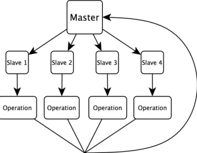
Apache Spark is a fast and general-purpose cluster computing system similar to the Hadoop data-processing platform that was originally developed in the AMPLab at UC Berkeley [7] [8]. Similar to Hadoop, Spark is built on top of the Hadoop Distributed File System, but unlike Hadoop it is not tied to an acyclic dataflow model such as MapReduce or Dryad. Instead, Spark utilizes a cyclic dataflow model in which the output of each parallel operation is cached in memory on each machine in the cluster. At each stage of the algorithm, the cached data can be accessed directly without having to repeatedly read from the file system or the master node.
The dataflow model of a single parallel operation in Spark is illustrated in figure 3-1 below. By caching the data in memory on each worker node, Spark ultimately reduces amount of data being passed over the network and as result is especially well-suited to iterative algorithms which reuse a working set of data across multiple parallel algorithms. In these circumstances, the reduced amount of data passed over the network enables Spark applications to run significantly faster when compared
to disk-based implementations on Hadoop [2]. In certain cases, Spark applications have achieved up to a 10x speed increase over Hadoop, although this result is highly dependent on the nature of the underlying algorithm.
Figure 3-1: Illustration of the Data Flow in Spark
As a biproduct of Spark’s data flow model, iterative algorithms that cannot be expressed well in the two-stage MapReduce programming model are more easily im-plemented on Spark. Furthermore, the use of in-memory caching of partitioned data on each worker node enables fast, interactive analysis of big datasets. Frameworks such as Pig and Hive, which are built on top of Hadoop and used to perform ad-hoc exploratory data analysis, incur significant latency when compared to Spark from having to read data from disk with each MapReduce job.
3.2
Programming Model
Implementing parallel programs in Spark is accomplished through the use of a driver program that runs on the master node of a Spark cluster and is responsible for express-ing the high-level control flow of a Spark job. Within a driver program, a Spark user defines a series of operations, such asmap,reduce, andfilter, which are executed on
each of the worker nodes in the cluster. This dataflow programming model is accom-plished through the use of several core abstractions provided by the Spark framework, most notably resilient distributed datasets, parallel operations, and shared variables, which we will discuss in detail below.
The resilient distributed dataset (RDD) is a read-only collection of objects par-tioned across a set of machines that can be rebuilt if a partition is lost. In a Spark program, data is first read in from a distributed file system, such as the Hadoop Dis-tributed File System (HDFS), into an RDD object. The RDD is then parallelized by the driver program, causing it to be partitioned and sent to multiple nodes. RDDs are lazy and ephemeral by default, meaning that the data in each partition only be-comes available when used in a parallel operation and is discarded from memory after use. However, for data that is intended to be reused later on in the algorithm, the persistence on an RDD can be altered by the use of a cache action, which advises Spark to keep the RDD in memory of the worker nodes to improve performance.
Once data has been read into an RDD, the initialized RDD can be transformed by applying parallel operations to it. For example, a parallel operation might be used to pass each element in an RDD object through a user-defined function via the map
operation. If the user-defined function transforms values of type X to values of type Y, then each element in the RDD will consist of values of type Y after the operation is applied. Spark offers a number of different parallel operations which can be applied on RDDs, but we will discuss only a few of them here which are relevant to the collaborative filtering algorithm. These include:
• map
Passes each element in the RDD through a user-defined function. Each element in the resulting RDD is the output of this function applied on the element in the original RDD
• filter
returns a boolean value. Each element in the resulting RDD is made up of elements in the original RDD for which the predicate function returns True.
• groupByKey
Aggregates the elements in an RDD based on the key of each element. When called on an RDD consisting of (K,v) pairs, returns all (K,Seq[V]) pairs where each key in the resulting RDD is unique.
• collect
Sends all elements in the RDD to the driver program, to be used when user wants to collect the results in the master node.
Lastly, Spark also enables the use of shared variables, such as broadcast and ac-culumulator variables for accessing or updating shared data accross worker nodes. Shared variables are copied to each worker node, and no updates to the variables on those nodes are propagated back to the driver program. In specific, if a large read-only piece of data is accessed in multiple parallel operations, using a broadcast variable is more efficient than storing that data in a read-write variable across tasks, since the data associated with that object is ensured to be only shipped to each worker once. Although the data in a parallelized RDD object is cached on each worker node already, the use of a broadcast variable prevents having to package the data stored in it with every task, thus increasing the efficiency of the Spark application.
3.3
Algorithm
In this section we will describe the implementation of item-based collaborative filter-ing on Spark. As described in Figure 3-2, the algorithm is made up of two separate components, item similarity computation and top n recommendations computation. The item similarity computation is executed first, followed by the top n recommen-dation computation. Since the top n recommendation computation uses the output of the item similarity computation, we initialize a broadcast variable to efficiently
embed the user similarity matrix in each worker node.
Figure 3-2: Diagram of Item-based Collaborative Filtering on Spark
3.3.1
Computing Item Similarities
Similar to the sequential approach, the first step in the parallel user similarity com-putation is to obtain M, the user-item ratings matrix. In this case, we initialize a
SparkContext object and use Spark’s textFile operation to read in the data from Amazon S3 into parallelized collection, specifying the number of partitions to dis-tribute the data across. We then construct M by mapping over every item in our dataset and collecting the corresponding user and rating pairs of that item. We then call cache to advise Spark to keep the RDD in memory of the worker nodes for improved performance. The rest of the item similarity computation proceeds below:
Algorithm 2Parallel Item Similarity Computation
1: Inputs:
• Mu,∗, an RDD representing the user-item ratings matrix, keyed on the user
index. Each Mu,∗ element represents a rating and is either in Nor empty.
• Sim(((u, v), Seq(V))), a user-defined function which computes the cosine similarity between two users uand v. V is a list of item-rating pairs for which
u and v have both interacetd with (2.1).
• SampleInteractions(K, Seq(V), n), a user-defined function which applies selective down sampling to Seq(V), a sequence of items. If the length of
Seq(V) exceedsn, the resulting value is a sample ofn items fromSeq(V).
• KeyOnF irstItem(((u, v), V)), a user-defined function which converts the key from (u, v) to u and appends v to the front of the value V resulting in a (u, V) tuple. This is used to to key pairwise objects on a single item.
• N earestN eighbors(K, Seq(V), k), a user-defined function that takes in the list of neighbor items to K, and outputs the k items with the highest
similarity to K.
• M ap(f,(K, V)), F ilter(f,(K, V)), and GroupByKey((K, V)) as defined previously, where (K, V) denotes an RDD object and f is a user-defined function.
2: Outputs:
• Su,v, the sparse user similarity matrix. Each Su,v element is either in [0,1]
or empty.
3:
4: function pairwiseItems(M, n)
5: itemRatingP airs←M ap(F indItemP airs(), M ap(SampleInteractions(n), Mu,∗)))
6: pairwiseItems←GroupByKey(itemRatingP airs)
7: emit pairwiseItems
8: end function
9:
10: function itemSimilaity(pairwiseItems, k)
11: itemSims←M ap(KeyOnF irstItem(), M ap(Sim(), pairwiseItems)
12: nearestItems←map(N earestN eighbors(k), GroupByKey(itemSims))
13: emit nearestItems
3.3.2
Computing the Top-N Recommendations
Once the item similarity matrix has been computed, the next step is to compute the top n recommendations for each user. This is done by iterating through the item interaction history of each user and computing the weighted sums score for each item’s neighbor items. In order to efficiently access the item similarity matrix, we call broadcast on the output of the parallel item similarity computation and pass this variable, nearestItems into the parallel top n recommendation function as a parameter. By storing the item interaction history as a broadcast variable, we reduce the amount of data being transmitted over the network. The top n recommendation computation is described in Algorithm 3 below:
Algorithm 3Parallel Top N Recommendations Computation
1: Inputs:
• Mu,∗, an RDD representing the user-item ratings matrix, keyed on the user
index. Each Mu,∗ element represents a rating and is either in Nor empty.
• nearestItems, the top k similar items for each item inM, as described in Algorithm 2. This variable is initialized as a broadcast variable.
• n, the number of item recommendations to return.
• W eightedSums(K, V, N earestItems, n), a user-defined function that
computes the item recommendations for each user K using the weighted sums approach (2.2).
• M ap(f,(K, V)) and GroupByKey((K, V)) as defined previously, where (K, V) denotes an RDD object and f is a user-defined function.
2: Outputs:
• itemRecs, the top n item recommendations for the active useru.
3: 4: function GroupedItemRatings(M) 5: U serItemRatings ←GroupByKey(Mu,∗) 6: emit U serItemRatings 7: end function 8:
9: function TopNRecommendations(U serItemRatings, N earestItems, n) 10: ItemRecs ←M ap(W eightedSums(N earestItems, n), U serItemRatings)
11: emit ItemRecs
3.4
Experimental Evaluation
In this section we present the results of an experimental evaluation of our parallel algorithm on a large dataset. We first evaluate the parallel algorithm on a local ma-chine running Spark 0.8.1 with one 4-core CPU, 16gb of memory, and one 128gb SSD. We find that the speedup increases linearly at first, but diminishes as the application becomes bottlenecked by network bandwith with more partitions. Next, we rented a cluster of m1.xlarge instances from Amazon Web Services, each running Spark 0.8.1 with 15gb of memory and eight virtual cores each, and show the linear speedup with a growing number of machines. In both experiments, we used the MovieLens 10M dataset, consisting of 10 million ratings applied to 10,000 movies from 72,000 users.
3.4.1
Speedup
For the experiments on a local machine, we ran the Spark application in local mode and measured the runtime as we increased the number of data partitions α, or nodes in the cluster. Each time we run the algorithm, we specify α, which Spark uses to determine the number of nodes to distribute the work across. On a single machine, Spark sets this value to the total number of available cores in the machine ifαexceeds this value.
In order to measure the performance of the parallel algorithm, we denote Tα as
the average runtime of the algorithm with α data partitions, and Ts as the baseline
speed for the algorithm with one data partition. We define the speedup with respect toα as follows:
Speedup= Tα
Ts
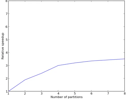
In Figure 3-3, our results show that increasing the number of partitions achieves linear speedup from 1 to 2 partitions, but then incurs diminishing speedup across
more partitions. From monitoring the system utilization during runtime, we find that this is due to network limitations of running Spark programs on one machine. As the number of partitions grows, the program becomes I/O bound, meaning that it’s speed is limited by the speed of input/output operations on that machine. After 4 partitions, we observe that the rate of speedup dramatically decreases, since Spark has expended the number of available cores on the machine.
Figure 3-3: Speedup for a growing number of partitions on one machine
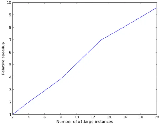
Despite the limitation of running Spark applications on a single machine, our ex-periments on a cluster of m1.xlarge instances on Amazon Web Services yielded much more favorable results. For these experiments, we used the Amazon ElasticMapRe-duce computing infrastructure to run our algorithm on a cluster of m1.xlarge ma-chines. We repeatedly ran the item-based collaborative filtering algorithm with an increasing number of clusters and observed the runtime complexity of the algorithm. However, as opposed to the case of a standalone Spark cluster, we define Ts as the
order to factor in the fixed cost of initializing the Spark cluster on Amazon Elastic MapReduce. Figure 3-4 shows the linear speedup of the item-based collaborative filtering algorithm with a growing number of machines.
Figure 3-4: Speedup for a growing number of machines in Amazon EC2
3.4.2
Optimizations
In order to achieve the linear speedup with the number of machines, we limited the item similarity computation to compute the 50 most similar items per item, which helps limit the search space for computing the top n most similar items. This is a common approach in academic literature, and has been shown to have a trivial effect on rating prediction quality ifnis set substantially high [1]. We also applied selective down sampling of item interactions, as presented in the work of Schelter et. al [5], to limit the number of items in the interaction histories of power users. We set p, the size of the interaction cut off, to 500, which is above the p >400 mark that Schelter
Chapter 4
Variants of Neighborhood-based
Collaborative Filtering
4.1
Parallel User-based Collaborative Filtering
In this section we will discuss how to implement user-based collaborative filtering on Spark. The user-based approach, like the item-based approach is split up into two main components, the user similarity computation and the top n recommendation computation. The user similarity computation is essentially identical to item sim-ilarity computation in item-based collaborative filtering, except that the algorithm computes pairwiseU sers instead of pairwiseItems and the Sim function computes the similarity between users instead of items.
When computing the topn recommendations with user-based collaborative filter-ing, item recommendations are generated by searching through the item interaction history of each neighbor user to the active user. This differs from the item-based ap-proach, in which we generate item recommendations from the neighbor items of each item the active user has interacted with. As a result of this, we initialize a broadcast variable to store the item interaction histories of each user in the dataset which we use to fetch the item interaction history of each of the active user’s neighbor users. Again,
this differs from the item-based approach where we broadcasted the item similarity matrix. The top nrecommendation algorithm for user-based collaborative filtering is described in Algorithm 4 below:
Algorithm 4 Parallel Top N Recommendations Computation for User-based Col-laborative Filtering
1: Inputs:
• M∗,i, an RDD representing the user-item ratings matrix, keyed on the item
index. Each Mu,∗ element represents a rating and is either in Nor empty.
• nearestU sers, an RDD representing the top k similar users for each user in
M.
• groupedU serRatings, the item interaction history for each user in M. This object is initialized as a broadcast variable.
• n, the number of item recommendations to return.
• W eightedSums(K, V, N earestU sers, n), a user-defined function that
computes the item recommendations for each user K using the weighted sums approach (2.2).
• M ap(f,(K, V)) and GroupByKey((K, V)) as defined previously, where (K, V) denotes an RDD object and f is a user-defined function.
2: Outputs:
• itemRecs, the top n item recommendations for the active useru.
3:
4: function TopNRecommendations(nearestU sers, groupedU serRatings, n)
5: ItemRecs ←M ap(W eightedSums(groupedU serRatings, n), nearestU sers)
6: emit ItemRecs
7: end function
4.2
Similarity Measures
In both item-based and user-based approaches, different notions of similarity can be used when computing the user or item similarity matrix. While there is no perfect similarity measure, certain datasets can be especially suited towards a particular similarity measure depending on factors such as rating scale and distribution or if the dataset consists of explicit/implicit feedback. In this section we will describe three of the most commonly used similarity measures besides cosine similarity, which include adjusted cosine similarity, Pearson correlation, and Jaccard similarity. The following descriptions of each similarity measure will be phrased in the context of user-based
collaborative filtering, as in Section 2.
The first of these similarity metrics is adjusted cosine similarity, which, similar to cosine similarity, is measured by normalizing the user vectors ux and uy and
com-puting the cosine of the angle between them. However, unlike cosine similarity, when computing the dot product of the two user vectors, adjusted cosine similarity uses the deviation between each of the user’s item ratings, denoted ru, and their average
item rating, denoted ¯ru, in place of the user’s raw item rating. In equation form, the
adjusted cosine similarity computation is expressed as:
sim(ux, uy) = P i∈Pux,uy (rux,i−r¯ux)(ruy,i−¯ruy) r P i∈Pux,uy (rux,i−r¯ux) 2r P i∈Pux,uy (ruy,i−¯ruy) 2 (4.1)
where Pux,uy represents the subset of items i ∈ I for which both users have rated,
rux,i is the rating of userux on itemiand ruy,i in the rating of useruy on itemi. The main advantage of this approach is that in item-based collaborative filtering, the item vectors consist of ratings from different users who often have varying rating scales.
Another approach to measuring similarity is the Pearson correlation coefficient. Like adjusted cosine similarity, Pearson correlation is concerned with accounting for changes in the rating scale across users and items. However, instead of using the difference between the user’s rating ru of an item and their average item rating ¯ru,
Pearson correlation takes the deviation between ru and ¯ri, the average of all ratings
for that item. In equation form, the Pearson correlation coefficient computation is expressed as: sim(ux, uy) = P i∈Pux,uy (rux,i−r¯i)(ruy,i−¯ri) r P i∈Pux,uy (rux,i−r¯i)2 r P i∈Pux,uy (ruy,i−r¯i)2 (4.2)
where Pux,uy represents the subset of items i ∈ I for which both users have rated,
represents the average rating of all users u∈U oni.
In many cases, the implicit feedback of a user-item interaction, that is, whether or not a user interacted with an item at all, can provide valuable information about a user’s preferences. The Jaccard similarity is one such measure that uses this infor-mation when measuring similarity across user or item vectors. In equation form, the Jaccard similarity computation is expressed as:
sim(ux, uy) =
|rux ∩ruy|
|rux ∪ruy|
(4.3)
whererux∩ruy is the number of items whichux and uy have both rated, andrux∪ruy is the total number of items collectively rated by ux and uy. Jaccard similarity has
the advantage of being easily computed and applicable for cases in which explicit feedback, such as ratings, are not available.
4.3
Experimental Evaluation
In this section we present the results of an experimental evaluation of the different similarity measures as described above. We compare the accuracy of the item-based collaborative filtering algorithm with each similarity measure on the MovieLens 10M dataset. As in the evaluation of parallel item-based collaborative filtering, we apply an interaction cut of p= 500 and use the top 50 most similar items for each item in the topn recommendations stage.
4.3.1
Mean Absolute Error
For evaluating the accuracy of the item recommendations computed by item-based collaborative filtering, we use Mean Absolute Error (MAE), a popular evaluation metric for collaborative filtering algorithms. Mean Absolute Error is a measure of the deviation of the predicted rating of an item by a user from the actual rating specified
by the user. We compute MAE by taking the average of these deviations for every item in the user’s interaction history, for each user in U. In equation form, MAE is expressed as: M AE = P i∈N |pi−qi| N (4.4)
where pi is the predicted rating of the item i computed by the collaborative filtering
algorithm, and qi is the actual rating of the item i specified by the user. The lower
the MAE, the more accurate the collaborative filtering algorithm is at predicting the item preferences of each user.
4.3.2
Comparison
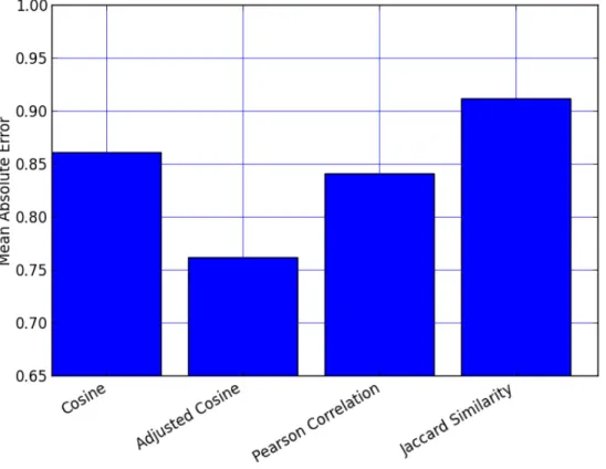
In order to compute the accuracy of each similarity measure in the item-based col-laborative filtering algorithm, we split the dataset into a training set and test set and compare the predicted item ratings computed by running the algorithm on the training set with the actual user-specified item ratings in the test. We construct the training and test sets by randomly partitioning the item ratings of each user with a training/test ratio of .9. That is, the item interaction history of each user in the training and tests sets is a random sample of their item ratings from the original dataset, but 90% of them appear in the training set and the remaining 10% appear in the test set. Figure 4-1 shows the results of effect of each similarity measure on the accuracy of the item-based collaborative filtering algorithm.
By comparing the resulting MAE of the item-based collaborative filtering al-gorithm between these similarity measures, we find that adjusted cosine similarity achieves the highest accuracy, with an MAE of .762. We also find that Pearson correlation achieves the second highest accuracy with an MAE of .841.
Figure 4-1: Impact of Similarity Metric on Item-based Collaborative Filtering Accu-racy
Chapter 5
Conclusion
In this study we illustrated how to build a scalable neighborhood-based collaborative filtering recommender system on Apache Spark. We provided the reader with an understanding of neighborhood-based collaborative filtering methods and discussed the challenges of implementing them at scale. We introduced the core concepts behind Spark’s novel data flow programming model and provided implementations of both user and item-based collaborative filtering algorithms on it.
Using a large dataset consisting of 10 million ratings, we provided an experimental evaluation of neighborhood-based collaborative filtering on Apache Spark and showed computational speedup that scales linearly with a growing number of machines. We discussed how optimizations such as selective down sampling of item interactions and neighborhood size can be applied to improve runtime performance. Finally, we compared several correlation and vector based similarity metrics and evaluated their effects on prediction quality.
In future work, we hope to investigate how Spark can be leveraged for a diverse set of collaborative filtering applications, such as online recommender systems and content-based approaches. Since there are many ways to customize collaborative filtering algorithms on a distributed data processing framework, it is hard to determine from academic literature exactly how the framework presented here compares with
similar Hadoop-based frameworks. Future research may uncover which framework is ideally suited for the neighborhood-based collaborative filtering algorithm.
5.1
Acknowledgments
I would like to thank Professor Deanna Needell for her guidance, support, and encour-agement as my advisor for this project. I would also like to thank Shawn Shah for his help in conceiving the idea for this project and providing crucial advice throughout the progression of this project. A special thanks to the CMC mathematics depart-ment for providing me with the resources and knowledge to understand and apply mathematics at a deeper level. Finally, a special thanks to my parents and sister for all of their support and love over the years.
Appendix A
Python Code for Parallel
User-based Collaborative Filtering
# User-based Collaborative Filtering on pySpark with cosine similarity # and weighted sums
import sys
from collections import defaultdict from itertools import combinations import random
import numpy as np import pdb
from pyspark import SparkContext def parseVectorOnUser(line):
’’’
Parse each line of the specified data file, assuming a "|" delimiter. Key is user_id, converts each rating to a float.
’’’
line = line.split("|")
return line[0],(line[1],float(line[2])) def parseVectorOnItem(line):
’’’
Parse each line of the specified data file, assuming a "|" delimiter. Key is item_id, converts each rating to a float.
’’’
line = line.split("|")
return line[1],(line[0],float(line[2]))
def sampleInteractions(item_id,users_with_rating,n): ’’’
For items with # interactions > n, replace their interaction history with a sample of n users_with_rating
’’’
if len(users_with_rating) > n:
return item_id, random.sample(users_with_rating,n) else:
return item_id, users_with_rating def findUserPairs(item_id,users_with_rating):
’’’
For each item, find all user-user pairs combos. (i.e. users with the same item) ’’’
for user1,user2 in combinations(users_with_rating,2): return (user1[0],user2[0]),(user1[1],user2[1]) def calcSim(user_pair,rating_pairs):
’’’
For each user-user pair, return the specified similarity measure, along with co_raters_count.
’’’
sum_xx, sum_xy, sum_yy, sum_x, sum_y, n = (0.0, 0.0, 0.0, 0.0, 0.0, 0) for rating_pair in rating_pairs:
sum_xx += np.float(rating_pair[0]) * np.float(rating_pair[0]) sum_yy += np.float(rating_pair[1]) * np.float(rating_pair[1]) sum_xy += np.float(rating_pair[0]) * np.float(rating_pair[1]) # sum_y += rt[1]
# sum_x += rt[0] n += 1
cos_sim = cosine(sum_xy,np.sqrt(sum_xx),np.sqrt(sum_yy)) return user_pair, (cos_sim,n)
def cosine(dot_product,rating_norm_squared,rating2_norm_squared): ’’’
The cosine between two vectors A, B
dotProduct(A, B) / (norm(A) * norm(B)) ’’’
numerator = dot_product
denominator = rating_norm_squared * rating2_norm_squared
return (numerator / (float(denominator))) if denominator else 0.0 def keyOnFirstUser(user_pair,item_sim_data):
’’’
’’’
(user1_id,user2_id) = user_pair
return user1_id,(user2_id,item_sim_data) def nearestNeighbors(user,users_and_sims,n):
’’’
Sort the predictions list by similarity and select the top-N neighbors ’’’
users_and_sims.sort(key=lambda x: x[1][0],reverse=True) return user, users_and_sims[:n]
def topNRecommendations(user_id,user_sims,users_with_rating,n): ’’’
Calculate the top-N item recommendations for each user using the weighted sums method
’’’
# initialize dicts to store the score of each individual item, # since an item can exist in more than one item neighborhood totals = defaultdict(int)
sim_sums = defaultdict(int)
for (neighbor,(sim,count)) in user_sims:
# lookup the item predictions for this neighbor
unscored_items = users_with_rating.get(neighbor,None) if unscored_items:
for (item,rating) in unscored_items: if neighbor != item:
# update totals and sim_sums with the rating data totals[neighbor] += sim * rating
sim_sums[neighbor] += sim # create the normalized list of scored items
scored_items = [(total/sim_sums[item],item) for item,total in totals.items()] # sort the scored items in ascending order
scored_items.sort(reverse=True) # take out the item score
ranked_items = [x[1] for x in scored_items] return user_id,ranked_items[:n]
if __name__ == "__main__": if len(sys.argv) < 3:
print >> sys.stderr, \
"Usage: PythonUserCF <master> <file>" exit(-1)
sc = SparkContext(sys.argv[1],"PythonUserItemCF") lines = sc.textFile(sys.argv[2])
’’’
Obtain the sparse item-user matrix:
item_id -> ((user_1,rating),(user2,rating)) ’’’
lambda p: sampleInteractions(p[0],p[1],500)).cache() ’’’
Get all item-item pair combos:
(user1_id,user2_id) -> [(rating1,rating2), (rating1,rating2), (rating1,rating2), ...] ’’’ pairwise_users = item_user_pairs.filter( lambda p: len(p[1]) > 1).map(
lambda p: findUserPairs(p[0],p[1])).groupByKey() ’’’
Calculate the cosine similarity for each user pair and select the top-N nearest neighbors:
(user1,user2) -> (similarity,co_raters_count) ’’’ user_sims = pairwise_users.map( lambda p: calcSim(p[0],p[1])).map( lambda p: keyOnFirstUser(p[0],p[1])).groupByKey().map( lambda p: nearestNeighbors(p[0],p[1],50)) ’’’
Obtain the the item history for each user and store it as a broadcast variable user_id -> [(item_id_1, rating_1),
[(item_id_2, rating_2), ...]
user_item_hist = lines.map(parseVectorOnUser).groupByKey().collect() ui_dict = {}
for (user,items) in user_item_hist: ui_dict[user] = items
uib = sc.broadcast(ui_dict) ’’’
Calculate the top-N item recommendations for each user user_id -> [item1,item2,item3,...]
’’’
user_item_recs = user_sims.map(
Appendix B
Python Code for Parallel
Item-based Collaborative Filtering
# Item-based Collaborative Filtering on pySpark with cosine similarity # and weighted sums
import sys
from collections import defaultdict from itertools import combinations import numpy as np
import random import csv import pdb
from pyspark import SparkContext
from recsys.evaluation.prediction import MAE def parseVector(line):
’’’
Converts each rating to a float ’’’ line = line.split("|") return line[0],(line[1],float(line[2])) def sampleInteractions(user_id,items_with_rating,n): ’’’
For users with # interactions > n, replace their interaction history with a sample of n items_with_rating
’’’
if len(items_with_rating) > n:
return user_id, random.sample(items_with_rating,n) else:
return user_id, items_with_rating def findItemPairs(user_id,items_with_rating):
’’’
For each user, find all item-item pairs combos. (i.e. items with the same user) ’’’
for item1,item2 in combinations(items_with_rating,2): return (item1[0],item2[0]),(item1[1],item2[1]) def calcSim(item_pair,rating_pairs):
’’’
For each item-item pair, return the specified similarity measure, along with co_raters_count
’’’
sum_xx, sum_xy, sum_yy, sum_x, sum_y, n = (0.0, 0.0, 0.0, 0.0, 0.0, 0) for rating_pair in rating_pairs:
sum_xx += np.float(rating_pair[0]) * np.float(rating_pair[0]) sum_yy += np.float(rating_pair[1]) * np.float(rating_pair[1]) sum_xy += np.float(rating_pair[0]) * np.float(rating_pair[1]) sum_y += rt[1]
sum_x += rt[0] n += 1
cos_sim = cosine(sum_xy,np.sqrt(sum_xx),np.sqrt(sum_yy)) return item_pair, (cos_sim,n)
def keyOnFirstItem(item_pair,item_sim_data): ’’’
For each item-item pair, make the first item’s id the key ’’’
(item1_id,item2_id) = item_pair
return item1_id,(item2_id,item_sim_data) def nearestNeighbors(item_id,items_and_sims,n):
’’’
Sort the predictions list by similarity and select the top-N neighbors ’’’
items_and_sims.sort(key=lambda x: x[1][0],reverse=True) return item_id, items_and_sims[:n]
def topNRecommendations(user_id,items_with_rating,item_sims,n): ’’’
Calculate the top-N item recommendations for each user using the
weighted sums method ’’’
# initialize dicts to store the score of each individual item, # since an item can exist in more than one item neighborhood totals = defaultdict(int)
sim_sums = defaultdict(int)
for (item,rating) in items_with_rating:
# lookup the nearest neighbors for this item nearest_neighbors = item_sims.get(item,None) if nearest_neighbors:
for (neighbor,(sim,count)) in nearest_neighbors: if neighbor != item:
# update totals and sim_sums with the rating data totals[neighbor] += sim * rating
sim_sums[neighbor] += sim # create the normalized list of scored items
scored_items = [(total/sim_sums[item],item) for item,total in totals.items()] # sort the scored items in ascending order
scored_items.sort(reverse=True) # take out the item score
# ranked_items = [x[1] for x in scored_items] return user_id,scored_items[:n]
if __name__ == "__main__": if len(sys.argv) < 3:
print >> sys.stderr, \
"Usage: PythonUserCF <master> <file>" exit(-1)
sc = SparkContext(sys.argv[1], "PythonUserCF") lines = sc.textFile(sys.argv[2])
’’’
Obtain the sparse user-item matrix: user_id -> [(item_id_1, rating_1),
[(item_id_2, rating_2), ...] ’’’ user_item_pairs = lines.map(parseVector).groupByKey().map( lambda p: sampleInteractions(p[0],p[1],500)).cache() ’’’
Get all item-item pair combos:
(item1,item2) -> [(item1_rating,item2_rating), (item1_rating,item2_rating), ...]
’’’
pairwise_items = user_item_pairs.filter( lambda p: len(p[1]) > 1).map(
lambda p: findItemPairs(p[0],p[1])).groupByKey() ’’’
Calculate the cosine similarity for each item pair and select the top-N nearest neighbors:
(item1,item2) -> (similarity,co_raters_count) ’’’ item_sims = pairwise_items.map( lambda p: calcSim(p[0],p[1])).map( lambda p: keyOnFirstItem(p[0],p[1])).groupByKey().map( lambda p: nearestNeighbors(p[0],p[1],50)).collect() ’’’
Preprocess the item similarity matrix into a dictionary and store it as a broadcast variable:
’’’
item_sim_dict = {}
for (item,data) in item_sims: item_sim_dict[item] = data isb = sc.broadcast(item_sim_dict) ’’’
Calculate the top-N item recommendations for each user user_id -> [item1,item2,item3,...]
’’’
user_item_recs = user_item_pairs.map(
lambda p: topNRecommendations(p[0],p[1],isb.value,500)).collect() ’’’
’’’
test_ratings = defaultdict(list) # read in the test data
f = open("tests/data/cftest.txt", ’rt’) reader = csv.reader(f, delimiter=’|’) for row in reader:
user = row[0] item = row[1] rating = row[2]
test_ratings[user] += [(item,rating)] # create train-test rating tuples
preds = []
for (user,items_with_rating) in user_item_recs: for (rating,item) in items_with_rating:
for (test_item,test_rating) in test_ratings[user]: if str(test_item) == str(item):
preds.append((rating,float(test_rating))) mae = MAE(preds)
result = mae.compute()
Appendix C
References
1. Badrul Sarwar, George Karypis, Joseph Konstan, and John Riedl. 2001. Item-based collaborative filtering recommendation algorithms. In Proceedings of the 10th international conference on World Wide Web (WWW ’01). ACM, New York, NY, USA, 285-295.
2. Chowdhury, Mosharaf, Matei Zaharia, and Ion Stoica. ”Performance and Scal-ability of Broadcast in Spark.”
3. Dean, Jeffrey, and Sanjay Ghemawat. ”MapReduce: simplified data processing on large clusters.” Communications of the ACM 51.1 (2008): 107-113.
4. Jiang, Jing, et al. ”Scaling-up item-based collaborative filtering recommen-dation algorithm based on hadoop.” Services (SERVICES), 2011 IEEE World Congress on. IEEE, 2011.
5. Schelter, Sebastian, Christoph Boden, and Volker Markl. ”Scalable similarity-based neighborhood methods with MapReduce.” Proceedings of the sixth ACM conference on Recommender systems. ACM, 2012.
6. Shilpa Shukla, Matthew Lease, and Ambuj Tewari. 2012. Parallelizing ListNet training using spark. In Proceedings of the 35th international ACM SIGIR conference on Research and development in information retrieval (SIGIR ’12).
ACM, New York, NY, USA, 1127-1128.
7. Zaharia, Matei, et al. ”Resilient distributed datasets: A fault-tolerant abstrac-tion for in-memory cluster computing.” Proceedings of the 9th USENIX confer-ence on Networked Systems Design and Implementation. USENIX Association, 2012.
8. Zaharia, Matei, et al. ”Spark: cluster computing with working sets.”Proceedings of the 2nd USENIX conference on Hot topics in cloud computing. 2010.
9. Zhao, Zhi-Dan, and Ming-sheng Shang. ”User-based collaborative-filtering rec-ommendation algorithms on hadoop.” Knowledge Discovery and Data Mining, 2010. WKDD’10. Third International Conference on. IEEE, 2010.