Trimming a Tree and the Two-Sided
Skorohod Reflection
Emmanuel Schertzer
UPMC Univ. Paris 06, Laboratoire de Probabilit´es et Mod`eles Al´eatoires, CNRS UMR 7599, Paris, France.
Coll`ege de France, Center for Interdisciplinary Research in Biology, CNRS UMR 7241, Paris, France.
E-mail address:[email protected]
Abstract. The h-trimming of a tree is a natural regularization procedure which consists in pruning the small branches of a tree: givenh≥0, it is obtained by only keeping the vertices having at least one leaf above them at a distance greater or equal toh.
The h-cut of a function f is the function of minimal total variation satisfying the constraint 0≤f−g≤h, and can be explicitly constructed via the two-sided Skorohod reflection off on the interval [0, h].
In this work, we show that the contour path of the h-trimming of a rooted real tree is given by theh-cut of its original contour path. We provide two applications of this result. First, we recover a famous result ofNeveu and Pitman(1989), which states that theh-trimming of a tree coded by a Brownian excursion is distributed as a standard binary tree. In addition, we provide the joint distribution of this Brownian tree and its trimmed version in terms of the local time of the two-sided reflection of its contour path. As a second application, we relate the maximum of a sticky Brownian motion to the local time of its driving process.
1. Introduction and Main Results.
In a rooted tree, there is a natural partial ordering on the set of vertices –xy
iff the unique path from the root to vertex y passes through vertexx. Under this ordering, the children of a given node are not ordered. However, one can always specify some arbitrary ordering of the children of each vertex of the tree (from left to right) and by doing so, one defines an object called a rooted plane tree – see
Le Gall(2005) for a formal definition.
Every rooted plane tree can be encoded by its contour path, where the contour path can be loosely understood by envisioning the tree as embedded in the plane,
Received by the editors June 5, 2014; accepted April 15, 2015. 2010Mathematics Subject Classification. 60J80; 60J65.
Key words and phrases. Random trees, contour processes, sticky Brownian motion.
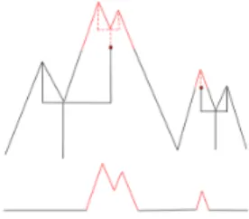
with each of its edges having unit length. We can then imagine a particle starting from the root, traveling along the edges of the tree at speed 1 and exploring the tree from left to right — see Fig1.1. The contour path of the tree is simply defined as the current distance of the exploration particle to the root — see Fig1.2.
In this paper, we show that the contour path of theh-trimming of a rooted plane tree (and more generally theh-trimming of rooted real trees) is given by theh-cut of the original contour path; where the h-cut is constructed from the two-sided Skorohod reflection of the original contour path – see (1.4).
Real rooted trees. As already discussed, every rooted plane tree can be en-coded by its contour path which is a function in C0+(R+) – the set of continuous non-negative functions on R+ with f(0) = 0 and compact support. Conversely,
it is now well established that any f ∈ C0+(R+) encodes a real rooted tree in the following natural way – see againLe Gall (2005) for more details. Define
∀s, t∈R+, df(s, t) =f(s) +f(t)−2 inf
[s∧t,s∨t]f,
and the equivalence relation∼onR+ as follows
s∼t⇐⇒df(s, t) = 0.
The equivalence relation∼defines a quotient space
Tf = R+/∼
referred to as the tree encoded byf. The functiondf induces a distance onTf, and
we keep the notationdf for this distance. It can be shown that the pair (Tf, df)
defines a real tree in the sense that the two following properties are satisfied. For everya, b∈ Tf:
(i) (Unique geodesics.) There is a unique isometric map ψa,b from
[0, df(a, b)] intoTf such thatψa,b(0) =aandψa,b(df(a, b)) =b.
(ii) (Loop free.) If q is a continuous injective map from [0,1] into Tf , such
thatq(0) =aand q(1) =b, we haveq([0,1]) =ψa,b([0, df(a, b)]).
In the following, for any x, y ∈ Tf, [x, y] will denote the geodesic from x to y,
i.e., [x, y] is the image of [0, df(x, y)] by ψx,y. We will denote bypf the canonical
projection fromR+toTf which can be thought of as the position of the exploration
particle at time t. In the following, ρf =pf(0) will be referred to as the root of
the tree Tf. In what follows, real trees will always be rooted, even if this is not
mentioned explicitly.
df induces a natural partial ordering on the rooted tree Tf : v0 v (v0 is an
ancestor ofv) iff
df(v, v0) = df(ρf, v)−df(ρf, v0).
We note that this partial ordering is directly related to the sub-excursions nested in the functionf. Indeed, for anys, t≥0,pf(t)pf(s) if and only if inf[t∧s,t∨s]f =
f(t), which is equivalent to saying that t is the ending time or starting time of a sub-excursion off starting from levelf(t) and straddling times– see Fig1.1and
1.2.
Finally, for anyx, y∈ Tf, the most recent common ancestor ofxandy– denoted
byx∧y– is defined as sup{z∈ Tf :zx, y}. From the definition of our genealogy,
for anyt1, t2∈R+, we must have
with the height of the most recent common ancestor being given by
f(s) = min
[t1∧t2,t1∨t2] f.
Figure 1.1. Exploration of a plane tree. The exploration particle
travels along each branch twice : first on the left and away from the root, and then on the right and towards the root. The root of the red sub-tree belongs to the2-trimming of the tree.
Figure 1.2. Contour path. The red portion of the curve is a sub-excursion of height 2 corresponding to the exploration of the red sub-tree on the left panel.
Trimming and the two-sided Skorohod reflection. As in Evans (2005), for every h >0, we define theh-trimming of the real tree (Tf, df) as the (possibly
empty) sub-tree
Trh(Tf) :={x∈ Tf : sup y∈Tf : yx
df(x, y)≥h}, (1.2)
which consists of all the points inTf having at least one leaf above them at distance
greater or equal toh. (Note that Trh(Tf) is not empty if and only if sup[0,∞)f ≥h.)
As already mentioned, one of the main results of this paper is the relation between the h-trimming of a real rooted tree and the two-sided Skorohod reflection of its contour path. The one-sided Skorohod reflection is well known among probabilists. Given a continuous function f starting from x ≥ 0, it is simply defined as the following transformation
Γ0(f)(t) := f(t) −(inf
[0,t]
The resulting path obviously remains non-negative and the function
c(t) := −(inf[0,t]f ∧0) is easily seen to be the unique solution of the so-called
(one-sided) Skorohod equation, i.e., c is the unique continuous function c on R+ such thatc(0) = 0 and
(1) Γ0(f)(t) :=f(t) +c(t) is non-negative. (2) cis non-decreasing.
(3) c does not vary off the set {t : Γ0(f)(t) = 0}, i.e., the support of the measuredcis contained in Γ0(f)−1({0}) .
See Lemma 6.17 in Karatzas and Shreve (1991) for a proof of this statement. Intuitively, the function c, which will be referred to as the compensator of the reflection in the rest of this paper, can be thought of as the minimal amount of upward push that one needs to exert on the pathf to keep it away from negative values. The Skorohod equation states that the reflected path is completely driven byf when it is away from the origin, while it is repealed from negative values by the compensator upon reaching level 0. The following theorem is a generalization of the Skorohod equation to the two-sided case. See also Fig. 1.3.
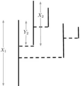
Figure 1.3. A path (plain line) and its two-sided reflection (dashed line) on the interval[0, h].
Theorem 1.1 (Two-Sided Skorohod Reflection). Let h ≥ 0 and let f be a continuous function with f(0) ∈ [0, h]. There exists a unique pair of continuous functions(c0(f), ch(f))with c0(f)(0) =ch(f)(0) = 0satisfying the three following
properties.
(1) Λ0,h(f)(t) := f(t) +ch(f)(t) +c0(f)(t)is valued in [0, h].
(2) c0(f)(resp., ch(f)) is a non-decreasing (resp., non-increasing) function.
(3) c0(f)(resp., ch(f)) does not vary off the setΛ0,h(f)−1({0})
(resp., Λ0,h(f)−1({h}))
As noted byKruk et al.(2007), existence and uniqueness to the Skorohod prob-lem follow directly from Lemma 2.1, 2.3 and 2.6 in Tanaka(1979). In the rest of this paper, Λ0,h(f) will be referred to as the two-sided Skorohod reflection of the
pathf on [0, h], while the pair of functions (c0(f), ch(f)) will be referred to as the
compensators associated with the functionf. In the same spirit as the one-sided reflection, the compensatorch(f) (resp., c0(f)) can be thought of as the minimal
amount of downward (resp., upward) push at levelh(resp., 0) that one has to exert onf to keep the path Λ0,h(f) inside the interval [0, h]. In other words, adding the
compensators c0(f) and ch(f) to f is the “laziest way” of keeping f inside the interval [0, h].
Letf be a continuous function onR+withf(0) = 0 (with no restriction on the
support and on the sign off). For such a function, define theh-cut of the function
f as
fh := f−Λ0,h(f) =−c0(f)−ch(f). (1.4)
fh is also characterized by the following interesting variational property.
Lemma 1.2. Let f be a non-negative continuous function on R+ with f(0) = 0. For everyT ≥0,fh is a solution of the following minimization problem:
Inf{TV(g,[0, T]) : g s.t. g(0) = 0, 0≤f−g≤h} (1.5)
whereT V(g,[0, T]) denotes the total variation ofg on the interval[0, T]
Proof: Let g := f −h/2 and (c−h/2(g), ch/2(g)) the compensators at −h/2 and
h/2 for the two-sided reflection reflection of g on [−h/2, h/2]. As an immediate corollary of Proposition 2 inMi lo´s(2013), we get that when f ≥0, the function
h/2−c−h/2(g)−ch/2(g), whereg:=f−h/2 is a minimizer of the following problem:
Inf{TV0(g,[0, T]) : g s.t. 0≤ ||f −g||∞,[0,T] ≤h/2}. (1.6)
(regardless of the value ofT) where|| · ||∞,[0,T] is the sup norm on [0, T].
The reflection of g =f −h/2 on the interval [−h/2, h/2] is obtained from the reflection off on the interval [0, h] by a translation of−h/2 which implies that
(c−h/2(g), ch/2(g)) = (c0(f), ch(f)).
Combining this with the result inMi lo´s(2013) stated above yields thath/2−c0(f)−
ch(f) is a minimizer of (1.6). Since the total variation is invariant under translation
by a constant, our result follows.
Informally, the previous result states that up to a linear transformation, fh is
the function of minimal total variation satisfying the constraint 0 ≤ f −g ≤ h.
1 Our main theorem states that the contour path of the h-trimming of a tree is
simply given by theh-cut of its original contour path.
Theorem 1.3. Let f ∈C0+(R+) and let us assume that the h-trimming of T
f is
not empty.
(1) The h-cut fh belongs toC0+(R+).
(2) Theh-trimming of the real tree(Tf, df)is identical to the real tree(Tfh, dfh)
(up to a root preserving isometry).
1For more information on the interesting minimization problem (1.5), we refer the reader to
To state our next result, we need to introduce some extra notations. For a continuous function f with f(0) = 0, definetn(f)≡tn (resp.,Tn(f)≡Tn) to be
thenthreturning time at level 0 (resp.,h) of Λ
0,h(f) andsn(f)≡sn to be thenth
exit time at 0 of Λ0,h(f) as follows. t0= 0, and forn≥1
Tn := inf{u > tn−1 : Λ0,h(f)(u) =h}
tn := inf{u > Tn : Λ0,h(f)(u) = 0}
sn := sup{u∈[tn−1, tn) : Λ0,h(f)(u) = 0} (1.7)
with the convention that sup{∅},inf{∅}=∞. See also Fig. 1.3. LetNh(f) be the
number of returns of Λ0,h(f) to 0, i.e.,
Nh(f) := sup{n: tn<∞}.
Finally, define{Xn(f)} ≡ {Xn}and{Yn(f)} ≡ {Yn},
∀n≥1, Xn(f) := fh(tn)−fh(sn),
Yn(f) := fh(tn−1)−fh(sn). (1.8)
As we shall see below (see Theorem1.5(2)), whenf is a Brownian excursion, the quantityXn(f) (resp.,Yn(f)) simply coincides with the amount of Brownian local
time accumulated by the reflected path Λ0,h(f) at h (resp., 0) on the interval
[tn−1, tn].
Proposition 1.4. Let f ∈C0+(R+) and let us assume that theh-trimming ofT
f
is not empty. Theh-trimming of Tf is equal (up to a root preserving isometry) to
the tree generated inductively according to the following algorithm – see Fig1.4.
(Step 1.) Start with a single branch of lengthX1(f).
(Step n,n≥2) If n=Nh(f)stop. Otherwise, let zn−1 be the tip of the (n−1)th branch. On the ancestral line[ρ, zn−1], graft a branch of lengthXn(f)at a distance
Yn(f)from the leafzn−1.
Figure 1.4. Schematic representation of the algorithm generating
theh-trimming of a tree from the two-sided reflection of its contour path.
Relation with standard binary trees. Recall that standard binary trees have branches (1) that have i.i.d. exponential life time with meanα, and (2) when
they die, they either give birth to two new branches, or have no offspring with equal probability 1/2. The algorithm described in Proposition 1.4 is reminiscent of a classical construction of standard binary trees (see e.g., Le Gall (1989)), for which (X1(f),{(Xn(f), Yn(f))}2≤n≤Nh(f)) is replaced with ( ˜X1,{( ˜Xn,Y˜n)}2≤n≤N˜)
where ˜X1,Y˜2,X˜2,Y˜3,· · · is an infinite sequence of independent exponential r.v.’s
with parameterαand the algorithm stops at step ˜N, with ˜ N := inf{n : n ∑ i=1 ( ˜Xi−Y˜i+1)<0}. (1.9)
(Note that this stopping condition is quite natural: the quantity∑ni=1( ˜Xi−Y˜i+1)
is the height of the nthintercalated branching point. We stop the algorithm once the branching point has negative height.) Using Proposition1.4, we easily recover a result due toNeveu and Pitman(1989), relating theh-trimming of the tree encoded by a Brownian excursione with standard binary trees (see item 1 in the following theorem). Further, the next theorem provides the joint distribution of the treeTe
and its trimmed version Trh(Te) (see item 2). In the following, for a path w, we
define lh(w)(t) := lim ε↓0 1 2ε|{s∈[0, t] : Λ0,h(w)(s)∈[h−ε, h]}| l0(w)(t) := lim ε↓0 1 2ε|{s∈[0, t] : Λ0,h(w)(s)∈[0, ε]}|, (1.10)
provided that those limits exist. lh(w) (resp.,l0(w)) will be referred to as the local
time of Λ0,h(w) ath(resp., at 0).
Theorem 1.5. Letebe a Brownian excursion conditioned on having a height larger thanh.
(1) Theh-trimming of the tree(Te, de)is a standard binary tree with parameter
α=h/2.
(2) For1≤i≤Nh(e),
• Xi(e) a.s. coincides with the local time of Λ0,h(e) at h accumulated
between[ti−1(e), ti(e)], i.e., Xi(e) =lh(e)(ti)−lh(e)(ti−1).
• Yi(e) a.s. coincides with the local time of Λ0,h(e) at 0 accumulated
between[ti−1(e), ti(e)].
The maximum of a sticky Brownian motion. Our final application of Theorem 1.3 relates to the sticky Brownian motion. Given a filtered probability space (Ω,G,{Gt}t≥0,P), a sticky Brownian motion, with parameter θ > 0, is
de-fined as the adapted process taking value on [0,∞) solving the following stochastic differential equation (SDE):
dzθ(t) = 1zθ(t)>0dw(t) + θ1zθ(t)=0dt, (1.11) where (w(t); t≥0) is a standard Gt-Brownian motion. Intuitively,zθis driven by
waway from level 0, and gets an upward push upon reaching this level, keeping the process away from negative values. Sticky Brownian motion were first investigated by Feller (1957) on strong Markov processes taking values in [0,∞) that behave like Brownian motion away from 0. We refer the reader to Varadhan(2001) for a good introduction on this object.
Ikeda and Watanabe showed that (1.11) admits a unique weak solution. The result was later straightened byChitashvili(1989) andWarren(1999) who showed that zθ is not measurable with respect to w and that, in order to construct the
processzθ, one needs to add some extra randomness to the driving Brownian motion
w. In Warren(2002), Warren did exhibit this extra randomness and showed that it can be expressed in terms of a certain marking procedure of the random tree induced by the one-sided Skorohod reflection of the driving Brownian motion w
(more on that in Section4).
Among the first applications related to sticky Brownian motions, we citeYamada
(1994) andHarrison and Lemoine (1981) who studied sticky random walks as the limit of storage processes. More recently,Sun and Swart (2008) introduced a new object called the Brownian net which can be thought of as an infinite family of one-dimensional coalescing-branching Brownian motions and in which sticky Brownian motions play an essential role (see alsoNewman et al.(2010)).
Building on the approach of Warren (2002), and using Theorem 1.3, we will show that the law of the maximum of a sticky Brownian motion can be expressed in terms of the local time of the two-sided reflection of its driving Brownian motion
won the interval [0, h].
In the following, λ0,h(·) will refer to the linear function reflected at 0 and h,
i.e., the function obtained by a linear interpolation of the points {(2n·h,0)}n∈Z
and {((2n+ 1)·h), h}n∈Z. For any continuous function f, thestandardreflection
of f on [0, h] (as opposed to the two-sided Skorohod reflection) will refer to the transformation λ0,h(f). In Warren (1999), the one-dimensional distribution of a
sticky Brownian motion conditionally on its driving process was given. The follow-ing theorem provides the one-dimensional distribution of the maximum of a sticky Brownian motion conditionally on its driving process.
Theorem 1.6. Let h >0 and let(zθ(t), w(t);t≥0)be a weak solution of equation (1.11) starting at(0,0). Λ0,h(w) is distributed as a Brownian motion reflected (in
the standard way) on[0, h]and we denote bylh(w)its local time ath(see (1.10)).
Then, P ( max [0,t] z θ ≤ h| σ(w) ) = exp(−2θ lh(w)(t)),
wherelh(w)is the local time athfor the pathΛ
0,h(w)(see (1.10)).
2. Proof of Theorem 1.3 and Proposition 1.4
In the following, a nested sub-excursion of the functionf ∈C0+(R+) will refer to any section of the pathf on an interval [t−, t+] such that∀t∈[t−, t+],inf[t−,t]f =
f(t−) = f(t+) – see Fig 1.2. The height of such a sub-excursion is defined as
max[t−,t+]f−f(t+).
Letpf(t) be the canonical projection from R+ to Tf, which can be thought of
as the position of the exploration particle at timet. By definition,pf(t) belongs to
Trh(Tf) if and only if there existsssuch that inf[t∧s,t∨s]f =f(t) andf(s)−f(t)≥h,
which is equivalent to saying that t is the ending time or starting time of a sub-excursion (nested inf) of height at leasthstarting from levelf(t). We claim that the extreme points of Trh(Tf) – orleaves– are contained in the set of points of the
In order to see that, lettbe the time extremity of a sub-excursion of height strictly larger thanh. By continuity, this sub-excursion must contain another sub-excursion of height greater or equal toh. Thus,pf(t) must have at least one descendant and
can not be a leaf. As claimed earlier, this shows that the leaves must be visited at the time extremities of some sub-excursion of heightexactlyh. 2
Let us now define inductively {τn(f)}n≥0 ≡ {τn}n≥0, {θn(f)}n≥1 ≡ {θn}n≥1
and{σn(f)}n≥0≡ {σn}n≥0 as follows : τ0= 0, σ0= 0 and
θn+1 = inf{s > τn: f(s)−h= inf [τn,s] f}. τn+1 = inf{s > θn+1: sup [θn+1,s] f =f(t) +h}, σn+1 = sup{s∈[τn, τn+1] :f(s) = inf [τn,s] f}. (2.1)
with the convention that inf{∅},sup{∅}=∞. See also Fig. 1.3.
As already noted inNeveu and Pitman(1989) (although under a slightly different form), the sequences{τn}{n: τn<∞}and{σn}{n :σn<∞} play a key role in the tree Trh(Tf), being respectively related to the exploration times for the leaves and the
branching points respectively.
First, the reader can easily convince herself that the set of finite τn’s coincide
with the completion times of all the sub-excursions nested in the functionf which are exactly of heighth(seeNeveu and Pitman(1989) for more details). As already discussed, this implies that{pf(τn)}{n:τn<∞} contains the set of leaves of the tree Trh(Tf).
Secondly, the very definition of theσi’s implies that for everym < n, inf[τm,τn]f=
f(σk) for somek∈ {m+ 1,· · ·, n}. From (1.1), this implies thatpf(τn)∧pf(τm) –
the most recent common ancestor ofpf(τn) andpf(τm) – is given by somepf(σk).
We now show that the timesσn(f) andτn(f) also appear quite naturally in the
two-sided Skorohod reflection. Recall from the introduction, that tn (resp., sn)
refers to thenth returning time (exit time) of Λ0,h(f) at level 0 (see (1.7)).
Proposition 2.1. For every continuous function f with f(0) = 0 and for every
n≥1,
(1) τn(f) is thenth returning time to level 0 ofΛ0,h(f), i.e.,τn(f) =tn(f).
(2) σn(f) is thenth exit time at level 0 of Λ0,h(f), i.e.,σn(f) =sn(f).
(3) The function fh = f −Λ0,h(f) is non-decreasing (resp., non-increasing)
on [σn+1(f), τn+1(f)] (resp., on[τn(f), σn+1(f)]). In particular, {fh(σi)}
(resp.,{fh(τi)}) coincide with the local minima (resp., local maxima) offh.
See also Fig. 1.3 for a pictorial representation of the next proposition. As we shall see, this proposition is a consequence of elementary results on the two-sided Skorohod reflection that we now expose. We start by introducing some notations:
∀f, ∀t >0, RT(f)(t) := 1t≥T(f(t)−f(T)).
In other words,RT(f) is constant on [0, T] and follows the variation off afterwards.
The next elementary lemma states that the reflection of a path can be obtained
2Note that we only have an inclusion. For example, lettbe the starting time of a sub-excursion
of height exactlyh, and lettebe the ending time of this excursion. Ifteis also the starting time
by successively reflecting the path up to someT and then reflecting the remaining portion of the path fromT to∞.
Lemma 2.2. For any continuous function f withf(0)∈[0, h]andT ≥0,
∀t < T, Λ0,h(f)(t) = Λ0,h(f(· ∧T)) (t), ∀t≥T, Λ0,h(f)(t) = Λ0,h ( RT(f) + Λ0,h(f)(T) ) (t).
Proof: In the following, we write
LT(f)(t) := RT(f)(t) + Λ0,h(f)(T),
and for any continuous functionF withF(0)∈[0, h], we denote by (c0(F), ch(F))
the pair of compensators solving the Skorohod equation for the two-sided reflection ofF on the interval [0, h]. Fory= 0, h, define
∀t≥0, ˜cy(t) := cy(f(· ∧T))(t) + cy(LT(f))(t).
We will show that (˜c0,˜ch) solves the two-sided Skorohod equation for f. We first
need to prove that the functionG(t) :=f(t) + ˜ch(t) + ˜c0(t) is valued in [0, h]. First
G(t) = f(t∧T) + ∑ y=0,h cy(f(· ∧T))(t) + LT(f)(t) + ∑ y=0,h cy(LT(f))(t) −Λ0,h(f)(T) = Λ0,h(f(· ∧T))(t) + Λ0,h◦LT(f)(t) −Λ0,h(f)(T) = Λ0,h(f)(t∧T) + Λ0,h◦LT(f)(t)−Λ0,h(f)(T)
where the first equality follows from the factf(t) =f(t∧T)+LT(f)(t)−Λ0,h(f)(T)
and the last equality only states that the reflection of the function f(· ∧T) (the functionf “stopped” atT) is the reflection off stopped atT (this can directly be checked from the definition of the two-sided Skorohod reflection).
The function LT(f) is constant and equal to Λ
0,h(f)(T) on the interval [0, T].
This easily implies that its reflection is also identically Λ0,h(f)(T) on the same
interval. Thus, the latter equality implies that
G(t) := {
Λ0,h(f)(t) ift < T ,
Λ0,h◦LT(f)(t) otherwise.
(2.2) (2.2) implies thatG(t) belongs to [0, h], hence proving that the first requirement of the Skorohod equation (see Theorem1.1) is satisfied. The second requirement – the function ˜ch (resp., ˜c0) non-increasing (resp., non-decreasing) – is obviously
satisfied since the function ˜ch (resp., ˜c0) is constructed out of a compensator ath
(resp., at 0). Finally, fory= 0, h, we need to show that the support of the measure
d˜cy is included in the set G−1({y}). In order to see that, we use the fact that the support of dcy(LT(f)) and dcy(f(· ∧T)) are respectively included in [T,∞] and [0, T] — using the fact that if a function g is constant on some interval, its compensator does not vary on this interval. As a consequence, fory= 0, h
Supp(˜cy)∩[0, T] = Supp(cy(f(· ∧T)))∩[0, T]
where Supp denotes the support of the measure under consideration. Further, Supp(cy(f(· ∧T)) ⊂ {t : Λ
0,h(f(· ∧T))(t) = y}. Since Λ0,h(f(· ∧T)) and G
coincides on [0, T] (by (2.2)), we get that on [0, T] the compensator ˜cyt only varies onG−1({y}). By an analogous argument, one can show that the same holds on the
interval [T,∞]. Hence, the third and final requirement of the Skorohod equation holds for ˜cy, y = 0, h. This shows that (˜c0,c˜h) solves the two-sided Skorohod
reflection. Combining this with (2.2) ends the proof of our lemma.
Let h ≥ 0. For any continuous function f with f(0) ≤ h, let us define the one-sided reflection (with downward push) ath– denoted by Γh(f) – as
Γh(f) :=f−(sup
[0,t]
f−h)∨0.
Along the same lines as the one-sided reflection at 0 (as introduced in (1.3)), the functionc(t) =−(sup[0,t]f −h)∨0 can be interpreted as the minimal amount of downward push necessary to keep the path f below level h. More precisely, this function is easily seen to be the only continuous functioncwithc(0) = 0 satisfying the following requirements: (1) f +c ≤h, (2) c is non-increasing and, (3) c does not vary off the set{t≥0 : f(t) +c(t) =h}.
Lemma 2.3. For everyT ≥0 and every continuous functionF with F(0)∈[0, h]
such that Γh(F)≥0 (resp.,Γ0(F)≤h) on[0, T], we must have
∀t∈[0, T], Λ0,h(F)(t) = Γh(F)(t) (resp.,Λ0,h(F)(t) = Γ0(F)(t)).
Proof: Let us consider a continuousF withF(0)∈[0, h] and such that Γh(F)≥0
on [0, T]. Let us prove that Λ0,h(F) = Γh(F) on [0, T]. We aim at showing that
(0,−(sup[0,t]F −h)+) coincides with the pair of compensators of F on the time
interval [0, T]. First,
Γh(F) = F + 0 + (−(sup
[0,t]
F−h)∨0)
belongs to [0, h] since Γh(F)≤hand under the conditions of our lemma Γh(F)≥0.
Secondly, using the fact that −(sup[0,t]F−h)∨0 is the compensator for the one-sided case (ath), this function is non-increasing and only decreases when Γh(F) is at level h. This shows that Γh(F) coincides with the two sided reflection of f on the interval [0, h]. The case Γ0(F)≤hcan be handled similarly.
Proof of Proposition2.1: In order to prove Proposition2.1, we will now proceed by induction onn.
Step 1. We first claim that σ1 ≤ θ1. When θ1 = ∞, this is obvious. Let us
assume that θ1<∞and let us assume that σ1 > θ1. The definition ofθ1 implies
that Γ0(f)(θ
1) = hand thus θ1 belongs to an excursion of Γ0(f) away from 0 (of
height at leasth), whose time interval we denote by [t−, t+]. Sinceσ1 was defined
as the last visit at 0 of Γ0(f) before time τ
1 (see (2.1)) andσ1 is assumed to be
greater thanθ1,σ1≥t+ and the excursion of Γ0(f) on [t−, t+] must be completed
beforeτ1. On the other hand,
h = ( f(θ1)− inf [0,θ1] f ) − ( f(t+)− inf [0,t+] f ) = f(θ1)−f(t+) ≤ sup [θ1,t+] f −f(t+),
where we used the fact that inf[0,t]f must remain constant during an excursion
of Γ0(f) away from 0 in the second equality. By continuity of f, there must exist
s∈[θ1, t+] such that sup[θ1,s]f−f(s) =h, which implies thatτ1≤t+, thus yielding
a contradiction and proving thatσ1≤θ1.
Next, the strategy for proving the first step of our proposition consists in breaking the intervals [0, τ1] into three pieces: [0, σ1], [σ1, θ1] and [θ1, τ1]. In the following,
we assume thatτ1<∞. The complementary case is obvious.
First, on [0, σ1], we must have Γ0(f)< h sinceσ1 < θ1, and θ1 was defined as
the first time Γ0(f)(t) =h. By Lemma2.3, this implies that
∀t∈[0, σ1], Λ0,h(f)(t) = Γ0(f)(t) =f−inf
[0,t]
f, and Λ0,h(f)(σ1) = 0, (2.3)
where the latter equality follows directly from the definition ofσ1. Next by Lemma
2.2, we must have
∀t∈[σ1,∞], Λ0,h(f)(t) = Λ0,h(1·≥σ1(f −f(σ1))(t).
Using the fact that inf[0,t]f remains constant during an excursion of Γ0(f) away
from 0 and the fact thatf−inf[0,·]f < hon [0, θ1], it is easy to see thatθ1coincides
with the first visit of 1·≥σ1(f(·)−f(σ1)) ath. Further, sinceσ1is thelastvisit at
0 of Γ0(f) beforeτ
1, we must have
∀t∈(σ1, τ1), f(t)−inf [0,t]
f =f(t)−f(σ1)>0.
In particular, f −f(σ1)∈(0, h] on the interval (σ1, θ1] and thus, (0,0) solves the
Skorohod equation for 1·≥σ1(f−f(σ1)) on this interval. This yields
∀t∈(σ1, θ1), Λ0,h(f)(t) =f(t)−f(σ1)>0. (2.4)
Finally, we look at Λ0,h(f) on [θ1, τ1]. Using Λ0,h(f)(θ1) =h, Lemma 2.2implies
that
∀t∈[θ1, τ1], Λ0,h(f)(t) = Λ0,h(h+ 1·≥θ1(f(·)−f(θ1)).
A straightforward computation yields
∀t≤τ1, Γh(h+ 1·≥θ1(f(·)−f(θ1)) (t) = h+ 1t≥θ1(f(t)−sup
[θ1,t] f) By definition ofτ1, the RHS of the equality must remain positive on [θ1, τ1). Using
Lemma2.3, we get that
∀t∈[θ1, τ1), Λ0,h(f)(t) = Γh(f)(t) =f(t) +h−sup
[θ1,t] f >0,
and Λ0,h(f)(τ1) = 0 (2.5)
where the second equality follows from the very definition ofτ1. Finally, combining
(2.3)–(2.5) yields that Λ0,h(f) is continuous on [0, τ1], and further that
∀t∈[0, τ1], Λ0,h(f)(t) = f − ( 1t∈[0,σ1)·inf [0,t] f + 1t∈[σ1,θ1)·f(σ1) + 1t∈[θ1,τ1]·( sup [θ1,t] f −h) ) .
As a consequence, fh =f −Λ0,h(f) is non-increasing (resp., non-decreasing) on
σ1) is the first returning time (resp., exit time) at level 0. Indeed, piecing together
the previous results, we proved
Λ0,h(f)(t)< h, on [0, σ1) and Λ0,h(f)(σ1) = 0
Λ0,h(f)>0 on (σ1, τ1), and Λ0,h(f)(θ1) =h, Λ0,h(f)(τ1) = 0.
Step n+1. Let us assume Proposition 2.1 is valid up to rank n. Recall that
Rτn(f) = 1
t≥τn(f(t)−f(τn)). By Lemma2.2,
∀t∈[τn,∞), Λ0,h(f) = Λ0,h(Rτn(f)),
where we used the induction hypothesis to write Λ0,h(f)(τn) = 0. On the other
hand, it is straightforward to check from the definitions ofτn+1, θn+1 and σn+1 in
(2.1) that
σn+1(f) = σ1(Rτn(f)), τn+1(f) = τ1(Rτn(f)), θn+1(f) =θ1(Rτn(f))
Applying the case n = 1 to the function Rτn(f) immediately implies that our proposition is valid at stepn+ 1.
In order to prove Theorem1.3, we will combine Proposition2.1with the following lemma.
Lemma 2.4. Let (T1, d1) and (T2, d2) be two rooted real trees with only finitely many leaves. Fork= 1,2, let Sk = (zk1,· · · , zNk)∈ Tk such that the two following
conditions hold.
(1) Fork= 1,2,Sk contains the leaves of Tk.
(2) ∀i≤N, d1(ρ1, zi1) =d2(ρ2, z2i)and∀i, j≤N, d1(ρ1, z1i ∧z 1 j) =d2(ρ2, z2i ∧z 2 j),
whereρk is the root ofTk.
Under those conditions, there exists a root preserving isometry from T1 ontoT2. Proof: For k= 1,2 andm≤N, let Imk := [ρk, zmk]. Using the second assumption
of our lemma, the two ancestral linesIm1 andIm2 must have the same length. From
there, it easy to construct a root preserving isometry from Im1 ontoIm2 as follows.
SinceTk is a tree, there exists a unique isometric mapψkmfrom [0, dk(ρk, zmk)] onto
Ik
m, such thatψkm(0) =ρk andψmk(dk(ρk, zmk)) =zkm. Define
∀a∈Im1, φm(a) := ψm2 ◦(ψ
1
m)−
1(a).
Since d1(ρ1, zm1) = d2(ρ2, zm2), it is straightforward to show that φm defines an
isometry fromI1
montoIm2. Furthermore,φmpreserves the root,φm(zm1) =zm2 and
it is order preserving, i.e.,∀ab∈I1
m, φm(a)φm(b).
Next, we claim that if a ∈ I1
m∩Il1, then φm(a) = φl(a). We first show the
property for a = z1
m∧zl1. Using the isometry of φm and the root preserving
property, we have d2(ρ2, φm(zl1∧z 1 m)) = d1(ρ1, zl1∧z 1 m) = d2(ρ2, zl2∧z 2 m),
where the second equality follows from the second assumption of our lemma. Since
φm(a)∈Im2, it follows thatφm(z1l ∧z1m) =zl2∧zm2 – on the segmentIm2, a point is
that φl(zl1∧zm1) =zl2∧zm2. Let us now take any point a∈ Im1 ∩Il1. Under this
assumption, we must haveaz1
m∧zl1. Using the isometry property, this implies
d2(ρ2, φm(a)) = d2(ρ2, φl(a))
and using the order preserving property
φl(a), φm(a)zm2 ∧zl2,
since we showed thatφm(z1m∧z1l), φl(z1m∧z1l) =z2m∧z2l. It follows thatφm(a) =
φl(a), as claimed earlier.
We are now ready to construct the isometry fromT1 ontoT2. First, fork= 1,2,
any pointak ∈ Tk must belong to some ancestral line of the form [ρk, l], for some
leafl in the treeTk. By what we just proved, and sinceS1 contains all the leaves
ofT1, we can define a mapφfromT1into T2as follows
∀a∈ T1, φ(a) := φm(a) if a∈Im1.
SinceS2 contains all the leaves ofT2, and any ancestral line of the form [ρ1, zm1] is
mapped onto [ρ2, z2
m], the mapφis onto.
It remains to show that φ is isometric. Let a, b ∈ T1 and let us distinguish
between two cases. First, let us assume thataandb belong to the same ancestral line I1
m for some m ≤ N. Under this assumption, the property simply follows
from the isometry of φm. Let us now consider the case where a and b belong
to two distinct ancestral lines: a ∈ Im1 but a /∈ Il1, and b ∈ Il1 but b /∈ Im1; in such a way that a∧b = zl1∧z1m. Using the fact that both φm and φl are
isometric and order preserving, and φ(zl1∧zm1) =zl2∧z
2
m,φl(a)∈Il2, φm(a)∈Im2
we get that φ(a)∧φ(b) = z2
l ∧z
2
m. We can then write [φ(a), φ(b)] as the union
[z2 l ∧z 2 m, φ(a)]∪[zl2∧z 2 m, φ(b)] and write d2(φ(a), φ(b)) = d2(zl2∧z 2 m, φ(a)) +d2(zl2∧z 2 m, φ(b)) = d1(zl1∧z 1 m, a) +d1(zl1∧z 1 m, b) = d1(a, b)
where the second equality follows by applying the previous case to the pairs of points (z1l ∧z1m, a) and (zl1∧z
1
m, b).
In the following, we make the assumption that theh-trimming of the treeTf is
non-empty, i.e., that sup[0,∞)f ≥h.
Proof of Theorem 1.3: Recall thatC0+(R+) denotes the set of continuous non-neg-ative functions withf(0) = 0 and compact support. We start by showing the first item of our theorem, i.e., that f ∈ C0+(R+) implies that fh ∈ C0+(R
+). First, as
an easy corollary of Proposition 2.1, we get that for every continuous f ≥ 0, the functionfh =f −Λ0,h(f) is non-negative. This simply follows from the fact that
the local minima offh are attained on the set{σi}, on whichf(σi) =fh(σi) since
Λ0,h(f)(σi) = 0. Sincef(σi) ≥ 0, the function fh is non-negative. Secondly, we
show thatf ≥0 implies that Supp(fh)⊂Supp(f). In order to see that, lettbe such
that f(t) = 0. We have fh(t) =−Λ0,h(f)(t) and sincefh ≥0 and −Λ0,h(f)≤0,
it follows that fh(t) = 0 (and Λ0,h(f)(t) = 03). As a consequence, iff ∈C0+(R+)
thenfh∈C0+(R +).
3This also shows that Supp(Λ
Next, let us show that fh is such that the real tree (Tfh, dfh) is isometric to the h-trimming of the tree (Tf, df). is the contour function of the h-trimming of
the tree Tf (up to a root preserving isometry). For k ≤ Nh(f), Proposition 2.1
immediately implies that the maximum offh on [σk, σk+1) is attained at time τk
and that the set
Ik:={t∈[σk, σk+1) : fh(t) =fh(τk)}
is a closed interval. On the one hand, any timet∈[σk, σk+1) outside of this interval
is the starting or ending time of a sub-excursion with (strictly) positive height, and for such t, pfh(t) can not be a leaf. On the other hand, we havepfh(t) =pfh(t0) for t, t0 ∈ Ik. This implies that the only possible leaf of Tfh visited during the time interval [σk, σk+1) is given bypfh(τk) and thus, that the set of leaves ofTfh is included in the finite set of points{pfh(τn)}{n: τn<∞}.
As explained at the beginning of this section, any leaf of the tree Trh(Tf) must
be explored at some finite τn, i.e., the set of leaves of Trh(Tf) is a subset of
{pf(τn)}{n:τn<∞}.
In order to prove our result, we use Lemma2.4withzi1=pf(τi) andz2i =pfh(τi) and
N=Nh(f) =|{n : τn(f)<∞}|.
First, item 1 of Proposition 2.1implies that the height of the vertices pf(τi) and
pfh(τi) are identical, i.e., that f(τi) = fh(τi) since Λ0,h(f)(τi) = 0. In order to show that Trh(Tf) andTfh are identical (up to a root preserving isomorphism), it is sufficient to check that
∀i < j, inf
[τi,τj]
f = inf
[τi,τj]
fh,
i.e., that the height of the most recent common ancestor of the vertices visited at
τiandτj is the same in both trees. To justify the latter relation, we first note that
the definition of the σm’s (see (2.1)) implies that inf[τi,τj]f must be attained at some σk (for some k∈ {i+ 1,· · ·, j}). On the other hand, the third item of the
Proposition2.1implies that the same must hold forfhsince the set of local minima
offhcoincide with{fh(σi)}. Since f(σi) =fh(σi),(si =σi by the second item of
Proposition2.1 and Λ0,h(f)(si) = 0), Theorem1.3follows.
Proof of Proposition1.4: Let us define
Tn
fh := {z∈ Tfh : ∃t≤tn, pfh(t) =z},
the set of vertices in Tfh visited up to time tn. Tfh can be constructed recursively by adding toTn
fh all the vertices inT
n+1
fh \ T
n
fh for everyn < N, whereN ≡Nh(f). (Indeed, by definition of a real tree from its contour path, if a point is visited at a given time, its ancestral line must have been explored before that time. Thus, if all the leaves have been explored at a given time – e.g., attN–vertex has been visited
at least once before that.) For everyn < N, let us show that the setTfn+1 h \ T
n fh is a branch (more precisely, a segment [a, b]\ {a} witha, b∈ Tfh and ab)
(i) with tipb=pfh(tn+1) – i.e., ∀z∈ T
n+1
fh \ T
n
fh, zpfh(tn+1) – (ii) attached toa=pfh(sn+1) – i.e., ∀z∈ T
n+1
fh \ T
n
fh, pfh(sn+1)z. (iii) pf(sn+1) belongs to the ancestral line [ρfh, pfh(tn)].
Letn < N and lett∈(tn, tn+1]. The definition of the real treeTfh implies that the pointpfh(t) has been visited before tn if and only if there existss≤tn such that
inf
[s,t]fh=fh(t) =fh(s), (2.6)
i.e.,t must be the ending time of a sub-excursion straddlingtn. On the one hand,
sincefh is non-increasing on [tn, sn+1] (by Proposition2.1), we have
∀t∈[tn, sn+1], inf [tn,t]
fh=fh(t). (2.7)
Sincefh(0) = 0 andfh(t)≥0, one can finds≤tn such that (2.6) is satisfied (using
the continuity offh). Thus, every point visited on the time interval [tn, sn+1] has
already been visited beforetn and does not belong to Tfnh+1\ T
n fh.
On the other hand, the functionfh is non-decreasing on [sn+1, tn+1] (again by
Proposition2.1). Let us define ¯
θn+1= sup{t∈[sn+1, tn+1] : fh(t) =fh(sn+1)}
(with the convention sup{∅} = tn+1). First, the definition of our real tree Tfh implies that any pfh(t) with t ∈ [sn+1,θ¯n+1] coincides with pfh(sn+1). Secondly, for anyt∈[¯θn+1, tn+1], and anys≤tn
inf
[s,t]fh≤fh(sn+1)< fh(t)
which implies that any point visited during the interval (¯θn+1, tn+1] belongs to
Tn+1
fh \ T
n
fh. Furthermore, the previous inequality implies that
∀t∈(¯θn+1, tn+1], pfh(t)pfh(sn+1). (2.8) Finally,
∀t∈[¯θn+1, tn+1], inf [t,tn+1]
fh=fh(t),
which implies that
∀t∈[¯θn+1, tn+1], pfh(t)pfh(tn+1). (2.9) Combining the results above, we showed the claims (i)–(iii) made earlier: Tfn+1
h \T
n fh is a branch with tippf(tn+1) (see (2.9)) attached at the pointpfh(sn+1) (see (2.8)), which belongs to [ρfh, pfh(tn)] (see (2.7) applied tot =sn+1). The length of the branch is given by
fh(tn+1)−fh(sn+1) =Xn+1(f), (2.10)
(height of the (n+ 1)thleaf−height of the attachment point) and the distance of
the attachment point from the leafpfh(tn) is given by
fh(tn)−fh(sn+1) =Yn+1(f). (2.11)
(Height of thenthleaf−height of the attachment point.) This completes the proof
3. Proof of Theorem 1.5
Next, letebe a Brownian excursion conditioned on having a height greater than
hand let{(Xn(e), Yn(e))}i≤Nh(e) be defined as in (1.8), i.e.,
∀n≥1, Xn(e) = eh(tn)−eh(sn)
Yn(e) = eh(tn−1)−eh(sn),
with tn ≡tn(e), sn ≡sn(e) and letNh(e) be the number of returns of Λ0,h(e) at
level 0. As discussed in the introduction (see the discussion preceding Theorem
1.5), in order to prove that the trimmed tree Trh(Te) is a binary tree, we need
to show that (X1(e),{(Xi(e), Yi(e))}2≤i≤Nh(e)) is identical in law with a sequence ( ˜X1,{( ˜Xi,Y˜i)}2≤i≤N˜), where ˜X1,Y˜2,X˜2,· · · is an infinite sequence of independent
exponential random variables with meanh/2 and ˜ N := inf{n : n ∑ i=1 ( ˜Xi−Y˜i+1)<0}.
The idea of the proof consists in constructing a coupling between (X1(e),{(Xi(e), Yi(e))}2≤i≤Nh(e)) and ( ˜X1,
˜
Y2,X˜2,· · ·) as follows. Letwbe a
Brow-nian motion withw(0) = 0, independent of the excursione, and define ˜
w(t) := e(t) +w((t−K(e))∨0) whereK(e) := sup{t >0 : e(t)>0}, (3.1) obtained by pasting the processwat the end of the excursione. Finally, forn≥1, define ˜Xn:=Xn( ˜w) and ˜Yn:=Yn( ˜w).
First, the support of Λ0,h(e) is included in the support ofe. (This was established
in the course of the proof of Theorem1.3.) As a consequence, for everyn≤Nh(e),
we must have tn(e), sn(e) ≤ K(e) (recall that for n ≤ Nh(e), tn(e) and sn(e)
coincide with thenthfinitereturning and exit times at 0). Sinceeand ˜w(and their reflections) coincide up to K(e), this implies that sn(e) = sn( ˜w), tn(e) = tn( ˜w)
and that Xn(e) = ˜Xn, Yn(e) = ˜Yn for n ≤ Nh(e). Theorem 1.5 is then a direct
consequence of our coupling and the two following lemmas.
Lemma 3.1. (1) ˜X1,Y˜2,X˜2,Y˜3,· · · is an i.i.d. sequence of independent expo-nential variables with parameter h/2. Further,Y˜1= 0.
(2) Fori≥1, • X˜i = lh( ˜w)(˜t i)−lh( ˜w)(˜ti−1), • Y˜i = l0( ˜w)(˜t i)−l0( ˜w)(˜ti−1), where˜ti:=ti( ˜w).
Lemma 3.2. Under our coupling,
Nh(e) = inf{n: n
∑
i=1
( ˜Xi−Y˜i+1)<0} a.s..
Proof of Lemma 3.1: Let us first prove that ˜Y1 = 0 and that ˜Y1 = l0( ˜w)(˜t1)−
l0( ˜w)(˜t0). Let
¯
T1:= inf{t: ˜w(t) =e(t) =h}.
Sinceeis a Brownian excursion with height larger thanh, ¯T1<∞and ˜w∈(0, h]
on (0,T¯1]. From there, it immediately follows that Λ0,h( ˜w) = ˜won [0,T¯1] and that
¯
(see (1.7) for a definition of T1( ˜w)). Further, ˜s1– the first exit time of Λ0,h( ˜w) at
level 0 – is equal to 0. Since ˜
Y1 = −(c0+ch)( ˜w)(0) + (c0+ch)( ˜w)(˜s1),
this implies ˜Y1 = 0. Finally, we also get that l0( ˜w)(˜t1)−l0( ˜w)(˜t0) = 0, since ˜t1
coincides with the first returning time of the reflected process at 0, and this process never hits 0 on the interval (0,˜t1).
Before proceeding with the rest of the proof, we start with a preliminary discus-sion. Let w0 be a one-dimensional Brownian motion starting at x∈[0, h]. Recall that the one-sided Skorohod reflection Γ0(w0) is distributed as the absolute value
of a standard Brownian motion, and the compensatorc(w0)(t) =−(inf[0,t]w∧0) is
the local time at 0 of Γ0(w0). A proof of this statement can be found inKaratzas
and Shreve(1991). By following the exact same steps, one can prove an analogous statement for the two-sided case, i.e., that for any Brownian motionw0 starting at some x∈[0, h], Λ0,h(w0) is identical in law with λ0,h(w0) (the standard reflection
of the Brownian motionw0 – see Section1in the discussion preceding Theorem1.6
for a description ofλ0,h(w0)) and that−ch(w0) andc0(w0) are respectively the local
times athand 0 of this process.
Next, let us define ˜tn =tn( ˜w) and ˜sn =sn( ˜w) and recall that the h-cut ˜wh is
defined as ˜ wh= ˜w−Λ0,h( ˜w) =−c0( ˜w)−ch( ˜w). By definition of ˜Xn, we have ˜ Xn = w˜h(˜tn)−w˜h(˜sn) = ch( ˜w)(˜sn)−ch( ˜w)(˜tn) = ch( ˜w)(˜tn−1)−ch( ˜w)(˜tn). (3.2)
The second line follows from the fact that c0( ˜w) does not vary off the set Λ0,h( ˜w)−1({0}) and Λ0,h( ˜w) > 0 on (˜sn,˜tn); the third line is a consequence of
the fact thatch( ˜w) does not vary off the set Λ
0,h( ˜w)−1({h}) and Λ0,h( ˜w)< h on
(˜tn−1,s˜n). By an analogous argument, one can prove that
˜
Yn = c0( ˜w)(˜tn)−c0( ˜w)(˜tn−1). (3.3)
With those results at hand, we are now ready to prove our lemma. In the first paragraph, we already argued that Λ0,h( ˜w) = ˜won [0,T¯1]. By Lemma2.2,
∀t≥0, r(t) := Λ0,h( ˜w)(t+ ¯T1)
= Λ0,h( ˜w(·+ ¯T1))(t).
By William’s decomposition of a Brownian excursion conditioned on having a height larger than 1, the process ˜w(·+ ¯T1) is distributed as a standard Brownian motion
starting at level 1. Hence, the discussion above implies that the pathris identical in law with a reflected Brownian motion (where the reflection is a two-sided “stan-dard reflection”) starting at levelh. Further, the compensatorsc0( ˜w)( ¯T
1+·) and
−ch( ˜w)( ¯T
1+·) are the local times at 0 and hfor the process r. Using (3.2)–(3.3),
we easily obtain that ˜Xn (resp., ˜Yn) is the local time accumulated ath(resp., 0),
forn≥1 (resp.,n≥2) on [˜tn−1,t˜n]. This completes the proof of the second part of
our lemma. Finally, by standard excursion theory, ˜X1,Y˜2,X˜2,Y˜3,· · · are i.i.d.
ex-ponential random variables with meanh/2. (Independence follows from the strong Markov property, whereas ˜Xi and ˜Yi+1are distributed as the amount of Brownian
local time accumulated at 0 before occurrence of an excursion of height larger or equal toh.)
Proof of Lemma 3.2: Recall that ˜
Xn= ˜wh(˜tn)−w˜h(˜sn) and ˜Yn= ˜wh(˜tn−1)−w˜h(˜sn),
where we wrote ˜tn=tn( ˜w), ˜sk=sk( ˜w). Thus,
˜ wh(˜sn+1) = [ n ∑ i=1 ( ˜wh(˜ti)−w˜h(˜ti−1))] − ( ˜wh(˜tn)−w˜h(˜sn+1)) = [(−Y˜1+ ˜X1) + (−Y˜2+ ˜X2) +· · ·+ (−Y˜n+ ˜Xn)] −Y˜n+1 = −Y˜1+ n ∑ i=1 ( ˜Xi−Y˜i+1) = n ∑ i=1 ( ˜Xi−Y˜i+1),
where the last equality follows from the fact that ˜Y1= 0 (see item 1 of the previous
lemma).
Let us now show thatNh(e) = inf{n:
∑n
i=1( ˜Xi−Y˜i+1)<0}a.s.. First, let us
take n < Nh(e). On the one hand, we already argued that ˜sn+1 ≤K(e). On the
other hand, ˜wh≥0 on [0, K(e)] sinceeh≥0 (by Theorem1.3) and thatehand ˜wh
coincide up toK(e). Thus, ˜ wh(˜sn+1) = n ∑ i=1 ( ˜Xi−Y˜i+1)≥0.
Conversely, let us taken=Nh(e). By Proposition 2.1, ˜wh attains a minimum at
˜
sN˜
h(e)+1 on the interval [˜tNh(e),˜tNh(e)+1]. SinceK(e) ∈ [˜tNh(e),t˜Nh(e)+1], we get that 0 = ˜wh(K(e)) ≥ w˜h(˜sNh(e)+1) = N∑h(e) i=1 ( ˜Xi−Y˜i+1).
Since ˜Xi and ˜Yi are exponential random variables, this inequality is strict almost
surely. This completes the proof of the lemma. 4. Proof of Theorem 1.6
Let (zθ, w) be a weak solution of (1.11). Our proof builds on the approach of
Warren(2002). In this work, it is proved that the pair (zθ, w) can be constructed by adding some extra noise to the reflected process
ξ(t) :=w(t)−inf
[0,t]
w
as follows. First, there exists a uniqueσ-finite measure – here denoted by Lξ and
referred to as the branch length measure – on the metric space (Tξ, dξ) such that

![Figure 1.3. A path (plain line) and its two-sided reflection (dashed line) on the interval [0, h].](https://thumb-us.123doks.com/thumbv2/123dok_us/1422118.2690333/4.918.225.700.538.697/figure-path-plain-line-sided-reflection-dashed-interval.webp)