Orbital Dynamics in 3 He-A *l

(1)

772

Progress of Theoretical Physics, Vol. 63, No. 3, March 1980

Orbital Dynamics in

3

_He-A

_*l --I-Iomogencous Case--Haruo TAKAGI and Kazumasa MIYAKE

Department of Physics, Nagoya University, Nagoya 46 4 (Received November 15, 1979)

The orbital dynamics of the homogeneous superfluid 'He-A is investigated through micro-scopic calculation of the response function for the l-vector of the Cooper pairs. It is shown that Leggett and Takagi's phenomenological theory is justified in the region J (T)r:;}> 1 and

wr<;:l. However a critical exponent of the relaxation time of the l-vector in the region .d (T)r<;:1 is zero in contrast with their theory. The intrinsic angular momentum has the same form in the two frequency regions.

§ I.

Introduction

The orbital dynamics, as well as the spin dynamics, is one of the most impor-tant problems in superfluid 3_He-A. _{It is related to the problem about the existence} of a macroscopic orbital angular momentum. In homogeneous case the orbital dynamics has been studied by many authors; Cross and Andersonll (CA), Pethick and Smith,2_J _{Leggett and Takagi}3_J _{(LT), \Volfle,}_4l_{and so on.} _{It is shown in their} works that in the hydrodynamical region the dynamical behavior of the Z-vector is overdamped while in the collisionless region it is oscillatory. The motion of the Z-vector is different from that of the d-vector in the spin dynamics which is oscil-latory in both regions.

In the hydrodynamical region, the equation of motion of the Z-vector which represents the orbital configuration of a Cooper pair can be written in the form3l

dl dl

Lo-=gDl X z- !J.l X ,

dt dt (1)

where/). is an orbital viscosity, L0l an intrinsic angular momentum and gDl Xz a dipole torque.

It depends on the value of

L

0 / /). whether the motion is oscillatory or

relaxa-tional. An experiment by Paulson, Krusius and Wheatley5_J_{observed an exponential} relaxation, so that it can be concluded that /). is much larger than

L

0• On the

basis of an intuitive picture analogous to the spin dynamics, L T obtained

(2)

where r is a lifetime of the normal-state quasiparticle at the Fermi surface and *l A preliminary report was published in Prog. Theor. Phys. 60 (1978), 1924.

(2)

r x is a phenomenological relaxation time of order of 1:". In the region, L1 (T) r )> 1, smce

gnr

is much larger than Xorb/rx, /}.. equals

gnr

in agreement with the result of CA. However in the gapless region, L1 (T) r~1, !J. is Xorb/rx and proportional to (1-

T /Tc)

112 _{in contrast with others.} _{Recently, Nagai}6_{l justified L T's theory} in the region L1 (T) r)>1 and wr~1 within the framework of matrix kinetic equa-tion.

According to the microscopic calculations by Crossn in the collisionless region, the intrinsic angular momentum is given by

(3)

which is proved to hold also in the hydrodynamical region by Nagai.6_l

Since the value of

L

0 is much smaller than that of /}.., the motion of

l

is a

relaxational one in contrast with an oscillatory one of d. The difference between the motion of l and that of d, as pointed out by L T, comes from the fact that, for orbital dynamics, there is no local conserved variable such as spin density. We discuss this problem in the last section.

In this paper, we investigate the homogeneous orbital dynamics in the A-phase both in the hydrodynamical and in the collisionless region. For this purpose, we calculate the response function for the 1-vector microscopically over the two re-gions. We assume that the d does not vary and consider a model Hamiltonian which includes the dipole interaction as well as the kinetic energy and the BCS like pairing interaction. In the collisionless region our result is equivalent to that obtained from the kinetic equation approach.sl.4_l _{However in the hydrodynamical} region it differs a little from others; in the gapless region (Ll (T) r~1), a critical exponent of the relaxation time of the l is zero which is different from both LT and CA. It is shown that the intrinsic angular momentum

L

0 has the same form

both in the hydrodynamical and in the collisionless region.

§ 2.

Formulation

For superfluid 3_He,_{d (n)}_{-vector is introduced as follows:}

(4)

where d (n) Is normalized as

(5)

In the A-phase, the form of d (n) is given by

(3)

774 H. Takagi and

K.

Miyake

where d; is a unit vector in the spin space, and

a

1 and ct2 are real orthogonal unit

vectors in the coordinate space. Then the Z-vector, which describes the orbital configuration of the Cooper pair, is given by

(7) In equilibrium, l is forced to lie along d by the dipole energy. We consider the case that d and l are parallel to the y-axis and

a

1 to the z-axis and

a

2 to the x-ax1s. From Eqs. (4) r - J (7) l can be written in the form

l = iD X D*

I

**(D . D*) '**

(8)

where

(9)

As we consider a small deviation of l from equilibrium state, the relevant components of l are

l,

and

Zx.

Then we define their operator forms by omitting the averaging procedure in the relation (8) as

(10)

where we have performed linearization and used the fact that D 1n equilibrium is given by

(11)

The form (11) can be obtained from Eq. (9) with a gap equation

(12)

which equals

../3j2i1(k,+ikx)

in equilibrium.

Dipole interaction between nuclear spins is incorporated into Hamiltonian, by taking -1/2gn (l· d) 2 _{as the effective interaction as}

H _{n=--gDly =--gD -}1 9 2 1

c

1 z' _{z -}2 z' 2)

X '

2

(13)

where we have used the fact that l is a unit vector and the assumption that d is fixed along the y-axis. Substituting the operator form (10) into (13), we obtain the total Hamiltonian including the dipole interaction as well as the kinetic energy and the BCS like pairing interaction:

(4)

(14)

It should be remarked that the dipole term does not affect the gap equation (12). § 3. Response functions

Making use of the operator form of

l

(10) and the Hamiltonian (14), we calculate the response function for the Z-vector:

wheer a, f]=z, x.

In order to obtain the response function, we calculate

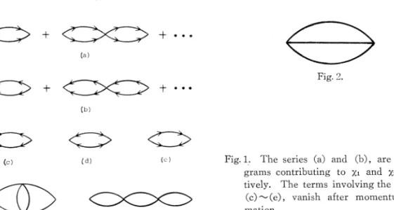
by means of thermal Green's function. Dominant contributions to

XaP

come from the perturbation series corresponding to the Feynman diagrams in Figs. 1 (a) and (b). The terms represented in Figs. 1 (c)~ (e) vanish after momentum summation. The other terms can be neglected due to a small factor of (w,/cF). That is, the term represented in Fig. 1 (f) is of order

w,/

2F compared to the term represented in Fig. 1 (g) because the interaction is restricted within the thin region around Fermi scuface.

Then we obtain X ail as follows:

<=>

+

<=:><:::=>

+ ...

(a)

<=>

+

<=:><:::=:>

+ ...

(b) (c) (d) (c) (f I (g) Fig. 1. Fig. 2.

Fig. 1. The series (a) and (b), are the dia-grams contributing to X1 and X2 respec-tively. The terms involving the diagrams

(c)~ (e), vanish after momentum sum-mation.

Fig. 2. The Feynman diagram which is taken into account for the self-energy.

(5)

776 H. Takagi and K. 1\lliyalw Xzz (Wn)

=

Xxx (Wn)

=

X1 (Wn)

+

X2 (Wn), Xzx (wn)

= -

Xxz (Wn)

=

i {Xl

(cun) - X2 (wn)}, X (w )

=

Vo

2 !1

(Wn) 1 " 6£1' 1-Vo(1-Vogn/3L12)fl(w,.) x,(w)

=

Va'

~···

f,(wn) ... . " 6£12 _1-_V₀_{(1- V}₀_{g n/3L1')}

f,

_(cu,.) where / 1 (w,.)

- T

2.:: 2.::

py'G

(p,

w,)

G (-

p, Wn ~w,), w, p J, (wn) =T

2.:: 2.::

Pv

2_G

(p,

_U),)_{G (-}_p,~wn _-wv). "'' p (16a) (16b) (17a) (17b) (18a) (18b) We can take account of the effect of collisions between quasi particles through the self-energy of th~ type in Fig. 2.

After analytical continuation of iwn from the upper half of the complex plane,

} ; , 2 (w) can be written as follows:

-GR

(~,

p,

x+ w)GR (

-~,

p,

x)] +[tanh x-W

-tanh~·]

2T

X GR

(~,

p,

x) GA(-

~'

p,

x-

w)},

(19a)

f,

(w) =

sdSJ_

S"'•

d~

soo

c{x_N

(~)

Pv

2 _{tanh _X _[GA(-

~'

p,

_x)

GA(~,

p,

_{x- w)}

4n

-w.

-oo

4nz

2T

x

GR (-

~'

p,

x)

GA

(~,

p,

x

~

w)},

(19b)

where

(20) and

N

(~) is the density of state and

r

is a collision time between quasiparticles.

It is easily seen from Eqs. (16) ~ (19) that within the approximation of par-ticle-hole symmetry X1 (w) equals X2 (w). Therefore Xzx and Xxz vanish, which means that l-vector does not precess at all. Then we expand the density of state as

(6)

(21) First of all we consider the problem near the transition temperature, that is; T~A (T), 1/r, and in the frequency region

w«;_T

which is not so strong a re-striction for practical interest near T ,. Substituting Eq. (19) r v (21) into Eq. (17),

X1.2 is reduced to (see Appendix A)

(22a)

(22b)

where

(23) and

La= N

(O)J~

J'"'

d~l_tanh_f_

8eF -w, ~ 2T

=~A~ln

2rwc

16EF2

nT ·

(24) Introduction of particle-hole assymmetry makes L0 finite which causes the l to

precess around the z-axis. So we call

L

0 an intrinsic angular momentum. From

derivation of Eq. (24), it is seen that for the whole temperature region La is given by 3 zL:;~z~ E

La=-J

k t a n h -4 '" v E3 _{2T '} (25) where

E=

JP:+

ILl~V.

Since Eq. (22) holds both in the hydrodynamical and in the collisionless region,

L0 has the same form over both regions. The expression of L0 (25) agrees with

the result by Cross7> and Nagai.6J Since La can be practically neglected due to a small factor (A/eF) 2 , we ignore it in this section.

Let us consider the structure of

x=x

1 =

x

2 in the following case.

(1) In the region A~l1/r-iwl, from Eqs. (22) and (23), we have

(w) _ 1/2

X - 9n(-iw)/(-iw+1/r) +3/4·Xarb(-iw) (-iw+1/r) +gD ' where

(26)

(7)

778 H. Takagi and

K.

}.;Jiyake and

=

(~) 1

;2 rr~N

(0) .d

Xorb 2 32T • (28)

The denominator of Eq. (26) is equivalent to Eq. (7 ·14) of L

r)

except the factor 3/4 in front of Xorb if 'f"K is regarded as

-r.

It

agrees with Nagai's6l result.

Since in the collisionless region X (rJJ) has a pole oJ0 of order of .d as we shall

see later, we consider Eq. (26) in the hydrodynamical region. Then the form of X (cv) is reduced to

(29)

which has a pole (!)0 as

9n

Wo= ---

--g n '( + 3/4 · Xorb 'f"-1

(30)

(2) In the region £1~11/-r-i(J)I (gapless region), Eq. (22) 1s reduced to

1/2

x

(w)

= - - -

--- iwrrN

(0) A

2

_j8T

+

_g

_n

(31)

Then we obtain a pole W0 as

(32)

which lies in the hydrodynamical region.

From the expressions of (29) and (31), the orbital viscosity 11 1s given by

_ {gn-r+3/4·XarbC

1 f!.-

rrN(O).d

2

/8T

for .dr-::?>1, for

.d-r

~

1 .

(33a) (33b) Outside the gapless regwn .d (T) r-)>1 or 1-

T

/Tc:::f>10-4 ,

gn-r

is much larger than Xorb'f"-1• Hence the relaxation time of lis

gn-rfgn

and proportional to (1-

T /Tc)

112

in agreement with the result of CA1l and LT.3J However in the gapless region Ll(T)r-~1, the relaxation time is rrN(O)A2

/8Tgn.

_{Since near}

Tc

_both

9n

_andA2

are proportional to (1-T

fTc),

the critical exponent of the relaxation time is zero. Next we consider the structure of X (w) in the collisionless region. From Eqs. (16) ~ (18), we obtain X (w) over the whole temperature region as (see Appendix B)

X (w)

= _l

{~.d

2 N

(0)

L:

l_tanh~(l_- ~p

2

+

p

2 2

1Apl~~)

+

_{g }}

-~.

2 2 p

E

2T

2 2 y y 4E2 - (!)2 D

(8)

It is shown in Appendix B that the denominator of 'X is the same as lhs of Eq.

(6 · 28) in LT31 _{except a dipole term.} In the low temperature limit, the expression of (34) is reduced to

(35)

In the denominator of (35), the dipole term can be neglected compared with the second term except the region

T /T

c<l0-3• Therefore 'X has a pole as

( 2

)1;2

[

2

r

.::1

J-112

OJ0

=

3 nT

ln

nT-

(36)

111 agreement vvith the result of \Volfle.'1

Near the transition temperature, we obtain 'X from Eq. (34) or Eq. (22) as (37)

Since the pole of (35) is of order of .::1, gD can be neglected except the region

(1-

T /T

c) <10-8. Thus 'X is reduced to

+-

1 (1-.Q ) 2 (1-5.Q ) 2 ln

l+.Q]}-l

- - ,

2 1-.Q (38)

where

It is easy to see that the denominator of (38) is not zero for any real oJ.

vVe find through numerical calculation that the imaginary part of the response function (38) has a peak at U) = 4/5 ·/3/2.::1 with a width of order of .::1. Therefore near the transition temperature a flapping mode is not so well defined as in the low temperature limit. From Eq. (31) where we put no restriction on

cu

but

uJ<!(T, it is concluded that a flapping mode does not exist in the gapless regiOn.

§

4. Equation of motion for the Z-vector

In this section we derive the equation of motion for l in the hydrodynamical

region.

Let us start with the Mori equation81

(9)

780

H. Takagi and K. Miyake where

iwa/3= Cla,

l,)

(l,

l);i,

(fJa/3

(s)

=(fa

(s),

f/)

(l,

l)

;i

and the random force

J"

is defined by

The scalar product

(l "'

l

~) is usually defined by

In homogeneous case the only variable to be considered 1s l because of the assumption that d does not vary. Therefore the correlation time of random forces must be much shorter than the characteristic time of l. Hence Eq. (39) becomes Markoffian,

(40)

In order to derive the coefficients of l, we make use of the identity:

. l_ __

= _

_!_(x(z) -x(O)x(o)-1 ,

z-zo)+ip(z)

z

(41)

where

and

We have obtained the response function Xa/J(co) in § 3 as follows:

=

~

t_

itLw=- Law

+9~

+ -

itLw

+~ow+

g

J

(42a) and

(42b)

(10)

where L0 and p are given by

- {gnr+3/4xorb C1

/1-

nN

(0)

1Pj8T

(see Eqs. (23) and (24)).

for for

§ 5. Concluding remarks

(43)

We have calculated the response function of l both in the hydrodynamical and m the collisionless region. The expression for "b Eq. (22), holds over the two regions. Our results are almost in agreement with others and LT's31 _{theory has} been justified in the region Llr)>1 and wr<t1. We have shown that the intrinsic angular momentum L0 has the same form over the two regions. However in the

gapless region our result is different from others; that is, the critical exponent of relaxation time of l is zero.

The approximation used in our calculation is rather simple in the hydrodyna-mical region. We have taken account of the effect of collisions between quasipar-ticles only through the imaginary part of the self-energy for the Green function. A vertex correction need not to be considered due to a small factor of ((!Jc/ cF). If we calculate the dynamical spin susceptibility within the same approximation, \Ve obtain a pure imaginary pole in the hydrodynamical region. As a result the motion of d-vector becomes relaxation not oscillation which is derived theoretical-ly9l.Iol and observed experimentally.w In calculation of the dynamical spin suscepti-bility we must consider a vertex correction.12l The difference between the orbital dynamics and the spin dynamics reflects the fact that in orbital dynamics there 1s

no local conserved variable coupled to the Z-vector such as spin density. Acknowledgements

In the course of this work we have benefited from conversations with Pro-fessor T. Usui, ProPro-fessor M. Ishikawa and ProPro-fessor Y. Kuroda.

Appendix A

Derivation of Eq. (22) from Eq. (17) -We rewrite

f

1(w) in Eq. (19a) as follows:

(11)

782

_{H. Takagi and K. 1\fiyake}

-GR

(~,

p, x)GR (

-~,

p,

x-oJ)]

+(tanhX'_--:_o)_tanh

_x

)[GR(~,p,x)GA(-~,p,x-oJ)

2T 2T

-GR

(~,

p, x)GR (

-~,

p,

x-w)J }·

(A·1)

Substituting the Green function (20) into (A ·1), the first term is reduced to

where

Near the transition temperature (T)>Ll, 1/r) and in the frequency region u)<{.._T,

(A· 2) becomes

The gap equation ,can be written in the form,

where

Using the expression for F analogous to G in Eq. (20), the gap equation is reel ucecl to

(A·4)

Subtracting (A· 4) from (A· 3), we have

11

=-+-- -

1

N

(0)

w

sw, (

d~ -tanh 1 ~ - 1 -cosh --- , _z ~ )

Va

24eF

-w,

~ 2T 2T 2T (A·5)

where we have used the form for the density of state in Eq. (21).

(12)

which is reduced to

12=-

N(O)_c~

S·clj2_

sd~py2

~~~P_I~=_(w+i/r)

2 _-

-2T 4rc

8(co+i/r)

[~2-!-IL1pl2-

(uJ-!-i/r)

2

_/4]

+}V_(O)_uJ_

S"''

d~

cosh_2

_f_.

48TeF -w, 2T

(A·6)

From Eqs. (A· 5) and (A· 6),

!

1 (co) becomes

(A·7)

Then we obtain X1 (w) in Eq. (17a) as

X1

(w)

= - · - . - 1/ 2 - - - - , (22a)

-ZUJfL(w) -Low--1-gn

where !l

(uJ)

and L0 are given by Eqs. (23) and (24). We can also derive

x

2 (cJJ)

in the same way.

Appendix B

We derive Eq. (34) and show that its denominator has the same form as Eq. (6 · 28) of LT3J except the dipole term. For this purpose we evaluate

f(rJJn) = T

I: I:

Py2_G_{(p, w,)}G (-p, _{Wn- IJJv).} (B·1) W.v ]J

After analytical continuation of iwn from the upper half complex plane, f(cu) 1s reduced to

(B·2)

where we have assumed a particle-hole symmetry. The gap equation can be writ-ten in the form

(B·3)

(13)

784

H. Takagi and K. Miyake

Performing a partial integration with respect to .Q, we obtain x(w) as fol-lows:

1/2

x

(w)

= - -

2- - - , -(J) Xorb(w) +g,.+gn (B-4) where and

The denominator of Eq. (B · 4) is cf the same form as Eq. (6 · 28) of LT. s> References

1) M. C. Cross and P. W. Anderson, Proceedings of the 14th International Conference on Low Temperature Physics, Finland, 1975, ed. M. Krusius and M. Vuorio (North-Holland, Amsterdam, 1975), vol. 1, p. 29.

2) C. I. Pethick and H. Smith, Phys. Rev. Letters 37 (1976), 226. 3) A. ]. Leggett and S. Takagi, Ann. of Phys. 110 (1978), 353.

4) P. Walfle, Quantum Statistics and Many-Body Problem, ed. S. B. Tricky, W. P. Kirk and J. W. Dufty (Plenum, New Y ark, 1975), p. 9.

5) D. N. Paulson, M. Krusius and ]. C. Wheatley, Fhys. Rev. Letters 36 (1976), 1322. 6) K. Nagai, ]. Low Temp. Phys. 36 (1979), 485.

7) M. C. Cross, ]. Low Temp. Fhys. 26 (1977), 165. 8) H. Mori, Frog. Theor. Fhys. 33 (1965), 423.

9) A. J. Leggett and S. Takagi, Ann. of Phys. 106 (1977), 79. 10) R. Combescot and H. Ebisawa, Phys. Rev. Letters 33 (1974), 810.

11) W. ]. Gully, C. M. Gould, R. C. Richardson and D. M. Lee, ]. Low Temp. Fhys. 24 (1976)' 563.