Algorithms and Data Structures for Sequence Analysis in the Pan-Genomic Era

(1)

Department of Computer Science Series of Publications A

Report A-2017-3

Algorithms and Data Structures for

Sequence Analysis in the Pan-Genomic Era

Daniel Valenzuela

To be presented with the permission of the Faculty of Science of the University of Helsinki, for public criticism in Auditorium CK112, Exactum on June 9th, 2017 at 12 o’clock noon.

University of Helsinki Finland

(2)

Supervisor

Veli M¨akinen, University of Helsinki, Finland Pre-examiners

Szymon Grabowski, Lodz University of Technology, Poland Alberto Policriti, University of Udine, Italy

Opponent

Gregory Kucherov, University Paris-Est Marne-la-Vall´ee, France Custos

Veli M¨akinen, University of Helsinki, Finland

Contact information

Department of Computer Science

P.O. Box 68 (Gustaf H¨allstr¨omin katu 2b) FI-00014 University of Helsinki

Finland

Email address: [email protected] URL: http://www.cs.helsinki.fi/

Telephone: +358 2941 911, telefax: +358 9 876 4314

Copyright c2017 Daniel Valenzuela ISSN 1238-8645

ISBN 978-951-51-3230-7 (paperback) ISBN 978-951-51-3231-4 (PDF)

Computing Reviews (1998) Classification: E.4, J.3 Helsinki 2017

(3)

Algorithms and Data Structures for Sequence Analysis in the Pan-Genomic Era

Daniel Valenzuela

Department of Computer Science

P.O. Box 68, FI-00014 University of Helsinki, Finland [email protected]

PhD Thesis, Series of Publications A, Report A-2017-3 Helsinki, May 2017, 74+78 pages

ISSN 1238-8645

ISBN 978-951-51-3230-7 (paperback) ISBN 978-951-51-3231-4 (PDF) Abstract

The advent of Next-Generation Sequencing brought new challenges for bio-logical sequence analysis: larger volumes of sequencing data, a proliferation of research projects relying on genomic analysis, and the materialization of rich genomic databases, to name a few. A recent example of the latter, gnomeAD, contains more than 15,000 whole human genomes from unre-lated individuals. Today a pressing challenge is how to leverage the full potential of such pan-genomic collections.

Among the many biological sequencing processes that rely on computa-tion methods, this thesis is motivated by variacomputa-tion calling and haplotyping. Variation calling is the process of characterizing an individual’s genome by identifying how it differs from a reference genome. The standard approach is to first obtain a set of small DNA fragments – called reads – from a biological sample. Genetic variants in the individual’s genome are detected by analyzing the alignment of these reads to the reference. A related proce-dure is haplotype phasing. Sexual organisms have their genome organized in two sets of chromosomes, with equivalent functions. Each set is in-herited from the mother and the father respectively, and its elements are calledhaplotypes. The haplotype phasing problem is, once genetic variants are discovered, to attribute them to either of the haplotypes.

The first part of this thesis incrementally builds a novel pipeline for variant calling. We propose to replace the single reference model by a pan-genomic

(4)

iv

one: a reference that comprises a large set of genomes from the same species. The first challenge to realize this goal is to efficiently handle large collec-tions of genomes. A useful tool for this task is the family of Lempel-Ziv compression algorithms. We focus on two of its exponents, namely the RLZ and LZ77 algorithms. We analyze the first, and propose some modi-fications to both. Using them we develop a scalable index that can process collections longer than 2TB.

With this pan-genomic read aligner we propose a novel variation calling pipeline to go from a single reference to thousands of them.We explore our variation calling pipeline on a mutation-rich subsequence of a Finnish population genome. Our approach consistently outperforms the single-reference approach to variation calling.

The second part of this thesis revolves around the haplotype phasing prob-lem. First, we propose a general model for sequence alignment of diploid genomes that represents diploid genomes as a pair-wise alignment. Next we extend this model to offer a solution for the haplotype phasing problem in the family-trio setting (that is, when we know the variants present in an individual and in her parents). Finally, in the context of an existing read-based approach to haplotyping, we go back to basic algorithms: we observe that the aforementioned approach needs to prune a set of reads aligned to a reference. We model this problem as an interval scheduling problem and propose an algorithm that solves the problem in sub-quadratic time. Moreover, we give a 2-approximation algorithm that runs in linearithmic time.

Computing Reviews (1998) Categories and Subject Descriptors:

E.4 Coding and Information Theory: Data compaction and compression

J.3 Life and medical sciences: Biology and genetics General Terms:

Algorithms, Design, Experimentation Additional Key Words and Phrases: Sequence alignment, Pan-genomics

(5)

Acknowledgements

I could not have made it this far without the support of many people to whom I am deeply thankful.

First and foremost, to my supervisor, Professor Veli M¨akinen: thank you for trusting me, for sharing your way of doing research, and for the opportunity to work in exciting problems. Thank you for the freedom and for the guidance you gave me throughout this four-year journey. I was also fortunate in my other mentors on this journey: Alexandru I. Tomescu, Travis Gagie and Simon J. Puglisi. Thank you for your time, patience and guidance. I would also like to express my sincere gratitude to the present and past members of the Genome-scale algorithmics for creating a fantastic working environment.

I would also like to thank the institutions that have supported this research: The Centre of Excellence in Cancer Genetics (CoECG), funded by the Academy of Finland, the Doctoral Programme in Computer Science (DoCS), the Department of Computer Science of the University of Helsinki, and the Helsinki Institute for Information and Technology (HIIT).

This manuscript is based on a series of papers, and I am thankful to all of my co-authors; it was a pleasure to work together with you. I would also like to thank my pre-examiners Szymon Grabowski and Alberto Policriti, for reading the entire thesis and providing helpful feedback. Thanks to Iona Italia and Pirjo Moen too, for their help with the manuscript.

It is thanks to Gonzalo Navarro that I ended up in Helsinki: thanks for encouraging me to take this leap, it was totally worth it!

After my M.Sc I was exploring possibilities for the future and I was lucky enough to encounter excellent mentors, whose advices and teaching were lasting and helped me to get through this PhD. For this I owe a special debt of gratitude to Professor Hannah Bast and to Andres Villavicencio.

Finally, but most importantly, I want to thank my friends and loved ones. My gratitude to you may have nothing to do with this thesis, but friendship is the most important thing in life and I am grateful for yours. I particularly like to thank my parents, Alejandro and Tili, for

(6)

vi

cally supporting me in every endeavour. Finally I would like to thank my wife Nadia, for bravely joining me in this great adventure of love. As we build a life together you have made my life richer than ever.

Helsinki, May, 2017 Daniel Valenzuela

(7)

Original Papers

This thesis is based on the following research articles, referred as Paper I to Paper VI in the thesis.

I Daniel Valenzuela. CHICO: A Compressed Hybrid Index for Repetitive Collections. In Proc. 15th Symposium on Experimental Algorithms (SEA 2016).

II Travis Gagie, Simon J. Puglisi, and Daniel Valenzuela. Analyzing Relative Lempel-Ziv. In Proc. 23rd International Symposium on String Processing and Information Retrieval (SPIRE 2016).

III Daniel Valenzuela, Niko Välimäki, Esa Pitkänen and Veli Mäkinen. Pan-Genome Read Alignment to Improve Variation Calling. Submitted.

IV Veli M¨akinen and Daniel Valenzuela. Recombination-aware align-ment of diploid individuals. In BMC Genomics 2014 15(Suppl 6):S15

V Veli M¨akinen and Daniel Valenzuela. Diploid Alignments and Haplotyping. In Proc. 11th International Symposium on Bioinfor-matics Research and Applications (ISBRA 2015).

VI Veli M¨akinen, Valeria Staneva, Alexandru I. Tomescu, Daniel Valen-zuela and Sebastian Wilzbach. Interval scheduling maximizing minimum coverage. InDiscrete Applied Mathematics. Volume 225, 2017.

(8)

(9)

Chapter 1 Introduction

The first drafts of the Human Genome were published in 2001 [47, 94]. Obtaining them was a multi-billion dollar enterprise that involved over 20 institutions in 6 countries and hundreds of researchers [18].

In contrast, during the 2010s we have witnessed a growing market for personalized genomes: it is possible to send a sample of blood or saliva by mail and get your results on-line, for prices ranging between less than a hundred to the couple of thousand dollars.1

Despite the many technological advances since the completion of the Human Genome Project, two factors are crucial to explain such a drop in prices: first, the adoption of the so called Next-Generation Sequencing tech-nologies made a huge impact on decreasing the sequencing costs; second, once the first human genome is obtained, the process to sequence a new individual’s genome changes entirely. The first time, the sequence needs to be assembled “from scratch”. From then onwards, the first sequence can be used as areference for a much accessible process called variation calling (see Section 1.2).

Today the landscape keeps changing: there are thousands of high-quality genomes available [89] and more are being sequenced [90, 27], estab-lishing a map of genetic diversity in the search for a better understanding of its implications. Similar processes have been ongoing also for non-human organisms [87, 84], to the extent that some authors talk about the dawn of thepan-genomic era[19].

All those achievements have been heavily reliant on computational meth-ods [70, 41, 26]. There is a large repertoire of those methmeth-ods that are critical

1 _{The current diversity of prices is due to many factors, including how much of the}

total genome is actually sequenced. The startup 23andMe famously offered genomes from less than $100USD, mainly focusing on specific sites in the genome. On the other hand, Illumina offers whole-genome sequencing for $5,000USD[92].

(12)

2 1 Introduction

for different stages of the genome sequencing processes. As the sequenc-ing technologies are advancsequenc-ing rapidly, the computational methods need to advance as well, evolving and adapting to new challenges. In this thesis I will present different algorithms and data-structures aiming to contribute to some of these processes needed for genome sequencing. In particular, some of the contributions consider the pan-genomic nature of the data we now have available.

The structure of this chapter is as follows: In Sections 1.1 and 1.2 I will introduce some basic concepts from bioinformatics. Then in Section 1.3 I will outline this thesis’ contributions. Finally, in Section 1.4 I give a brief summary of the original publications, discussing my personal contribution to each of them.

1.1 DNA and genetic variation

Deoxyribonucleic acid (DNA) constitutes “the blueprints of life”, for it is the molecule within the cell that contains the instructions for growing, func-tioning and reproducing for all known living organisms. A DNA molecule is the linear concatenation of nucleotides, which can be of four different kinds: adenine(A), cytosine(C), guanine(G) and thymine(T). Most of the DNA is packed in units calledchromosomes. Different species have different numbers of chromosomes with different contents. Within species, different individuals normally have the same number of chromosomes and the con-tent of each chromosome is highly similar throughout the population.

In most cells of sexual organisms, chromosomes are organized in pairs, such that each element of the pair – a “copy” – is inherited from a “father” and a “mother” respectively. Each of those copies are called homologous chromosomesorhaplotypes. The cells that have this arrangement are called diploid cells. During reproduction, specialized cellsrecombine the pairs of chromosomes generating gametes: cells that have only one copy of each chromosome and that later can combine with a gamete from another in-dividual to create a new inin-dividual. These replication and recombination processes are not exact, and sometimes an “error” occurs, generating ge-netic variations that can be later inherited by the offspring.

Because most of the genetic content is the same among individuals within the same species, it is possible to define a reference genome for a species. Then, we can characterize thegenetic variations of each individual in terms of how they differ from the reference genome. A variant that occurs in a single nucleotide, where, for instance a specific T in the reference genome is replaced by a G, is called single nucleotide polymorphism (SNP),

(13)

1.2 NGS and variation calling 3 or single nucleotides variants (SNV). Those account for a large amount of the known variations in human genomes, however there are also more complex variants such as (large) insertions, deletions, inversions, among others. When a variant is present in only one of the chromosome copies, it is said to be a heterozygous variant. A variant that is present in both copies is known as ahomozygous variant.

1.2 NGS and variation calling

Next-Generation Sequencing (NGS) is an expression that refers to many technologies that have parallelized the sequencing process, producing vast amounts of sequences concurrently. What these have in common is that they cut DNA molecules from the donor into small pieces, known asreads, which are what is actually sequenced in great amounts. Reads length can range from about a hundred to a couple of thousands nucleotides. When reads are sequenced there is no information about their original position in the genome, so the output is essentially a large set of small pieces of the genome.2 The problem of sequencing a genome starting from this set of reads is known as de novo genome assembly. This is known to be a hard problem, and its simplest mathematical formulation is NP-Hard [67].

When we already posses a reference genome of the same species as the donor, the enterprise to sequence the donor genome is much more accessi-ble through what is known as variation calling. A simplified summary of this process is as follows: Starting from a biological sample from the donor, NGS technology is used to obtain a massive set of reads. A read aligner maps the reads to the reference genome, ideally to positions with a high similarity score with the read. The number of reads whose alignment covers a position is known as thecoverage. As the number of NGS reads is large, the ideal situation is to have high coverage through the genome, so that any position on the reference genome will have many reads piled up. This pile-up is analyzed, typically using statistical methods [59, 36] that can discover variations in the donor genome. With this process SNPs are rel-atively easy to detect, but more complex variants pose a bigger challenge. Nowadays, variation calling is routinely performed to sequence genomes, using a wide variety of methods [4, 59, 85, 74]. However, their results are not always consistent [74]. This in itself is motivation enough to study possible improvements for variation-calling mechanisms.

2

There is more information, for instance, each base is annotated with the error probability, and some technologies havepaired-endreads, where there is a prior knowledge about their expected distance within the genome.

(14)

4 1 Introduction

When variation-calling tools report a variant, they will indicate whether it is homozygous or heterozygous. However, this is not enough to com-pletely reconstruct the donors genome: we still do not know to which of the two copies of each chromosome each variant belongs to. The problem of deciding whether two variants belong to the same copy of the chromosome or not is called haplotype phasing. There is a wide repertoire of methods to address this problem [13, 14, 10, 76]

1.3 Outline of the contributions

The main motivation of this thesis is found in variation calling and hap-lotype phasing. Our contributions are at different levels, from analysis of basic algorithms, to the design of novel pipelines for variation calling.

The first part of this thesis incrementally builds a novel framework for variant calling. We propose to replace the single reference model by a pan-genomic one: a reference that comprises a large set of genomes from the same species. The second part revolves around the haplotype phasing problem. In Chapter 2 we first review the basic algorithms that we will use throughout this thesis.

The first challenge in the route to the pan-genomic reference, is to ef-ficiently handle large collection of genomes. A useful tool for this is the family of Lempel-Ziv compression algorithms, which have proven to be extremely effective to compress highly repetitive collections, such as collec-tions of genomes from the same species. In Chapter 3 we introduce two exponents of this algorithms: the LZ77 and the RLZ algorithms. Then, we present the contributions of Paper I: a study of the functioning of the RLZ in a particular setting, namely, the construction of an artificial reference.

Then, in Chapter 4 we propose a slight generalization of the LZ77 al-gorithm so that we obtain a class that includes the LZ77 and the RLZ algorithms. Utilizing this we develop a scalable index that can process a 2.4TB synthetic collection of DNA in less than 12 hours.

To improve variation calling, in Chapter 5 we submit a novel pipeline that replaces the single linear reference by a pan-genomic one. To index the pan-genome we further develop the index of Chapter 4 to transform it into a read aligner for pan-genomic reference. This chapter is based on the work of Paper III. We tested our read aligner on real data, replacing the standard reference by sequences from the 1000 genomes project. The use of this pan-genomic reference increased the number of mapped reads, while the time required for the mapping remained in the same ballpark. We tested our variation calling pipeline on a mutation-rich subsequence of

(15)

1.4 Original papers and individual contributions 5 a Finnish population genome, and observed that the results are better than a standard variation calling pipeline.

The first contribution of Chapter 6 is a general model for sequence alignment of diploid genomes, which represents diploid genomes as a pair-wise alignment. This is based on Paper IV, where we originally proposed this model. Then, we extend this representation to model the haplotype phasing problem in the so called family-trio setting (that is, when we know the variants present in an individual and in her parents). This latter part of Chapter 6 is based on Paper V.

Finally, in the context of an existing read-based approach to haplotyp-ing [76], in Chapter 7 we go back to basic algorithms. We observe that the aforementioned approach needs to prune a set of reads aligned to a reference, and in the original solution the reads were randomly pruned. We studied this pruning problem and its motivation, modeled it as an inter-val scheduling problem, and propose exact and approximate algorithms to solve it.

Finally, Chapter 8 summarizes the contributions, discussing open prob-lems and possible directions for future research.

1.4 Original papers and individual contributions

Next I give a brief summary of the original papers that are the basis of this thesis, indicating my specific contribution in each of them.

Paper I.In this paper we presented a theoretical and empirical study on the compression achieved by the Relative-Lempel Ziv algorithm in the scenario where it needs to build an artificial reference.

My contributions to this work were in the experimental study: the experimental analysis was jointly designed by the three authors. I imple-mented and ran the experiments and contributed to the writing of that section.

Paper II.In this paper I presented CHICO, an improved version of the Hybrid Index of Ferrada, Gagie, Hirvola and Puglisi [29]. CHICO reduces the space usage of the original version while keeping similar query times. Compared with other indexes for repetitive collections, the size of the index and query times were competitive, while indexing times were better than all the alternatives. In this paper I also demonstrated the scalability of the approach, which indexed a 2.4TB collection in about 12 hours.

(16)

6 1 Introduction

Paper III. In this paper we proposed a novel framework to perform variation calling using pan-genomic references and released an implementa-tion called PanVC. We represent the pan-genome using a multiple sequence alignment, indexing the underlying sequence using CHIC aligner, a special-ized version of the index of Paper II. We demonstrated that the approach can improve the effectiveness of variation calling.

The framework was jointly designed with Veli M¨akinen. I implemented PanVC and the CHIC aligner. I ran all the experiments for PanVC and wrote a significant part of the paper.

Paper IV. In this paper we proposed a generalization of edit dis-tance/sequence alignment where the object to be aligned is itself a pair-wise alignment. The proposal is to model diploid individuals as pair-pair-wise alignments instead of a single sequence. This captures the possibility of known variants whose correct haplotype phase is not known or that has been wrongly phased.

The original idea is from Veli M¨akinen, the actual model and algorithms were jointly designed. I implemented the algorithms and ran the experi-ments, and the paper was written jointly.

Paper V. This is a follow-up of Paper IV, where we extended the diploid alignment model to solve the haplotyping problem in family trios, that is, when the genome has been sequenced but not phased for a father, a mother and a child.

The model and algorithm were done jointly. I implemented the algo-rithms and ran the experiments, and the paper was written jointly.

Paper VI. In this paper we addresses the problem of pruning a set of NGS reads aligned to a reference. This step is a required preprocessing step needed by previous approaches to the haplotyping problem [62, 76]. We modeled it as a job scheduling problem and present different algorithms to solve it.

The exact algorithms were designed together by Veli M¨akinen, Alexandru Tomescu and me. I also contributed with the analysis of the 2-approximation algorithm, and with the supervision of Sebastian Wilzbach, who implemented the exact algorithm and ran the experiments.

(17)

Chapter 2 Preliminaries

In this chapter we introduce some basic concepts in computer science that will be used through this thesis.

2.1 Strings

Astring is a finite sequence of characters over an alphabet Σ ={1,2, .., σ}. We denoteS[1..n] a string of length n, and we use S[i] to signify the i-th character ofS. We denote by S[i..j] a substring of S starting at positioni until positionj, both inclusive. Any substringS[1..i] (starting from the first character) is called aprefix of S, and any substring S[i..n] (including the last character) is called asuffix ofS. We say thatT is asubsequenceofS if we can obtainT by deleting any number of characters from S. Conversely, we say thatS is asupersequence ofT.

For example,S =GAT T ACAis a string of length 7, andS[3..5] =T T A is a substring of S and T = GT T C is a subsequence of S obtained by eliminating the second, fifth and seventh characters. S[5..7] = ACA is a suffix ofS and S[1..4] =GAT T is a prefix of S.

2.2 Edit distance and sequence alignment

There are many definitions of distances between two strings. A simple, yet versatile definition isedit distance, defined as the minimum number of edit operations required to transform one string into the other. Different sets of allowed operations lead to different distances. For instance, the Levenshtein distanceconsiders substitutions, deletions and insertions as the possible operations. It is possible to generalize the Levenshtein distance by

(18)

8 2 Preliminaries

assigning different costs to each operation and then defining the distance as the minimum-cost required to transform one string into the other.

A closely related concept is sequence alignment. A pair-wise alignment (or simply an alignment, when it is clear from the context) of A and B is a pair of sequences (SA_,_SB_{) such that} _SA _{is a supersequence of} _A, _SB

is a supersequence of B, _|SA_| = _|SB_| = n is the length of the alignment, and all positions which are not part of the subsequenceA (respectively B) in SA (respectively SB), contain the gap symbol 0₋0, which is not present in the original sequences. Given a cost function C(a, b) to transform the characterainto b, the cost of a pair-wise alignment is defined as

S(SA,SB) =

n X

i=1

C(SA[i],SB[i]).

The weighted edit distance is defined as

S(A, B) =min_{

n X

1=1

C(SA[i],SB[i]) : (SA,SB) is an alignment of Aand B_}.

An alignment that achieves that value is called an optimal alignment. It is possible to use asimilarity function instead of a cost function, in which case the minimum is replaced by a maximum, and the resulting measure is thesimilarity between strings A and B. A rich variety of models exist, considering inversions, translocations, non-linear costs for gaps, etc [26].

2.3 Graphs and trees

A directed graphG= (V, E) is a pair of sets comprising the set ofvertices V ={v1, v2, . . . , v|V|} (also called nodes) and the set of edges E ⊆V ×V (also called arcs). An edge (u, v) _∈E is called an arc from u tov and we say that u and v are adjacent. When we consider (u, v) _≡ (v, u) we say that the graph isundirected, otherwise we call it a directed graph.

A path of lengthp is a sequence of nodes u1u2. . . up such that

consec-utive nodes are connected by an arc, i.e. for all 1 _≤ i < p it holds that (ui, ui+1)∈E. We say thatu1 and up areconnected. Acycle is a path of

length at least two from a node to itself. A graph that contains no cycle is calledacyclic.

A tree is a graph where any two vertices are connected by exactly one path. A rooted tree is a graph when a specific node is designated as root. Unless stated otherwise, we will assume all the trees are directed and rooted.

(19)

2.4 Flow networks 9

2.4 Flow networks

A flow network is a directed graph where the edges have acapacity c(u, v) and can be assigned a flow value f(u, v) ≤ c(u, v) Some vertices can be designated assources and some others can be designated as sinks.

A valid flow is characterized by the flow conservation property: the total amount of flow entering a node must be equal to the total amount of flow exiting the node, with the exception of sources, which only have outgoing flow, and sinks, which only have incoming flow. More precisely for all nodesu_∈V that are neither a source nor a sink, it holds that

X

(x,u)∈E

f(x, u) = X

(u,y)∈E

f(u, y)

The maximum flow problem is, given a flow network, find a valid flow that is maximum. A classical solution to the max-flow problem is the Ford-Fulkerson algorithm [35], which relies on the notion of residual net-work. Given a network (G, V), the residual network (Gr, Vr) is the network

with the same nodes and edges, capacitiescr(u, v) =c(u, v)−f(u, v) and

fr(u, v) = 0. The Ford-Fulkerson algorithm finds an augmenting path in

the residual network and adjusts the flow network along the same path so as to increase the total flow. When there is no augmenting path left in the residual network, the flow found is maximum. Assuming integral capacities (so that the flow increases at least by one unit each augmentation step), the running time is O(|E||ϕ∗|), whereE is the set of arcs of the flow network and_|ϕ∗_|_{is the value of the maximum flow.}

2.5 String matching and text indexing

Given a text T[1..n] and a pattern P[1..m], typically with m n, the string matching problem is to find all the occurrences ofP in T. This is sometimes called a locate query, while a count query is only to find the number of such occurrences, and an existential query asks whether this number is zero or not.

When the text is available for preprocessing the scenario is known as indexed string matching. Sometimes these indexes are called full-text in-dexesto highlight their difference from the indexes used in natural language that assume a text made of words or other structures. In this section we will assume, without loss of generality, that the textT[1..n] is terminated with a unique character T[n] = $ which is lexicographically smaller than

(20)

10 2 Preliminaries

any other character.1 In the following we review the foundational full-text indexes.

2.5.1 Suffix tree

A trie is a tree used to represent a set of strings. Each edge is labeled with a character, and for every node no two out-going edges can have the same label. Then each nodevuniquely represents the string spelled by the path from the root tov. It follows that if a stringS is represented by a nodev in the trie, then all the prefixes of S are also represented, precisely by the nodes in the path from the root tov.

A suffix trie is a trie where all the leaves represent the suffixes of the text. All the proper substrings of T are represented by an internal node. Given a text T[1..n] and a query pattern P[1..m], the suffix trie of T can be used to solve the string matching problem as follows: starting from the root, if there is no edge labeled withP[1] we know that P does not occur inT. If such an edge exists, we descend through it and repeat the process for P[2] and so on until P[m]. If at the end of this process we are in a node, all the leaves that are reachable from that node corresponds to the positions inT whereP occurs. The suffix trie usesO(n2_log_{n) bits, and it}

can solve the string matching in timeO(|P|).

The suffix tree [96] is a compressed representation of the suffix trie, where all the unary paths are compacted, and the edges are labeled with the corresponding strings, encoded as a pair of pointers to the text. The resulting data structure requiresO(nlogn) bits of space and it solves the counting problem in O(_|P_|) time and the locate problem in O(_|P_|+occ) time assuming a constant size alphabet, in which case both of the times are optimal.

2.5.2 Suffix array

The suffix array [65] of T, is the permutation of [1..n] that corresponds to the lexicographical order of the suffixes of T. More formally, it holds thatT[SA[i]..n]< T[SA[i+ 1]..n]. It is worth noting that the suffix array corresponds to the values in the leaves of the suffix tree from left to right. The suffix array uses ndlogne bits and offers a functionality similar to that of the suffix tree, with a moderate slowdown: counting the occurrences

1 _{Assuming that the strings terminate with the special symbol $, lexicographical}

smaller than any other character, is commonly adopted to avoid the special case when a suffix is a prefix of another suffix. For instance, this is needed to guarantee that the suffix trie ofT[1..n] has exactlynleaves.

(21)

2.6 Compressed full-text indexes 11 of P can be done in O(_|P_|logn), and reporting their occ locations takes O(_|P_|logn+occ) time.

Compared to the suffix tree, the suffix array significantly reduced the space usage, however, in certain domains the n_dlogn_e bits are still pro-hibitive.

2.6 Compressed full-text indexes

The quest for reducing the space usage of the indexes took a big leap with the development of compressed full-text indexes. Here, the indexes take advantage of the compressibility of the text itself, and the goal is to obtain indexes whose space requirement is proportional to the size of the compressed representation of the text, while still providing the search capabilities of the indexes mentioned in the previous section. Another way of seeing this is as a compressed representation of the text that can be rapidly searched.

There are many approaches to design compressed full-text indexes. For instance, it has been noted that repetitions in the text translate into runs in the suffix array, which can be exploited to compress it. Manycompressed suffix arrays have been developed based on this and similar ideas [39, 6, 72]. A related although different approach is based on the Burrows-Wheeler Transform (BWT), which was originally designed for text compression. The BWT is a reversible transformation of the text which usually is easier to compress than the text itself [12]. Later, Ferragina and Manzini discovered that the BWT can be used to solve the string matching problem [30]. It is possible to emulate the suffix array using the BWT to find the suffix array interval corresponding to the occurrences of the query pattern.

There is a large family of FM-Indexes, depending on the precise repre-sentation of the BWT and other supporting data structures. For instance, the alphabet-friendly FM-index [32] requiresnHk(T) +o(nlogσ) bits2 and

it can count the occurrences of P in T in time O(_|P_|logσ). For detailed descriptions and different approaches to compressed text indexes we refer the reader to a comprehensive survey [72].

2

Hk(T) is the kth-order entropy ofT, and nHk(T) is the space in bits used by a

statistical compression model that uses contexts of lengthk. In the worst case (random text),Hk(T) = logσand this term is equal to the plain encoding of the text.

(22)

(23)

Chapter 3 Analysis of Relative Lempel Ziv

with Artificial References

Almost forty years have passed since Abraham Lempel and Jacob Ziv pub-lished the so-called LZ77 and LZ78 algorithms [100, 101]. Today, they remain central to data compression: Those algorithms and their deriva-tives are at the core of widely used compression tools like zip, gzip, 7zip, image formats like GIF and PNG, and also in modern libraries like Brotli and Zstandard used to speed-up web browsing.

These algorithms are still actively researched [2, 7, 34, 25], and new variants are still being proposed to address new challenges [51, 56]. Rel-ative Lempel Ziv (RLZ) [56] is a recent variation of LZ77 that has been particularly successful in the compression of highly repetitive collections.

In this section we review the contributions of Paper I, where the com-pression achieved by using RLZ with artificial reference construction is analyzed both from a theoretical and from a practical perspective.

3.1 LZ77 and Relative Lempel Ziv

In the literature there are slightly different versions of the LZ77 parsing. We will adopt the following one: given a textT[1..n], the LZ77 parsing ofT is a partitioningT =T1_T2_{. . . T}z_{such that for 1}_≤_i_≤_{z, with}_p

i=Pij−=11 |Tj|

it holds that either:

• Ti _{is a character that does not occur in}_T_[1..p i] or

• Ti _{is the longest string that is simultaneously a prefix of}_T_[p

i+ 1..n]

and a substring T[1..pi]

(24)

14 3 Analysis of RLZ with Artificial References

We will call the former literal phrases and the latter copying phrases. Both types of phrases can be represented as pair of integers (pos, len). For copying phrases, posis the position in T[1..pi] in which Ti occurs and

len= _|Ti_| _{is its length. For literal phrases} _pos _{= 0 and} _len _{is the binary}

representation of the new character.

The above definition is sometimes referred to as greedy LZ77 parsing because, parsing from left to right, the next phrase is always the longest possible. The greedy parsing always produces the minimum number of phrases [78], however, when the output size is considered under different encoding schemes, more sophisticated non-greedy parsings are needed to achieve optimality [33].

Although several linear-time algorithms for computing the LZ77 pars-ing are known (c.f. [78]), there is ongopars-ing research on how to improve the practical efficiency [50, 49]. An important challenge is the scenario where the text to be processed is too big to fit in memory. One strategy is to make efficient use of external memory [51]. Another is to introduce changes into the algorithm, such as a user-defined parameter to bound the distance be-tween a phrase and its source. This approach, known asfixed window LZ77, has been used since the early days of Lempel-Ziv algorithms, and it remains present in popular tools such gzip. However, when the repeated substrings are too distant in the text, this model will achieve little compression.

In 2010, Kuruppu, Puglisi and Zobel introduced Relative Lempel Ziv (RLZ), a novel variation of LZ77 originally designed for compression of genomes. In RLZ, in addition to the text to be compressed, there is another text called the reference (or the dictionary), which is expected to be much shorter than the text. Similar to LZ77, the text is greed-ily parsed into phrases, but now the phrases correspond to occurrences in the dictionary instead of the text itself. More precisely, given a text T[1..n] and a dictionary D[1..d], and assuming that T[1..i−1] has already been parsed, the next phrase corresponds to the largest T[i..j] such that T[i..j] =D[pos..pos+j₋i+ 1] for somepos. The dictionary is also part of the output, and the phrases can be codified as pairs (pos, len) analogously to LZ77.

3.2 Artificial reference for RLZ

In collections where all the documents are highly similar to each other, taking any of the documents as a reference should produce a decent level of compression. Paradigmatic examples of this are genomic databases where all the stored sequences are individuals from the same species. However,

(25)

3.3 Theoretical analysis 15 there are datasets that are still highly compressible but without such a homogeneous structure. In the latter setting, it is possible to build an artificial reference[44], by sampling substrings from the entire dataset and concatenating them. This approach has exhibited excellent performance in practice [44, 91, 61].

In the following sections we review the contributions of Paper I, where we analyzed the functioning of RLZ compression using artificial reference.

3.3 Theoretical analysis

We begin with an intuitive view about the artificial reference RLZ. Con-sider a somewhat short substring of the text: on the one hand, if it is frequent enough it is likely to be sampled and thus be part of the reference. Therefore, all its occurrences can be represented as a single pair (pos, len) and will use little space. On the other hand, if it is not so frequent all its occurrences can be encoded literally without consuming much space. The rest of this section presents a formal analysis of this reasoning.

Consider a string T[1..n] over an alphabet of size σ whose LZ77 parse consists of z phrases. Given integers k and `, let us sample k substrings of length ` from T and concatenate them, appending the first and last ` characters ofT, to obtain the reference. This takesO(k`logσ) bits.

For our analysis we use a partition of T into _O(n/`) blocks of length at most `/2 such that O(zlogn) of them are distinct, for 2 ≤ ` ≤ n. A previous result by Gawrychowski [37] shows that such a partition exists when there is a grammar of size zlogn that represents T; moreover, it is possible to obtain such a grammar from the LZ77 representation ofT [83]. Let us consider theith distinct block, whose frequency isfi. The

prob-ability that one of its occurrences is completely included in some of the sampled substring is at least 1−pi, wherepi =

1−fi`

2n k

. In that case, all of its occurrences are stored using _O(filog(k`)) bits in total. Otherwise,

they are stored literally using_O(fi`logσ) bits.

Letb=_O(zlogn) be the number of distinct blocks. The expected size in bits of the RLZ parse is:

O b X i=1 fi(1−pi) log(k`) + b X i=1 fipi`logσ ! ≤ O nlog(_`k`)+`logσ b X i=1 fipi !

(26)

16 3 Analysis of RLZ with Artificial References Since 1−x ≤ e−x_{, we have} _p i = 1−fi` 2n k ≤ 1 efik`/2n so Pb i=1fipi ≤ Pb i=1 fi

efik`/2n, which is concave and, thus, maximum when all the distinct

blocks occur equally often. Therefore, calculation shows

`logσ b X i=1 fipi= nlogσ eΩ(k/zlogn).

Summing up, we obtain the following theorem:

Theorem 3.1 (Paper I) If we randomly sample and concatenatekblocks of length`from the dataset to form an artificial reference, then the expected total size in bits of the RLZ encoding (i.e., the reference and the parse together) is bounded by O k`logσ+nlog(k`) ` + nlogσ eΩ(k/zlogn).

It follows that the following conditions guarantee good (expected) com-pression:

1. k`n,

2. log(k`)`logσ, 3. k=ω(zlogn).

The first condition states that the reference should be sufficiently smaller thanT. The second condition states that a pointer to the reference should be sufficiently smaller than the literal encoding of the string that it is repre-senting. The third condition is more interesting, as it reveals an asymmetry: choosing k, say, a tenth larger than optimal should not increase the size of the encoding by more than about a tenth, however, choosing ka tenth smallerthan optimal could drastically worsen compression.

A careful selection of the sampling valueskand`leads to the following result:

Corollary 3.1 (Paper I) If we randomly sample and concatenate k = zlog2+n blocks of length ` = pn/k, then the expected total size of the RLZ encoding is_O (nz)1/2_log2+_n

Which shows that if LZ77 compress well, then RLZ with an artificial refer-ence can compress well too.

(27)

3.4 Experimental analysis 17

3.4 Experimental analysis

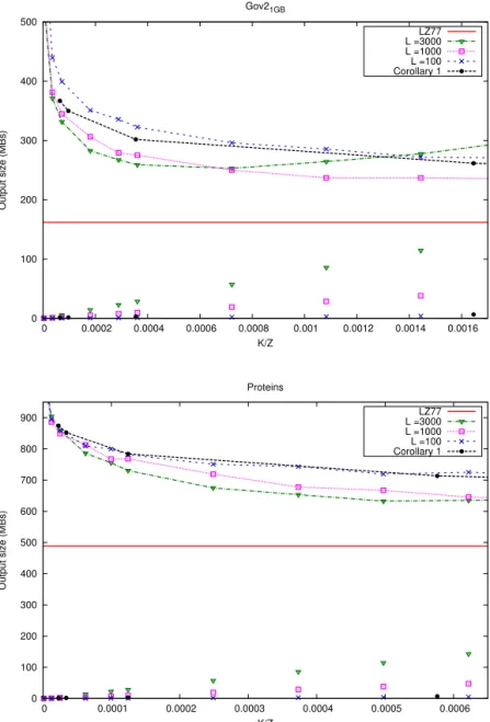
In our experimental study, we considered different 1GB collections con-taining web crawls, protein sequences or synthetic datasets. Their detailed description is given in Paper I. We built an artificial reference by picking values ofk and ` and then concatenating k randomly sampled substrings of length`from the dataset, storing the resulting reference in k`logσ bits. Then we ran the RLZ algorithm, and stored the phrases using log(k`) bits for pointers and log`bits for phrase lengths. We used two different regimes to choose thekand `values:

• Fixed length used a fixed a value of`and tried different values ofk. • Corollary 1 used the values of k and` prescribed by Corollary 3.1,

using varying estimates of z.

The points representing the total size for each sampling scheme are con-nected by lines, and below each of them we plot an extra point representing the size used only by the reference. As a baseline, we included the size of the LZ77 encoding using 2 lognbits for each phrase.

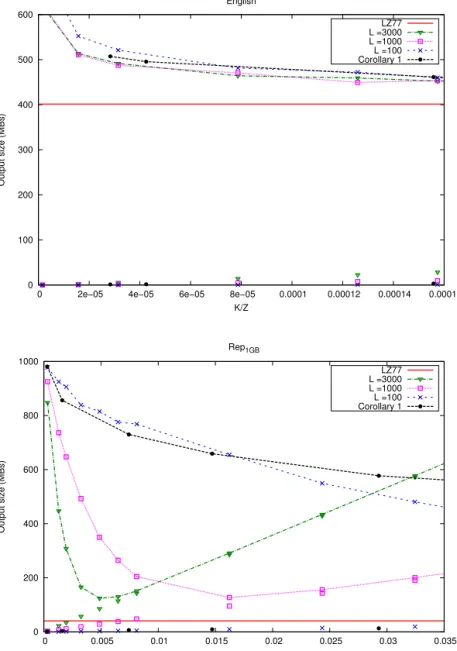
In Figures 3.1 and 3.2 we reproduce the results from Paper I. The curves we obtained are in accordance with Theorem 3.1: there is a sharp drop on the left, corresponding with the expected damage to compression by using too smallkvalues. In this area increasing the number of samples significantly improves compression. At some point, the curves start to rise roughly parallel to the reference size, which increases linearly. This improves the understanding of why the reference pruning [91, 61] approach works: it is much safer to oversample in the beginning than to undersample.

(28)

18 3 Analysis of RLZ with Artificial References 0 100 200 300 400 500 0 0.0002 0.0004 0.0006 0.0008 0.001 0.0012 0.0014 0.0016 Output size (MBs) K/Z Gov2_1GB LZ77 L =3000 L =1000 L =100 Corollary 1 0 100 200 300 400 500 600 700 800 900 0 0.0001 0.0002 0.0003 0.0004 0.0005 0.0006 Output size (MBs) K/Z Proteins LZ77 L =3000 L =1000 L =100 Corollary 1

Figure 3.1: Size in bits of RLZ compression using different artificial references on two 1GB collections: Gov21GBis part of a web crawl from the TREC collection, and Proteins

is a set of protein sequences obtained from the Swissprot database. Different regimes for constructing the reference are shown for each collection: fixed length of samples of size 3000, 1000, and 100 characters each, and varying amounts (k value) for each of them. The strategy proposed by Corollary 1 is also used. The curves show the total size of the encoding as a function ofk/z. The red horizontal line is the size of the LZ77 encoding as a baseline.

(29)

3.4 Experimental analysis 19 0 100 200 300 400 500 600

0 2e−05 4e−05 6e−05 8e−05 0.0001 0.00012 0.00014 0.00016

Output size (MBs) K/Z English LZ77 L =3000 L =1000 L =100 Corollary 1 0 200 400 600 800 1000 0 0.005 0.01 0.015 0.02 0.025 0.03 0.035 Output size (MBs) K/Z Rep_1GB LZ77 L =3000 L =1000 L =100 Corollary 1

Figure 3.2: Size in bits of RLZ compression using different artificial references on two 1GB collections: English is a concatenation of English text from the Gutenberg Project, and Rep1GB is a very repetitive synthetic file made of 400 copies of a random 25MB

string. Different regimes for constructing the reference are shown for each collection: fixed length of samples of size 3000, 1000, and 100 characters each, and varying amounts (kvalue) for each of them. The strategy proposed by Corollary 1 is also used. The curves show the total size of the encoding as a function ofk/z. The red horizontal line is the size of the LZ77 encoding as a baseline.

(30)

(31)

Chapter 4 CHICO: A Compressed Hybrid

Index for Repetitive Collections

Given a text T[1..n] and a query pattern P[1..m], the string matching problem is to find all the occurrences ofP inT. This is a central problem in computer science, and the variant whereT is available to be preprocessed is called theindexed pattern matching problem.

Since it became evident, in the 80s [17], that indexed string matching is relevant for analysing biological sequences, bioinformatics has played an important role in pushing the development of the field. To increase applica-bility of index data structures there has been a continuous effort to reduce their size while retaining strong search capability. A classic example is the Suffix Array [65], which uses much less space than the Suffix Tree [96], and can provide the same functionality when augmented appropriately [1]. This trend has led to the development of a whole research area,compressed in-dexing [72], where the idea is to build an index that uses space proportional to a compressed representation of the text. Particularly important results, like the FM-Index [30, 31], are based on the Burrows-Wheeler transform (BWT) [12]. Those indexes are currently at the heart of widely-used read aligners such as BWA [60] and BowTie2 [57].

A recent trend in this context is indexingrepetitive collections. The mo-tivation again is nurtured from bioinformatics: projects like 1000 genomes and UK10K are examples of highly repetitive collections where providing pattern matching functionalities can be valuable.

In this chapter we present CHICO, the contribution of Paper II. CHICO is a compressed index for approximate string matching that combines Lempel-Ziv algorithms with the FM-Index to efficiently handle very large and repetitive collections.

(32)

22

4 CHICO: A Compressed Hybrid Index for Repetitive Collections

4.1 Kernelization

CHICO is an improved version of the Hybrid Index of Ferrada, Gagie, Hirvola and Puglisi [29]. Their strategy is to find akernel string that is, on a highly repetitive collection, much shorter than the input text and that it is also enough to solve the approximate pattern matching problem in it.

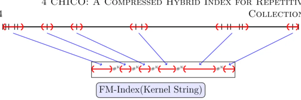
This index takes as an input the text, its LZ77 parsing, and also upper bounds M and K for the pattern lengths and edit distances respectively. The kernel text KM,K is defined as the subsequence ofT that retains only

characters within distanceM+K₋1 from their nearest phrase boundaries. Figure 4.1 illustrates. Characters not contiguous in T are separated in KM,K by K+ 1 copies of a special separator #.

To understand why the kernel string suffices to solve existential queries it is useful to adopt the following definitions: A primary occurrence is an (exact or approximate) occurrence of P inT that spans two or more LZ77 phrases. A secondary occurrence is an (exact or approximate) occurrence of P inT that is entirely contained in one LZ77 phrase. Farach and Tho-rup [28] noted that every secondary match is an exact copy of a previous (secondary or primary) match, and K¨arkk¨ainen and Ukkonen [52] described how to find the secondary occurences from the primary occurrences, using the structure of the LZ77 parse.

From the definition of the kernel string it is easy to see that any sub-string of T with length at most M +K that crosses a phrase boundary in the given parse of T has a corresponding and equal substring in KM,K.

Therefore, all the primary occurrences of patterns will be found in _KM,K,

given the bounds M on the pattern length and K on the edit distance. To locate all the occurrences in T, including secondary occurrences, additional data structures are needed. First, the positions of the phrases boundaries in the original text and their counterparts in the kernel string are stored. Using them it is possible to locate primary occurrences in T from their locations in_KM,K. Then, phrases (pos, len) of the parsing can be

represented as triplets (x, y)_→w where (x =pos, y =pos+len) is called source, and w is the position in the text where the phrase starts. We will not provide the details of the representation nor the exact process to report the secondary occurrences, but the general idea is to work recursively as follows: for each occurrence to be reported, the data structure is queried to find all the phrases whose sources entirely contain said occurrence. That implies that there is another occurrence to report, corresponding to a copy of the current occurrence, which is then also processed recursively.

(33)

4.2 LZ77-relaxed parsings 23

4.2 LZ77-relaxed parsings

CHICO introduces the notion ofLZ77-relaxed parsings1. This is a general-ization of LZ77 achieved by dismissing two constraints. Firstly, the parsing does not need to be greedy. That is, a copying phrase does not need to be as long as possible –any previous factor is admissible. Secondly, literal phrases can be more than one character long. Observe that this defines a class of parsings that includes the greedy LZ77 parsing.

Paper II improves the Hybrid Index by allowing the use of any LZ77-relaxed parsing to build the kernel string. The main consequence is that now the content of the literal phrases always goes to the kernel string. The extra cost that this modification generates to the index is a bitmap of size z that indicates with a 1 the literal phrases and is 0 elsewhere. This is needed due to the introduction of literal phrases that represent strings and not merely single characters.

4.3 Reducing the number of phrases

From the definition of the kernel string it follows that all the phrases shorter than 2M will be added entirely to the kernel string. Using an LZ77-relaxed parsing we can get rid of those vacuous phrases.

To reduce the number of phrases we first transform all phrases whose length is smaller than 2M into literal phrases. Then, every time that two literal phrases are adjacent they are merged. In Figure 4.1 it is easy to see that this process will not alter the contents of the kernel string.

It would be possible to use a specialized Lempel-Ziv parser that is aware of M so it avoids copying phrases shorter than 2M. Alternatively, if the parsing is obtained by a general-purpose parser, the phrase reduction can be quickly computed in a single pass.

4.4 Faster construction with RLZ

The use of LZ77-relaxed parsings not only allowed us to reduce the number of phrases but also brought the possibility of faster construction by using RLZ parsing. In its original definition the RLZ parsing does not fall into the LZ77-relaxed parsing category, as it introduces a new element, the dictionary. However, it is possible to modify the greedy LZ77 algorithm in a way that almost results in the RLZ algorithm. We will use an LZ77

1_{In Paper II this is called LZ77 valid parsing. Here we opt for}_{relaxed parsing}_{to avoid}

(34)

24

#K _#K _#K _#K _#K

FM-Index(Kernel String)

Figure 4.1: Schematic view of the construction of the kernel string. Vertical lines represent the phrase boundaries of an LZ77 parsing. All the characters within

distanceM+K₋1 to some phrase boundary are kept for the kernel string, while

everything else is discarded. Note that the shorter phrases are going entirely to the kernel.

parsing, where each new phrase is the longest factor within a prefix of T. This is equivalent to computing the greedy LZ77 parsing of the given prefix, and then computing the RLZ parsing of the rest of the text using the said prefix as a dictionary.

It is clear that this approach will work well when the text is repetitive and homogeneous: if T corresponds to the concatenation of 1000 human genomes, then any prefix longer than one human genome will make a good reference to compress the rest of the collection.

4.5 In practice

We implemented the index in C++ making use of the Succinct Data Struc-ture Library 2.0.3 (SDSL) [38] for most of the component succinct data structures.

We indexed the kernel text using an SDSL implementation of the FM-Index. As this FM-Index does not offer native support for approximate string matching, our experimental study used only exact queries.

To explore different trade-offs we studied different alternatives for the LZ77 factorization, all of them specialized in repetitive collections.

• LZscan[49], an in-memory algorithm that computes the LZ77 pars-ing.

• EM-LZscan[51] an external memory algorithm to compute the LZ77 parsing

• RLZ based on the RLZ of Hoobin et al. [44], which we modified according to Section 4.4, using KKP [50] to compute the LZ77 parsing of the reference.

(35)

4.5 In practice 25 • PRLZ Our parallel version of the previous one, implemented using

OpenMP.

For each of them we ran the phrase reduction phase of Section 4.3. The first method is the preferred one when there is enough memory to construct the LZ77 parsing in memory, otherwise, any of the others three methods may be used.

In Paper II we compared CHICO against other indexes for repetitive collections using datasets from the pizzachili corpus, using LZscan to build the index. The results shows that it is competitive in terms of index size and query time, while clearly dominating the alternatives in terms of indexing time.

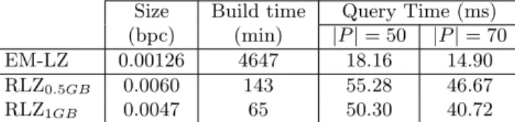
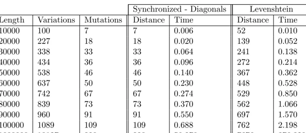
In larger collections we first compared the EM-LZscan and RLZ con-struction methods, observing that using RLZ the index can be built more than 50 times faster, with little impact on the size index. Table 4.1 repro-duces the results in one of those collections. Then we compared the parallel version of RLZ against the sequential one. The results of one of those ex-periments is reproduced here in Table 4.2. Finally, we tested our index in a 2.4TB collection2 that took about 12 hours to index and in which exact occurrences of query patterns were found in less than 100ms .

2

The DNA collections used to test scalability were supposed to be “x versions of human chromosome y”. However, due to a regrettable mistake in Paper II this is not the case. The misuse of an external tool to generate the data resulted on genetic variants being greedily applied to the first genome with no overlapping variants, generating a col-lection with some genomes containing most of the variants, and many identical genomes. As a consequence, although those experiments prove that the method can handle large collections, the resulting times and spaces do not reflect the behavior on a proper collec-tion of genomes. In the next chapter this is handled properly, so e.g. Table 5.1 gives a better idea of the behavior of CHICO on real data.

(36)

26

Size Build time Query Time (ms) (bpc) (min) |P|= 50 |P|= 70 EM-LZ 0.00126 4647 18.16 14.90 RLZ0.5GB 0.0060 143 55.28 46.67

RLZ1GB 0.0047 65 50.30 40.72

Table 4.1: Different parsing algorithms to index collection CHR21, a 90GB

syn-thetic collection made of DNA. The first row shows the results for EM-LZ, which computes the LZ77 greedy parsing. The next rows show the results for the RLZ parsing using prefixes of size 500MB and 1GB. The size of the index is expressed in bytes per char, the building times are expressed in minutes, and the query times are expressed in milliseconds. Query times were computed as an average of 1000 query patterns randomly extracted from the collection.

Size Build time (min) Query Time (ms) (bpc) LZ Parsing Others P=50 P=70 RLZ1GB 0.00656 308 51 225.43 178.47

PRLZ1GB 0.00658 22 55 224.04 181.21

Table 4.2: Results using RLZ and PRLZ to parse CHR14, a 201 GB synthetic

collection made of DNA. Query times were computed as an average of 1000 query patterns randomly extracted from the collection.

(37)

Chapter 5 Pan-Genome Read Alignment to

Improve Variation Calling

An important motivation that we have discussed in previous chapters isread alignment, where short NGS reads are mapped to a (much larger) genomic reference. In essence, to do read alignment is to solve approximate pattern matching.

Among the many applications of read alignment [57], here we focus on variation calling, the process of characterizing an individual’s genome by finding how it differs from a reference. The standard approach is to obtain a set of reads from the donor, to map them to a single reference genome using a read aligner, and analyzing the read pile-up to infer the variants that occur in the donor’s genome.

However, our current knowledge about the human genome is pan-genomic [19]: after the first human genome was sequenced, the cost of sequencing has decreased dramatically, and today many projects are curating huge genomic databases.

In this chapter we present the contribution of Paper III, a new frame-work for variant calling with short-read data utilizing a pan-genomic ref-erence. As an intermediate result we provide a fully scalable pan-genome read aligner based on the index of Chapter 4.

5.1 Pan-genome indexing

As DNA repositories keep growing the termpan-genome is being used more frequently [66, 87, 88, 19] – even getting media coverage [81, 73] – although not always with the same meaning. A recent attempt for a broad definition states that apan-genome is any collection of genomic sequences to be

(38)

28 5 Pan-Genomic Variation Calling

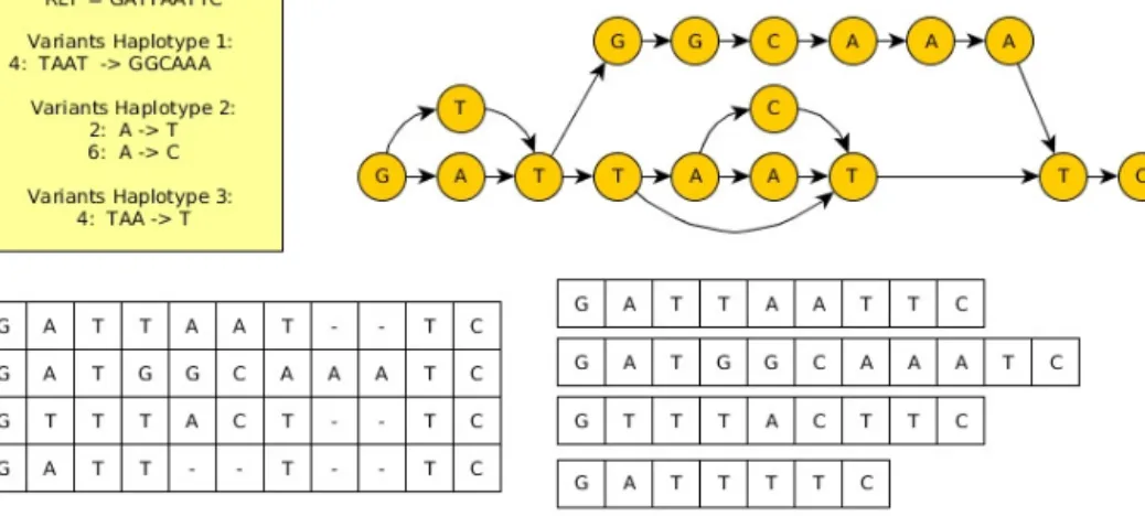
Figure 5.1: Four different representations of a pan-genome that corresponds to the same set of individuals. Top left: a reference sequence plus a set of variants to specify the other individuals. Top right: a (directed acyclic) graph representation. Bottom left: a multiple sequence alignment representation, Bottom right: a set of sequences representations.

lyzed jointly or to be used as a reference [19]. Once we adopt this general definition for pan-genomic reference, we are left with two closely related questions: how to represent a pan-genomic reference, and how to index it. Previous efforts can roughly be categorized into three classes: one can consider (i) a graph representing a reference and variations from it, (ii) a set of reference sequences, or (iii) a modified reference sequence. See Paper III for a review on these approaches [86, 84, 46, 21, 24, 71, 29, 23, 64].

The simple class (ii) model, a set of sequences, has been actively studied from a computer science perspective, achieving good results in terms of time and space efficiency using scalable methods. Unfortunately, unlike classes (i) and (iii), it has not been tested for enhancing variation calling. Here we aim to fill this gap. We do it by adopting a multiple sequence alignment representation of the pan-genome. On the one hand, it is easily transformed into a set of sequences and vice versa. On the other hand, similarly to class (i) and (iii), the multiple sequence alignment has enough structure to make it an attractive choice for a reference.

(39)

5.2 Pan-genomic references to improve variant calling 29

5.2 Pan-genomic references to improve variant

calling

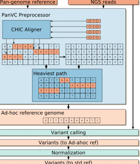
In this section we present our framework for variation calling using read alignment to a pan-genomic reference. First we give an overview, and then we dwell on the relevant details. Figure 5.2 illustrates our scheme.

Our approach represents the pan-genome reference as a multiple se-quence alignment (Figure 5.1 bottom left). We index the underlying set of sequences in order to align the reads to the pan-genome. After aligning all the reads to the pan-genome we perform a read pileup on the multiple sequence alignment of reference genomes. The multiple sequence alignment representation of the pan-genome lets us extract a linear ad hoc reference easily. Such a linear ad hoc reference represents a possible recombination of the genomic sequences present in the pan-genome that is closer to the donor than a generic reference sequence. The ad hoc reference is then fed to any standard read alignment and variation detection workflow. Finally, we need to normalize our variants: after the previous step, the variants are expressed using the ad hoc reference instead of the standard one. The normalization step projects the variants back to the standard reference.

In the following sections we provide a detailed description of each com-ponent of our workflow.

5.2.1 CHIC aligner

We developed CHIC aligner, an extended version of the previous chapter’s index. Using it we can perform read alignment to the set of sequences that makes the pan-genome. Recall that CHICO indexes a set of sequences using a recent data structure called hybrid index [29]. The hybrid index uses the Lempel-Ziv compression algorithm to factor out repetitions in the sequences and builds a sequence containing only the non-repetitive content. This sequence has been called kernel sequence, because to solve the pattern matching problem in the whole sequence, it is enough to solve it in the kernel sequence. In addition to the kernel string and its index, CHIC aligner also stores the phrase boundaries, and some auxiliary information. This is necessary to project the coordinates of the alignments from the kernel string to the original sequences. Different algorithms from the Lempel-Ziv algorithms can be used to construct the index, leading to different trade-offs. Among them we chose Relative Lempel-Ziv (RLZ) [56] because of its many virtues for the pan-genome scenario: it offers a very fast construction algorithm with moderate memory requirement and little compromise in the size of the index. Furthermore it can be easily run in parallel. Once the

(40)

Figure 5.2: Schematic view of our PanVC workflow for variation calling, including a conceptual example. The pan-genomic reference comprises the sequences GATTATTC, GATGGCAAATC, GTTTACTTC and GATTTTC, represented as a multiple sequence alignment. The set of reads from the donor individual is GTTT, TTAA, AAAT and AATC. CHIC aligner is used to find the best alignment of each read. In the example, all the alignments are exact matches starting in the first base of the third sequence, the third base of the first sequence, the seventh base of the second sequence, and on the eight base of the second sequence. After all the reads are aligned, the score matrix is computed by incrementing the values of each position where a read aligns. With those values, the heaviest path algorithm extracts a recombination that takes those bases with the highest scores. This is the ad hoc genome which is then used as a reference for variant calling using GATK. Finally the variants are normalized so that they are using the standard reference instead of the ad hoc reference.

(41)

5.2 Pan-genomic references to improve variant calling 31 kernel sequence is built, CHIC aligner indexes it with a standard read aligner, such as Bowtie2 or BWA.

A feature that CHIC aligner has in common with some previous indexes for pan-genomes is that during indexing time, a context sizeM is given as a parameter. This sets an upper bound for the read length that can be aligned. In all our experiment we useM = 120.

CHIC aligner interface is compatible with other reads aligners: the input is a multi-fasta file with the input genomes and the alignments are output in the SAM format [59]. Our index offer two main reporting modes for the alignments: The first one looks for the best alignment in the kernel string and only its projection back to the original input is reported. The second one also looks only for the best match in the kernel string. Then its projection to the input is reported, and also all possible repetitions of such alignment are reported as well. Those can be combined with Bowtie2 (or BWA) reporting options, and instead of looking for the best match in the kernel string, it is possible to report all occurrences, or the bestkones, where k is a user-defined parameter. In our experiments we report only the best alignment, as it is expected that many repetitions occur in the pan-genomic context.

5.2.2 Pan-genome representation

As discussed in Section 5.1, we represent the pan-genome as a multiple sequence alignment and we index the underlying sequence using CHIC aligner. To transform one representation into the other and to be able to map coordinates we store bitmaps to indicate the positions where the gaps occur. Consider our running example of a multiple alignment

GATTAAT--TC GATGGCAAATC GTTTACT--TC GATT--T--TC

We may encode the positions of the gaps by four bitvectors:

11111110011 11111111111 11111110011 11110010011

Let these bitvectors beB1, B2, B3,and B4. We extract the four sequences

(42)

and selectqueries [48, 16, 68]: rank1(Bk, i) =j tells the number of 1s in

Bk[1..i] andselect1(Bk, j) =itells the position of thej-th 1 inBk. Then,

for Bk[i] = 1, rank1(Bk, i) = j maps a character in column i of row k in

the multiple sequence alignment to its positionj in the k-th sequence, and

select1(Bk, j) =idoes the reverse mapping, i.e. the one we need to map

a occurrence position of a read to add the sum in the coverage matrix. These bitvectors with rank and select support taken+o(n) bits of space for a multiple alignment of total size n [48, 16, 68]. Moreover, since the bitvectors have long runs of 1s (and possibly 0s), they can be compressed efficiently while still supporting fast rank and select queries [79, 72].

5.2.3 Heaviest path extraction

After aligning all the reads to the multiple sequence alignment, we extract a recombined (virtual) genome favoring the positions where most reads were aligned. To do so we propose a generic approach to extract such a heaviest path on a multiple sequence alignment. We define a score matrix S that has the same dimensions as the multiple sequence alignment representation of the pan-genome. All the values of the score matrix are initially set to 0. We use CHIC aligner to find the best alignment for each donor’s read. Then we process the output as follows. For each alignment of length m that starts at positionj in the genomeiof the pan-genome, we increment the scores in S[i][j], S[i][j+ 1]. . . S[i][j+m−1]. When all the reads have been processed we have recorded in S that the areas with highest scores are those where more reads were aligned.

Then we construct the ad hoc reference as follows: we traverse the score matrix column wise, and for each column we look for the element with the highest score. Then, we take the nucleotide that is in the same position in the multiple sequence alignment and append it to the ad hoc reference. This procedure can be interpreted as a heaviest path in a graph: each cell (i, j) of the matrix represents a node, and for each node (i, j) there are N outgoing edges to nodes (i+ 1, k), k _{∈ {}1, . . . , N_}. We add an extra node A with N outgoing edges to the nodes (1, k), and another node B withN ingoing edges from nodes (L, k). Then the ad hoc reference is the sequence spelled by the heaviest path from A to B. The underlying idea of this procedure is to model structural recombinations among the indexed sequences.

A valid concern is that the resulting path might contain too many alter-nations between sequences in order to maximize the weight. To address this issue we propose an algorithm to extract the heaviest path, constrained to have a limited number of jumps between sequences (see Paper III,

Algorithms and Data Structures for Sequence Analysis in the Pan-Genomic Era