Generating Headlines with Recurrent Neural Networks

(1)

Chalmers University of Technology University of Gothenburg

Generating Headlines with Recurrent

Neural Networks

Bachelor of Science Thesis in Computer Science and Engineering

ALEX EVERT, JACOB GENANDER, NICKLAS LALLO,

RICKARD LANTZ, FILIP NILSSON

(2)

(3)

Bachelor of Science Thesis

Generating Headlines with Recurrent Neural Networks

ALEX EVERT

JACOB GENANDER

NICKLAS LALLO

RICKARD LANTZ

FILIP NILSSON

Department of Computer Science and Engineering

CHALMERS UNIVERSITY OF TECHNOLOGY

University of Gothenburg

(4)

(5)

Generating Headlines with Recurrent Neural Networks ALEX EVERT JACOB GENANDER NICKLAS LALLO RICKARD LANTZ FILIP NILSSON

Examiner: NIKLAS BROBERG

Department of Computer Science and Engineering Chalmers University of Technology

University of Gothenburg SE-412 96 Göteborg Sweden

Telephone: +46 (0)31-772 1000

The Author grants to Chalmers University of Technology and University of Gothenburg the non-exclusive right to publish the Work electronically and in a non-commercial purpose make it accessible on the Internet.

The Author warrants that he/she is the author to the Work, and warrants that the Work does not contain text, pictures or other material that violates copyright law. The Author shall, when transferring the rights of the Work to a third party (for example a publisher or a company), acknowledge the third party about this agreement. If the Author has signed a copyright agreement with a third party regarding the Work, the Author warrants hereby that he/she has obtained any necessary permission from this third party to let Chalmers University of Technology and University of Gothenburg store the Work electronically and make it accessible on the Internet.

Department of Computer Science and Engineering Göteborg 2016

(6)

Acknowledgments

First and foremost, we would like to thank our supervisor Mikael Kågebäck for giving us insightful feedback and input during the project. We would also like to thank him and the machine learning group (LAB) for letting us use their compute server. Finally, we would like to give acknowledgment to the people from the department for technical language, who gave us useful suggestions on the thesis.

(7)

Generating Headlines with Recurrent Neural Networks

A

LEX

E

VERT

JACOB

GENANDER

NICKLAS

LALLO

RICKARD

LANTZ

FILIP

NILSSON

Department of Computer Science and Engineering, Chalmers University of Technology

University of Gothenburg Bachelor of Science Thesis

Abstract

This report describes the implementation and evaluation of two natural language models using the machine learning technique deep learning. More specifically, two different models describing recurrent artificial neural networks (RNNs) were imple-mented, capable of generating news article headlines. One model focused on the generation of random (unconditioned) headlines, and the other one on the gener-ation of headlines based (conditioned) on a given news article. Both models were then trained and evaluated on a data set of approximately 500,000 pairs of news

articles and their corresponding headlines. The task of summarizing large bodies of text into smaller ones, while maintaining the key points of the original text, has many applications. Quickly and automatically obtaining condensed versions of for example medical journals, scientific papers, and news articles can be of great value for the users of such content. The unconditioned model, implemented using a multi-layer RNN consisting of LSTM cells, was able to produce headlines of mod-erate plausibility, a majority being syntactically correct. The conditioned model was implemented using two RNNs consisting of GRU cells in an encoder-decoder-network with an attention mechanism, allowing the encoder-decoder-network to learn what words to focus on during headlining. Although the model managed to identify important keywords in the articles, it seldomly managed to produce meaningful sentences with them. We conclude that the techniques and models described in this report could be used to generate plausible news headlines. However, for the purpose of generating conditioned headlines, we think that additional modifications are needed to obtain satisfying results.

(8)

(9)

Sammanfattning

Denna rapport beskriver implementationen och utvärderingen av två språkmodeller med maskininlärningstekniken deep learning. Två olika modeller av återkopplande

artificiella neuronnät (RNNs) implementerades, båda kapabla att generera rubriker till tidningsartiklar. En av modellerna fokuserade på generering av slumpmässiga (obetingade) rubriker, och den andra på generering av rubriker baserade (betingade) på en given nyhetsartikel. Båda modellerna tränades på ett dataset med ca. 500,000

par av artiklar och deras tillhörande rubriker. Att sammanfatta stora textstycken till mindre sådana, där huvudpoängerna i originalet bevaras, har många tillämpningar. Att snabbt och automatiskt kunna få fram sammanfattade versioner av exempelvis medicinska journaler, vetenskapliga papper, och nyhetsartiklar kan vara av stort värde för dess användare. Den obetingade modellen implementerades med ett RNN organiserat i flera lager. Cellerna i nätverken var av LSTM-typ. Detta nätverk pro-ducerade måttligt trovärdiga rubriker. Den betingade modellen implementerades med två stycken RNNs beståendes av GRU-celler ordnade i ett encoder-decoder

-nätverk med attention. Detta ger nätverket möjlighet att lära sig vilka ord som

är viktigast vid rubriksättningen. Modellen lyckades visserligen identifiera viktiga nyckelord i artiklarna, men hade svårt att sätta ihop dessa i vettiga meningar. Vår slutsats är att teknikerna som beskrivs i denna rapport skulle kunna användas till att generera trovärdiga nyhetsrubriker. Trots detta tror vi att det krävs ytterli-gare modifikationer för att kunna generera trovärdiga betingade rubriker på ett tillfredsställande sätt.

(10)

(11)

Glossary

n-gram Word frequency based language model. 3 ANN Artificial Neural Network. 1, 9, 13

DMN Dynamic Memory Network. 40

dropcost Method for reducing cost variation in sequential output. III, 3, 21, 25,

37, 41

GRU Gated Recurrent Unit. vii, 12, 25

LSTM Long Short-Term Memory. v, vii, xv, 11, 12, 24, 29 NLP Natural Language Processing. 1, 41

NNLM Neural Network Language Model. 14

RNN Recurrent Neural Network. v, vii, xv, 2, 10, 11, 14–16, 40 RNNenc The basic encoder-decoder model. 14

RNNsearch Encoder-decoder with an attention mechanism. xv, 3, 14, 16, 17, 24,

40

RNNsearch* Encoder-decoder with an attention but with sentences as inputs. 3,

17, 40

(12)

(13)

List of Figures

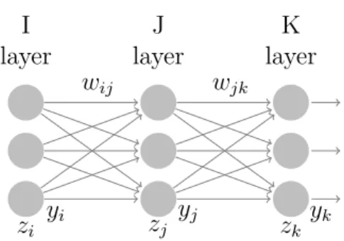
2.1 Three layer feed-forward neural network. Each layer labeled by its receptive index variable with inputs z, outputs y and weightsw. . . . 8

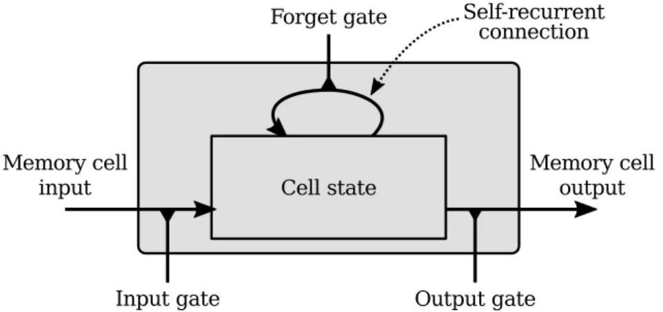
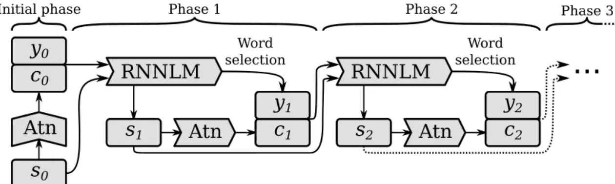
2.2 Schematic drawing of an LSTM cell with its input, output, gates and cell state. Notice that the cell state has a recurrent connection. . . . 12 3.1 Schematic description of the data flow, RNNLM refers to the

un-conditioned language model and Atn to the attention model. The

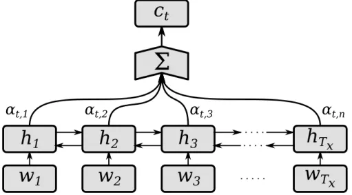
phases are the steps of the model and the word selection is done from the softmax output during generation and the target sequence during training. . . 15 3.2 Data flow for computing the output of the decoding RNN in RNNsearch.

The summation is the scalar product used to calculate the expected annotation ct. . . 16

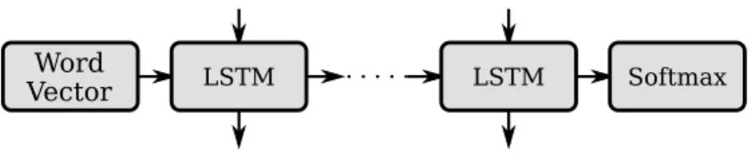
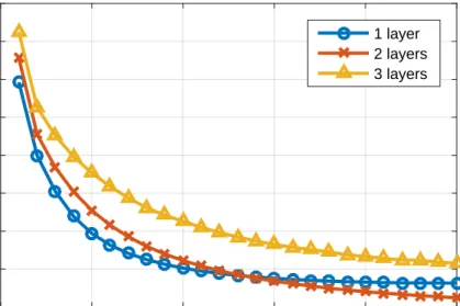
5.1 Final architecture of the unconditioned language model. A word vec-tor propagates through several LSTM layers and finally through the softmax function, giving a distribution of what the next word might be. The vertical arrows indicates how the LSTM cells’ states move between time steps. . . 24 6.1 Cost on training set during the optimization process. Three different

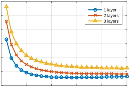
models were evaluated with roughly the same number of parameters, differing only in number of layers and layer size. . . 30 6.2 Cost on validation set during the optimization process. Three models

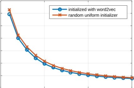
with different number of layers were compared against each other. All three models had 50% dropout added to avoid overfitting. . . 31 6.3 Cost on training set when using different ways of initiating the word

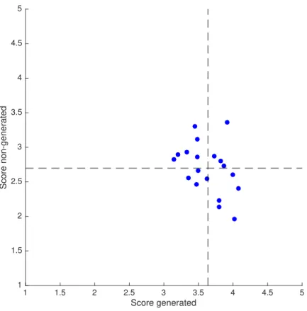
vectors in a 1-layer model. Pretrained word2vec [1] vectors were com-pared against a random uniform initializer between -0.1 and 0.1 . . . 32 6.4 Average score for generated and non-generated headlines in each test,

indicated by the dots. Total average score for generated and non-generated headlines are indicated by the vertical and horizontal dashed lines respectively. This shows how the average score for generated headlines is higher than for non-generated, which is undesired when trying to generating plausible headlines. . . 34 6.5 The perplexity for the conditioned model on two different sets of

(18)

(19)

List of Tables

5.1 Machine specifications . . . 25

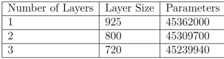
6.1 Model configurations and number of parameters . . . 29

6.2 Validation and test perplexity at epoch with lowest cost . . . 31

(20)

(21)

1

Introduction

Creating a computer program that generates syntactically and semantically correct text is a difficult task. One approach is to, given some previous words in a sentence, estimate the conditional probability of each word in the language being the next in the sentence. It is then possible to choose one that seems likely, and repeat the pro-cess with the newly extended sentence. For example, the sentence ”The cat crossed the...” would seem to be more likely to end with ”street” or ”bridge” than ”sea” or ”introduce”. The question is what the probability is for each of these words, or any word in the language at hand for that matter, to be the next word in the sen-tence? Modeling relationships of this kind within a language is in the field of natural language processing (NLP) often referred to as language modeling. Traditionally, language models have been constructed using eithern-gram models [2] or rule-based

models [3] [4] [5]. A problem with n-gram models is that they only take the n−1

previous words into consideration when generating the next. This means that the end of a sentence may not be directly related to the beginning. Moreover, as each permutation of then−1 words yields a probability, both memory and computational

requirements increase exponentially with respect to n. A problem with rule-based

models is that they require hand-crafted word type tagging [5], which takes time and would have to be done explicitly for each modeled language.

When solving the language modeling problem with artificial neural networks (ANN), less time is spent on the complex task of describinghowto detect patterns and

mean-ing in the text. Instead, a model describmean-ing a network of interconnected artificial neurons is designed, whose structure and properties are chosen as to facilitate the network’s ability to learn the desired characteristics of the text by example. For

instance, if the network is presented with example sentences where ”The cat crossed the” is frequently followed by ”bridge”, then the internal state of the network should be automatically adjusted towards outputting a higher probability for ”bridge” as the next word in that particular sequence. Such a task requires a lot less engineering [6], as the network will take care of most of the “thinking” itself. In addition, a well designed model requires few or no modifications, before it can be trained and used for similar tasks, e.g. to generate headlines for news articles or for medical health notes. The network described is used in a type of machine learning called deep learning,

which has risen in popularity lately. It is a method in which multiple neural net-works are stacked in layers, and doing so enables the network to learn compositional representations of, for example, words [6]. This can be intuitively understood as having each consecutive layer learn more abstract representations of the words, by

(22)

1. Introduction

analyzing the simpler representations received from the layers before it. By making it possible for the neurons to loop back information to earlier stages of the sequence, we get something similar to memory. These kinds of neural networks where in-formation can persist is known as recurrent neural networks (RNNs), and is the implementation used throughout this project. In the context of RNNs, the notion of deepness in a network often refers to the number of steps in the sequence. The ability to remember things makes these networks especially interesting in language modeling, as we try to generate sentences based on previous words the network has seen. Hence, using RNNs as a language model seems to be appropriate, as words towards the end of a sentence often depend on previous words.

Furthermore, looking at natural language processing, many approaches to sentence-decomposition uses a tree-like structure [3], where words represented by the leaves of a tree, are grouped together to form a sentence at the root. The widespread use of such methods to model language [4] [7] [5] [8], also suggests that a layered archi-tecture, although not tree-structured, might be a suitable approach for constructing our network models.

The generation of text using the previously mentioned methods has many appli-cations. A statistical model can be used for tasks where the next word in a sequence is to be predicted, for example auto-completion in smartphone keyboards, whereas a conditioned model could be used for abstractive summarization tasks. The task of abstractive summarization aims at providing summaries of text, without extract-ing whole sentences from it [9]. This poses the problem of havextract-ing to generate new sentences, which incorporate the most essential information from the original text. Some possible use-cases for such summarizations are medical journals, scientific pa-pers, and news articles. In these cases, an automated approach might be preferable because of its speed, or due to a reduction of manual labor.

1.1 Purpose

In this paper we implement two artificial neural networks, examining the advan-tages of using memory-capable cells and multiple network layers, to try and solve two natural language tasks involving text generation:

1. Generation of random news headlines

2. Generation of news headlines, based on some input text (e.g. part of an article) Regarding the first goal, the headlines should be random in the sense that they are not based on some input text, but have the style of news headlines in general (e.g. formulated as statements or questions and not too long).

In the second goal, each headline will be conditioned on a news article. This will be done using an attention model so that the network can choose, on its own, which parts of the article that are most relevant for the headline.

(23)

1. Introduction

1.2 Scope

The project will only involve training the networks on English text, since adding an additional language would make the task more complex. Learning multiple lan-guages, the training time of the networks would probably be longer as well. Further, the networks will only be trained to generate headlines for articles, not for books or other written media. We aim to train the networks to recognize the specific style of headlines. To mix this style with e.g. book titles could lead to headlines that do not seem natural to find among articles.

The networks approximate an unknown conditional distribution that changes dra-matically over time, i.e. the style of newspaper articles from the 19th century may be very different from those written in the past 10 years. Articles stemming from different sources may also be very different in style. This could potentially be a problem when measuring how good the networks generate an appropriate headline for a given article. Therefore, we will narrow down the time span for publication dates of the articles.

1.3 Related Work

Early attempts to approximate the propability of a sequence w of words, P(w),

relied on n-grams, that is, sequences of n consecutive words. The assumption is

that languages obey the n−1:th order Markov property, i.e. that words in a text

depend only on their index and then−1 words before them. Using this assumption,

one could instead aim to approximate the probability of a wordwt occuring at time

step t, given all the previous words in the sequence, by calculating the probability

of a word wt occuring at time step t, given only the n −1 previous words. That

is, P(wt|wt1−1) = P(wt|wtt−−n1+1), where the right hand side could be found using a

simple frequency count. This gave

P(wt|wtt−−n1+1)≈

C(wt)

P

wi∈VC(wi)

whereC(wj) is the number of occurrences of the wordwj after the sequencewtt−−1n+1in

the corpus. The subscript and superscript inwt_t₋−_n1₊₁denote the first and last element

respectively in the sequencewthat are taken into concideration. These models have

problems with scaling, considering that whenn grows, the frequencies become very

low. The assumption that languages have this Markov property is also trivially false for small n. Extending the models to cluster words [10] did however manage

to achieve respectable perplexities on large corpuses using only 3-gram models.

1.4 Contributions

In this thesis we propose the objective modification technique dropcost as described in 4.3. We also propose a variation of RNNsearch, RNNsearch*, detailed in 3.4.

(24)

1. Introduction

This variation has, to the best of our knowledge, never been implemented. Both of these contributions needs further study before any conclusions can be drawn.

1.5 Structure

The report begins with a background consisting of several chapters explaining the principles behind artificial neural networks, language models, and different training concepts. This is followed by a chapter describing the methods used, and details about the implementation. After that, there is a chapter describing the results from the project and finally a chapter discussing these results.

(25)

2

Artificial Neural Networks

There are many concepts related to the field of machine learning. In the following sections, we will describe the essential parts of the techniques used in this project. The explanations are not exhaustive, but should rather give the reader an under-standing of how they work and what their purposes are.

2.1 Feed-Forward Neural Networks

Artificial neural networks model complex functions by learning from experience. No code is needed to tell the network explicitly what to do. Instead, it is a process of tuning certain parameters and looking at the result as data is input.

The fundamental building block of any neural network is the neuron. The neu-ron takes a number of inputs, processes them and outputs a result that decides its activation. What the output will be depends on the neuron’s state. In its sim-plest form, the state consists only of a number of weights, one for each input. The weighted inputs are added together and put into an activation function. An acti-vation function is a function that gives a smooth transition between two distinct values, like 0 and 1. The two extremes can be seen as two modes, on or off, for the neuron. In many cases, a bias is also added together with the weighted inputs. The bias can be thought of as a number telling us how easy it is to activate a certain neuron. If a bias is included, it is also part of the state.

To construct a network, we order several neurons in interconnected layers, where the activation from one layer is the input to the next. Layers have different names depending on where in the order they are placed. The first layer is the input layer, then come the hidden layers and lastly the output layer. The input layer can take a number of input values simultaneously, which is referred to as feeding the network. In our case, this will be a vector representation of a word where each element will be treated as a separate input value.

A more mathematical definition of the input of a neuron and its activation can be written as follows. Let zk = X j wjkxj+bk (2.1)

(26)

2. Artificial Neural Networks

be the input of a neuronk (other than in the input layer), where the sum is over all

neuronsj in the previous layer, wjk the weight from j tok, xj the output of j and

bk the bias term ofk. The activation of the neuron k can then be written as:

g(zk) = 1

1 + e−zk (2.2)

2.1.1 The Softmax Function and Sampled Softmax

The final layer in the network should output a probability distribution over the dif-ferent classes. In our models, the classes are words and the distribution shows the probabilities for the next word. This distribution is calculated using a special activa-tion funcactiva-tion called the softmax funcactiva-tion. It is a multidimensional generalizaactiva-tion of the logistic function (see Equation 2.2) and very common for classification problems. Letσ(z)j denote the softmax function, wherez is the input and j denotes a specific

class for which the softmax value is to be calculated.

σ(z)j =

ezj

PK

k=1ezk

, for all k = 1,2, ..., K (2.3) zj is in our case the input to the neuron in the final layer, corresponding to

word-numberj in the vocabulary. The sum in the denominator is over all words k in the

vocabulary, which consequently normalizes the sum of all softmax values in the final layer to 1.

As a consequence of using large vocabularies, the training complexity increases [11], in part due to the amount of parameters in the network. Using neural networks to translate text from one language to another, it has been shown that decreasing the size of the vocabulary also makes the translation performance decrease rapidly[11], i.e. the quality of the output probability distribution degrades. A possible remedy to this problem is to use a technique called sampled softmax.

Sampled softmax uses only a subset of all words in the vocabulary to calculate how the probabilities of words should be updated in each iteration during training. Since only a fixed amount of word probabilities are adjusted, the computational complexity is kept constant with respect to the vocabulary size [11].

Using sampled softmax, since only a fixed amount of classes are adjusted, regardless of vocabulary size, the computational complexity is kept constant with respect to the vocabulary size.

2.2 Training

The parameters of the network has to be tuned to produce the desired output. This is done like a classical optimization problem. Since we know what the desired outputs are, we can compare these with the actual output. The difference is formulated as a cost function and we minimize this by changing the weights and biases. Training a network this way is known as supervised learning [6].

(27)

2.2.1 Negative Log Likelihood

To get a measure of how well our model made its predictions, we are going to use the negative log likelihood for the target words.

cost =− 1 N N X i=1 lnptargeti (2.4)

Instead of just seeing how far from 100% the probability was for a specific word, this more sophisticated function will improve the learning process when used together with the softmax function [12]. One can get an intuitive feel for the function by understanding that all output word probabilities will be between 0 and 1 and that the cost will decrease as the probabilities for certain words go closer to 1. Notice that we take the average of several predictions since the training is done in batches.

2.2.2 Stochastic Gradient Descent

During training, the task is to minimize the cost of the output as a function of the parameters, namely the weights and biases. An analytic way of finding the minima of a function is to differentiate it and look for its extreme points. But since the system is going to be overdetermined, this has to be done numerically. In our case, a method known as gradient descent will be used.

The graph of the cost function can be thought of as a multidimensional landscape, where each parameter corresponds to a dimension. At each iteration of the opti-mization process, a step is taken in the opposite direction of the gradient. The gradient is a vector of the partial derivatives of the cost function, indicating in what direction the function is increasing the most. Therefore, we want to move in the opposite direction of the gradient. How long we keep going before calculating the gradient anew is decided by the learning rate. Increasing the learning rate might make the learning process faster, but there is also the risk of diverging from a local minimum. However, this may in some cases be desired, since a local minimum not necessarily is the global minimum. After a fixed number of steps or when the results do not seem to improve, the learning process is over.

Calculating the cost over the whole data set each training iteration is computa-tionally heavy [13]. To speed up the process, the data will instead be divided into several smaller batches. The network is then trained on one batch at a time. This updates the gradient more quickly but with less accuracy, since only a portion of the data set is considered. Doing so will most likely not generate the shortest path to a local minimum, but has the advantage of stochasticity. As the updates are somewhat off compared to the gradient of the whole data set, it is possible to escape local minima [14]. Using gradient descent with smaller batches (sometimes called mini-batches) of the data set is known as stochastic gradient descent (SGD).

(28)

2.2.3 Adam Optimizer

The Adam optimizer (Adaptive Moment Estimation) [15] is a gradient decent opti-mization algorithm. Its goal is to speed up the training while still being accurate. Since some parameters of the input data change more drastically and frequently than others from input to input, the value of a single fixed learning rate may be suitable for some parameters but not to others. Being close to the minimum in one dimension of parameter space would suggest that slow moves towards it are suitable (as explained in subsection 2.2.2), while on the contrary, some other parameters may be farther away from their respective minimum, suggesting that a faster learn-ing rate would be suitable for them. Instead of uslearn-ing a slearn-ingle learnlearn-ing rate for all parameters or predetermined ones for each of them, the Adam optimizer computes individual adaptive learning rates for each of them. It incorporates both the ex-ponentially moving average of the objectives’ gradient and the squared gradient in order to estimate moments (mean and uncentered variance) of the gradient. The effect of the moments can be thought of as applying momentum to the gradient, preserving velocity longer when moving downhill in parameter space and reducing velocity quicker when moving uphill.

2.2.4 Backpropagation

Calculating the partial derivatives needed for the gradient can get quite complex because of all the different variables the partial derivatives depend on. This is especially a problem in large networks with multiple layers, as it would require cal-culating the output of the network as many times as there are weights and biases in it (using the definition of the derivative)[12]. One method to solve this is the back-propagation algorithm. This algorithm makes use of previously calculated values in order to calculate the new ones. It is based on the chain rule, and here follows an example, which shows how to calculate the partial derivatives needed to update the weights of the network.

J layer I layer layerK zi yi wij zj yj wjk zk yk

Figure 2.1: Three layer feed-forward neural network. Each layer labeled by its

(29)

Let’s say we have a feed-forward ANN as in Figure 2.1 [16] with layers I,J and K,

where K is the output layer of the network. Let wjk be the weight from neuron j

in layer J to neuron k in layer K, yj the output of j and zk =P j

wjk ·yj the input

of k. Also, let _∂yk∂E =rk be the partial derivative of the errorE, with respect to the

output yk (i.e. the partial derivative of the error function). In our case, the error

function is defined by the cost function in Equation 2.4

In order to update the weightwjk, we need to calculate the partial derivative _∂wjk∂E .

We can start by noting that ∂E ∂zk =

∂E ∂yk ·

dyk

dzk. The partial derivative of the output yk

with respect to the inputzk is the derivative of the activation functionf(zk) (w.r.t.

zk), so ∂E ∂zk = ∂E ∂yk ·dyk dzk =rk·f0(zk)

This is why the activation function must be differentiable. Here we made use ofrk,

which is done only for the output layer K. When propagating the error backwards

further into the network, we would like to use the equivalent value of the partial derivative of the error E with respect to the output y in any layer other than K.

Since the forward-propagated signal branches onto several neurons, we sum over these neurons. For the next layer,J, we obtain

∂E ∂yj =X k ∂E ∂zk ∂zk ∂yj As∂zk

∂yj is the change in input ofkwith respect to the output ofj, it can be substituted

by the corresponding weight,wjk, and we obtain

∂E ∂yj =X k ∂E ∂yk wjk (2.5)

Now, we can continue by writing ∂E ∂wjk as ∂E ∂wjk = ∂E ∂zk · ∂zk ∂wjk Notice how ∂zk

∂wjk = yj. This might seem a bit puzzling, but can be motivated by

asking the question ”how does the input of neuronk,zk, change with respect to the

weightwjk?”. Since zk =P j

wjk·yj, the change is yj, and we write

∂E ∂wjk

= ∂E

∂zk

·yj (2.6)

Equation 2.6 shows how to calculate the desired partial derivative specifically for a weightwjk from layerJ toK. The resulting value can be used to update the weight,

as shown in Equation 2.7

wjknew =wjkold−η

∂E ∂wjk

(30)

where wjknew and wjkold refer to the updated and old value of wjk respectively, η

is the learning rate and the minus sign before it indicates that we update in the opposite direction of the gradient. This is done for all weightswjk. Now we continue

backwards in the network by repeating the process. We can calculate the partial derivative of the error with respect to the weights in the next layer,wij, by

∂E ∂wij = ∂E ∂zj · ∂zj ∂wij = ∂E ∂zj ·yi

similarly to what we did in 2.6. For the purpose of explaining the algorithm, it suffices to say that ∂E

∂zj can be found by using the previously calculated value in 2.5.

For the same reason, biases of the neurons were not taken into consideration.

2.2.5 The Vanishing Gradient Problem

As explained in subsection 2.2.4, calculating gradients of weights near the input layer requires calculating gradients of the weights between subsequent layers. This comes with a problem, namely the vanishing gradient problem. It becomes espe-cially evident for deep [12] and recurrent networks [17], the latter being discussed in section 2.3.

Each layer in the network works as a function of its input. The output layer of the network can therefor be considered to be a function of some other functions, corresponding to the previous layers. Using a logistic function as activation func-tion, the derivative of a neuron’s output (w.r.t. to its input) lies in the range (0,1₄]

[12]. When many of these small terms are multiplied, as when calculating the gradi-ent in a deep or recurrgradi-ent network, the product becomes smaller and smaller for each multiplication. In effect, the gradient of the error w.r.t. the weights near the input layer can become impractically small when training [17] - the gradients vanish. As the gradient is calculated using weights as well, the opposite may happen for large enough values of the weights, making the gradient explode [12].

One solution to the vanishing gradient problem is to use a so called constant error carousel with gates, suggested by [17]. The carousel ensures that the gradient of the

activation remains constant, while the gates ensure that only relevant information is corrected for during the backpropagation.

2.3 Recurrent Neural Networks

Recurrent neural networks (RNN) is a type of neural networks that are used for mod-eling time sequences, such as words in a sentence. By remembering their previous state,st−1, they can make better predictions of what comes at timet. The problem

with simply looping back information is that the network quickly forgets what it has just seen . Longer time sequences will thus be harder to model. A solution is to introduce a number of gates which control what the network should remember and forget. This helps with the vanishing gradient problem discussed in 2.2.5, and to

(31)

this end, the Long Short-Term Memory cell was invented [17]. The output of both gated and plain RNNs will, for inputxt, be referred to as RNN(st−1, xt).

2.3.1 Long Short-Term Memory

Long Short-Term Memory, LSTM, is a special network architecture that has the ability to remember certain values for longer time, while discarding others imme-diately. This is accomplished by using four so called gates, which are trained to control the flow of information within the cell, sometimes also called the hidden unit [17]. The cell has a memory called the cell state that contains the information from previous steps, see Figure 2.2. The gates incorporate parts of the old state when calculating the new. Each iteration part of the state is either retrieved, over-written or kept unchanged for the future. We can describe the LSTM cell and its state asCl

t, wheret is the time step, and l is the layer that it resides in.

The cell takes two inputs. The first is its own cell state from the previous time step, and the second is the output from the previous layer at the current time step, concatenated with its own output from the previous time step. In the case where the cell is in the first layer, the input is the word vector itself. It will then use these inputs to calculate the output as well as to update its own state for the next time step. In our case, each time step will be used for calculating one word vector. The forget gate layer is there to decide what to keep in the cell state and what to forget. It uses a sigmoid layer, i.e. a layer with the logistic function as activation function. We will call the output from the forget gate f. Let’s also use b for bias

vectors,xt for the cell’s input, and W for weight matrices inside gates.

f =σ(Wf ·[xt,ht−1] +bf) (2.8)

The input gate layer uses both a tanh layer to calculate new inputs into the cell state and a filtering sigmoid layer to decide what to save. Like a sigmoid layer, the tanh layer is correspondingly a layer that uses tanh as activation function. Let’s call the output of the tanh layerg and that of the sigmoid layer i, we now get:

i=σ(Wi·[xt,ht−1] +bi) (2.9) g= tanh(Wg·[xt,ht−1] +bg) (2.10) Cl_t =f Cl_t₋₁+ig (2.11)

where denotes element-wise multiplication. After calculating the new cell state,

there is a final output layer to decide what to output from the cell state. It uses a tanh neural net layer on the cell state as well as a sigmoid layer on the input to filter the information from the tanh layer. The output hl_t can then be calculated.

The filtered output, o, from the sigmoid layer is obtained by:

o=σ(Wo·[xt,ht−1] +bo) (2.12) hl_t =otanh(Cl_t) (2.13)

(32)

Figure 2.2: Schematic drawing of an LSTM cell with its input, output, gates and

cell state. Notice that the cell state has a recurrent connection.

2.3.2 Gated Recurrent Unit

Another type of cell or hidden unit that can be used in networks is the Gated Recurrent Unit (GRU), introduced as a simpler version of the LSTM [18]. While the LSTM cell has four gates to control the flow of information, this model instead only has two gates; a reset gate as well as an update gate. Despite being far less computationally heavy than the LSTM cell, empirical studies have shown it to perform comparably [19].

2.4 Deep Neural Networks

A minimal network would consist of only one input layer and one output layer. Using multiple hidden layers in between are referred to as a deep neural network, hence the name deep learning. Having multiple layers, the network may gain performance. However, there seems to be no precise explanation of when this is true, i.e. no precise relationship between performance and the number of layers. Testing multiple setups of networks is therefore common practice.

(33)

3

Language Models

The two main goals of the project are to create a program that generates random headlines and another that generates headlines based on the beginning of a news ar-ticle. To this end, two different language models are used, namely an unconditioned language model for the first goal and a conditioned one for the second goal. The following subsections will describe each model and their corresponding approaches to solving the problems.

3.1 Word Embeddings

Unlike images and sound, words in a language do not carry any information, but instead act merely as tokens. Thus, a space of objects represented as a sequence of words have no natural metric, and the dimensionality of the space will grow expo-nentially with the length of the sequence. Trying to approximate some probability mass function on such a space is notoriously hard, simply because the probability for any one element will be close to zero. This is known as the curse of dimensionality

[20].

To remedy this problem, [20] introduced the concept of distributed representations of words, or word embeddings, where words are mapped to elements in Rm.

Typ-ically m ∈ _N is significantly smaller than the vocabulary in the language, and the

vectors are tuned to make some problem well-conditioned. In the contexts of ANN, it is common to represent words asw∈ {0,1}|V| _with_|_w_|_{= 1 and to insert a simple} linear embedding layer that multiplieswwithW ∈_R|V|×m. The weights_W are then

trained together with the network. The vectorwwill be refered to as asparse word representation.

W can be initialized in many ways, either randomly using some sensible distribution

or by first training an ANN to minimize some problem based on the distributional hypothesis in lingustics introduced by [21] and using these weights in a more

inter-esting problem. Notable such pretraining models have been constructed by [22] and [23].

3.2 The Unconditioned Language Model

The starting point of language models is assigning probabilities to sequences of words. Once this is achieved, one can use this distribution to either draw sentences

(34)

3. Language Models

or judge existing sentences. Ifw is a sequence of words, wi the i:th element of that

sequence and wj_i a sub-sequence from i to j the probabilities can be computed by

using the chain rule on the prefixes in the sequence, i.e.

P(w) =Y

t

P(wt|w1t−1)

To estimate the conditional probabilities P(wt|w1t−1) as a multinomial distribution

over the vocabulary V, an RNN is trained to minimize the negative log likelihood

of a softmax output.

The standard model introduced by [20] used a feed-forward neural network and is often referred to as NNLM. This model was later extended by [22] to use an RNN instead. In its most basic version, the model is given by the following equations

st =f(Uwt+Wst−1) yt =σ(Vst)

whereU ∈_R|V|×m _{is a word embedding,} _W _∈

Rm×m simply some trainable weights, σ is the softmax function, V ∈ _Rm×|V| _{a linear mapping and} _f _{some activation} function. Of course, this simple activation RNN can be replaced by an arbitrary recurrent cell which output can than be mapped onto the vocabulary and given to the softmax function.

3.3 The Conditioned Language Model

Many tasks can not be solved by a simple language model and require the generated sentence to be conditioned on some input sequence. Even though RNNs are well suited for processing sequential data, they have problems taking sequences as inputs since they require the input dimension to be known and fixed. In statistical ma-chine translation, this problem has been successfully solved by different variations of encoder-decoder networks [18][24].

These models train two RNNs together — one that encodes an input sequence to a fixed sized vector and one that decodes that vector to a target sequence — using standard gradient based optimization through the whole system. These ba-sic models will be referred to as RNNenc. Later these models have been extended using an attention mechanism introduced by [25] where instead of trying to encode the original sequence in a single vector, the encoder gives a list of vectors relevant to different parts of the original sequence. The decoder is trained to decide which vectors are relevant for the next word given the currently generated sequence. This model will be referred to as RNNsearch.

3.3.1 The Basic Encoder-Decoder Model

In RNNenc, the context c representing the input sequence x1, . . . , xTx is typically

(35)

3. Language Models

either forward as in [18] or backwards as in [24].

The conditioned probability that the wordw ∈ V should appear next in the

gener-ated sequencey1, . . . , yt is then modeled as

P(yt =w|y1t−1, xTx1 )≈σ V RNN st−1, " yt−1 c #!! ·w0 whereV ∈_Rm×|V| _, _s

t−1 is the internal state of the RNN after the model has

gener-ated distributions for the words y1, . . . , yt−1 and w0 is a sparse word representation

as described in 3.1. Note that the context vectorchas been concatenated to the

in-put. Further,s0 is 0∈Rmandy0 is a wordg not appearing in the target vocabulary.

This is essentially the same as the unconditioned model only that the input vec-tors have been extended to not only carry information about the word,yi, but also

a condensed version , c , of the input sequence. During training the target words yi are not picked from the output but instead read from the target sequence, when

generating sequences the output distribution is used to pick the next word to give to the model.

Sometimes when discussing implementation details, the block of the weight matrices that deals with the concatenated context is factored out, as is done in [25].

3.3.2 Encoder-Decoder with Attention

s

₀

y

₀

c

₀

Atn

RNNLM

Atn

c

1

s

1

y

1

c

2

s

2

y

2

Atn

RNNLM

Word selection

Initial phase Phase 1 Phase 2

Word

selection

...

Phase 3

Figure 3.1: Schematic description of the data flow,RNNLM refers to the

unconditioned language model andAtn to the attention model. The phases are the

steps of the model and the word selection is done from the softmax output during generation and the target sequence during training.

The encoder in RNNSearch instead produces Tx annotation vectors, hi, consisting

of the concatenation of the internal states of one RNN run forward on the input sequence up to word i and one run backwards to the same word. Alignments eij

(36)

3. Language Models

approximate the likelihood of the word yj aligning to annotationhi, i.e

P(yj aligns to hj)≈αji

αj =σ(ei)

eij =a(si−1, hj)

wherea(si, hj) is some trained alignment model. A context cj is then computed as

the expected annotation

cj =αj ·h

and used in a decoder entirely analogous with the decoder in RNNenc. An overview of the data flow is given in Figure 3.1 where Atn refers to the attention model

described here. The data flow of the attention model can be viewed in Figure 3.2.

w

₁

w

₂

w

₃

w

_Tx

h

₁

h

₂

h

₃

h

_Tx

α

t,1

α

t,2

α

t,3

α

t,n

Σ

c

_t

Figure 3.2: Data flow for computing the output of the decoding RNN in

RNNsearch. The summation is the scalar product used to calculate the expected annotation ct.

3.4 A Variation on the Conditioned Language Model

Conditioning the model as in 3.3 introduces problems with scaling [26][27], partly because the increased amount of attention contexts and time steps. It might also be because of the underlying assumption of RNNsearch that generated words align to one specific word.

When setting a title on a text it might thus be useful to try to reduce both the number of time steps and attention contexts by considering the text not as a se-quence of words but instead as a sese-quence of sentences. This also helps motivate the plausibility of the assumption, i.e it’s more plausible that words in the title aligns to particular article sentences rather than particular article words.

(37)

3. Language Models

Sentences can be effectivly represented as vectors [28] and when that has been done, those vectors can be fed to RNNsearch with no modifications. This is, to the best of our knowledge, a novel model which we introduce and call RNNsearch*. Further, the whole model can still be trained by gradient based optimization algorithms via backpropagation.

(38)

(39)

4

Training Concepts

There are many concepts in the context of training ANNs, both regarding the train-ing data and the elements of the network. All of these concepts affect the final performance and the following subsections will explain the key ideas behind those used in this project.

4.1 Hyperparameters

Some parameters cannot be learned, but have to be set manually. These so called hyperparameters are mainly related to the specific learning algorithm and structure of the network. Tuning these is done not only to improve training results, but also to generalize the model so it can make better predictions on cases it has not seen before. Learning the training set too closely is known as “overfitting”and choosing the right hyperparameters can prevent this. Following is a more detailed explanation of the different hyperparameters and their effect on the model.

4.1.1 Layer Size

When choosing the number of hidden units in each layer, it is important to choose a size that is big enough [29]. Larger than optimal values will not hurt performance, but it will increase the time it takes to train the network. A larger network also means more parameters available for tuning which can lead to overfitting [12].

4.1.2 Training/Validation Data Ratio

To acquire good results, it is essential that the network has high-quality and ex-tensive data to learn from. We also need data which can be used to validate the network’s performance. One hyperparameter is then how we should distribute our data set between training and evaluation. It is important to have a validation set that is disjoint from the training set, as it gives an indication of the networks ability to generalize. If the validation was to be done on the training set, it would have been difficult to tell whether the network was overfitting or not.

4.1.3 Number of Epochs

One epoch is one run through the data set and running several epochs could yield better results. Still, we do not want the model to learn the data set too closely. The number of epochs will also affect how long the training takes.

(40)

4. Training Concepts

4.1.4 Learning Rate

As discussed in subsection 2.2.2, it is possible to increase the learning rate to make more radical changes to the variables each optimization step. A low learning rate will not improve the cost as much as we want, but a too big step might never converge to a minimum. One way of choosing a fitting learning rate is to look at the graph of the cost function, and see whether it decreases satisfactorily each time step. It is also common to decrease the learning rate as the training progresses. In that case, when to begin the decrease and by how much are also parameters to decide.

4.1.5 Word Dimensionality

Another hyperparameter is the input size of the network, i.e. the dimensionality of the word embeddings. If pre-trained word vectors are used, this hyperparameter is equivalent to their dimensionality.

4.2 Regularization

The process of reducing overfitting while maintaining the size of the network is called regularization and the following paragraphs will explain the two main regularization techniques used in this project.

4.2.1 Dropout

Dropout is a technique described in [30] that aims to prevent overfitting. By remov-ing some neurons and their connections within the network durremov-ing trainremov-ing (with a probabilityp), it can be seen as training random subsets of the whole network. When

the training has ended, no dropout is applied, meaning that all neurons and con-nections are present. The weights may then be scaled by the probability p, which

makes the output of a neuron equal to the expected output during training with dropout. The result is a network consisting of many sub-networks that have been trained differently from each other. This has been shown to increase performance on various machine learning tasks. While capable of increasing the effectiveness of the network, dropout also increases the training time, since only a fraction of the whole network is trained each iteration. The dropout probability pis a hyperparameter.

4.2.2 Early Stopping

One way to detect overfitting is to compare the performance of the network on the training set with that of the validation set. In the beginning of the training process, the network should improve on both sets. However, after some training, the performance on the validation set may become worse, while that of the training set keeps on becoming better. This could indicate that the network is learning the training set too specifically and cannot generalize to the validation set. To prevent this, we can simply stop training when the performance of the two sets begins to diverge. However, it might be difficult to determine when to stop, as divergence

(41)

4. Training Concepts

could be temporary. One way to circumvent this is to save the network at different checkpoints during training and then pick the one which has best performance on the validation set.

4.3 Dropcost

When optimizing sequence-generating models using the average negative log like-lihood (see subsection 2.2.1) of the sequence, there’s a risk that the average cost can be lowered by diverging from the target sequence in some systematic manner. To penalize this we propose a variation of the regularization technique dropword

introduced by [31]. We will refer to this variation asdropcost. Whiledropword hides

input words from the model trying to penalize over dependence on part of the in-put, dropcost instead waives costs in the output sequence, benefiting models with

low variation in the cost for the generated outputs. The expected fraction of the words in a target sequence with wavered costs during training will be referred to as the dropcost factor.

4.4 Mini-Batch Size

Choosing to train on one word pair each iteration would adjust the parameters towards better predicting the next word, given the first word in particular. On the other hand, training on the whole data set each iteration would adjust the parameters towards better predicting the next word for all words in the set at once. The first approach has the advantage of stochasticity, meaning that the parameters can escape local minima more easily, while the latter approach speeds up the process by enabling parallel calculations of several words. A commonly used technique is to train on a so called mini-batch each iteration, which contains a subset of the whole data set. Choosing the size of the mini-batch is a balance between efficiency and effectiveness.

(42)

(43)

5

Method

This section describes how the proposed models were implemented, what tools were used for doing so and how the validation of the outcome was conducted.

5.1 Data Sets

A set of over 540,000 articles with corresponding headlines was sampled for training and validation data in both models. The data set was produced by Congle Zhang and Daniel S. Weld, by querying the Bing news search engine for news articles based on the titles in RSS news seeds. This was done using daily news seeds from multiple newspapers between January 1 to February 22, 2013 [32].

5.1.1 Preprocessing the Data Sets

The data set was pre-processed before tokenization to reduce the amount of unique tokens generated from it. Also, some incomplete entries (titles without articles etc.) were removed. All text went through the following processing before being tokenized and used in the models:

lower-casing All text was converted to lower-case.

number-normalization All digits were replaced by zeros.

5.2 The Unconditioned Model

This section describes the implementation of the language model from section 3.2.

5.2.1 Data processing

Only titles from the data set were used, and tokenized using a tokenizer from the Natural Language Toolkit (NLTK). This tokenizer provides multiple tools such as separating shortened word combinations, for example ”couldn’t” becomes two to-kens: ”could” and ”n’t”. A vocabulary was then created, containing only tokens occurring more than 5 times. Less frequently occurring tokens were replaced with the ”unknown-token”, ”_UNK”.

(44)

5. Method

5.2.2 Implementation

Figure 5.1 shows the final architecture of the unconditioned language model. A word vector is put through one or several LSTM layers and the output from the last one will be used as input to the softmax function. The softmax function gives a probability distribution over the dictionary for what the next word might be. When generating the headlines, the program will choose a word from this distribution and then use it as input at the next time step. Also, at each time step the LSTM cells’ states are updated.

Figure 5.1: Final architecture of the unconditioned language model. A word

vector propagates through several LSTM layers and finally through the softmax function, giving a distribution of what the next word might be. The vertical

arrows indicates how the LSTM cells’ states move between time steps. The different layers are connected with weights, as described in 2.1. These are the parameters that get tuned during the optimization step together with the word em-beddings. It is worth noting that the model trains on several sequences at once and calculates the average cost. To accelerate the training process, the word embeddings are initialized with pretrained word2vec vectors [1]. These have been trained on part of Google News’ data set.

5.3 The Conditioned Model

This section describes the implementation of the RNNsearch language model from subsection 3.3.2.

5.3.1 Data processing

In the conditioned model, all articles and titles were first converted into tokens using a simple white-space tokenizer. Two different vocabularies were created, consisting of the 40,000 most common words1 found in the articles and titles respectively. Each

article-title-pair was then truncated to a fixed length of 200 tokens for articles and 50 tokens for titles.

5.3.2 Implementation

The conditional language model is implemented using the seq2seq-library from Ten-sorflow The model is an implementation of an encoder-decoder network described

(45)

5. Method

in subsection 3.3.1 with the addition of attention as described in subsection 3.3.2. Just like in [25], the implementation uses a single feed-forward tanh layer as the alignment model.

When training the network, the article-title-pairs were fed through the encoder-decoder network in batches of 16 or 32 pairs, depending on the other hyper pa-rameters’ impact on RAM usage. The network was implemented with GRU-cells, ranging from 512 to 1024 cells in 2 or 4 layers. For each batch, a loss was calculated, and network parameters (vector representations and annotations) adjusted using the Adam [15] optimizer. Every 100 batches, the perplexity was noted and a checkpoint of the model was saved.

5.3.3 Dropcost

To evaluate dropcost two networks identical to the conditioned network with 1024 cells and 2 layers but with dropcost factors of 0.15 and 0.30 respectively were trained.

Then 100 articles from the validation set where sampled and headlines generated by all three networks. The 10 articles on which the network without dropcost was judged to have performed the best were selected and the networks performance on these 10 articles where then qualitatively compared.

5.4 Environment

The models described in this section have been implemented using the machine learning framework TensorFlow [33] by Google. Data processing and other book-keeping tasks have been implemented in Python 2. Bash scripts were used to manage the execution of simultaneous jobs on the compute server.

The training and evaluation of the models were done either on a GPU-equipped workstation (when not limited by the RAM of the GPU), or on Chalmers’ Machine Learning group’s Compute server. Specifications for these machines can be found in Table 5.1. Notable is that the NVIDIA GTX 970 GPU can be described as a more consumer oriented product, both regarding price and performance, while the NVIDIA Titan X is oriented more towards enthusiasts and scientific calculations.

Table 5.1: Machine specifications

Specification Workstation Compute server

CPU Intel i7-4790K (8·4 GHz) Intel i7-5930k (12·3.5 GHz)

GPU NVIDIA GTX 970 (4 GB) 4x NVIDIA Titan X (12 GB) RAM 16 GB DDR3 32 GB DDR4

(46)

5. Method

5.5 Optimizing Hyperparameters

There are many parameters that can be tuned manually to increase the performance of the models. Getting all the parameters right can take a lot of time and because of that we are going to focus on the ones that clearly increase performance and are easiest to tune. The process can best be described as trial and error, where a couple of models are trained with different values and their results compared. However, there are some heuristics to follow.

The size of a network can affect its performance, where a larger network can learn more sophisticated patterns than smaller ones. A large network also has higher probability of overfitting and therefore often has to be compensated with increased dropout. One way to see if the model is overfitting is to compare the cost for the training and validation set. These should both be decreasing when training and not differ too much from each other.

Besides network size and dropout ratio, the most important parameter to tune is the learning rate. Typical values for our case is in the range of less than 1 and greater than 10−6 _{[29]. When trying different learning rates it is often more constructive}

to test different multiples of the original learning rate than just increasing it with some decimal value. The graph of the cost function can be inspected to see whether the training progresses as desired or not. A too steep cost function often indicates a too big learning rate and a cost function that looks more linear often means that the learning rate is too small.

When it comes to mini-batch size and number of training epochs, these parame-ters mainly affect the program’s running time and will not be crucial to the end results. Together with network size, they will however decide how long it takes to go through the data. Therefore, they are still important since time is limited.

5.6 Evaluation

In order to evaluate the performance of the models implemented for the project aims, the following two measures were considered.

5.6.1 Perplexity

Perplexity is a measurement used to evaluate how well a model predicts a sample. Many research papers use this measurement, so it is useful if we want to compare our work with that done by others in similar projects. In our case we calculate the per-word perplexity with the formula e cost

words.

5.6.2 Turing-like Test

To further evaluate the the first goal (generating random news headlines), a Turing-like test was used. In 1950, Alan Turing devised a test for validating how well

(47)

5. Method

machines can imitate humans, by letting a human try to determine if a conversa-tion is held with a computer or another human [34]. The test used in this project consisted of 100 random generated headlines and 100 random non-generated head-lines from the training set, presented as 20 smaller tests with five generated and five non-generated headlines in each. A smaller test would be randomly chosen and presented to the participant, who were then asked to, for each headline, indicate how certain they were that a given headline was generated or non-generated, using an integer scale from 1 (”non-generated”) to 5 (”generated”). This way, the plausi-bility of the headlines could be evaluated in finer detail than when having to choose between ”generated” or ”non-generated” only. The answer values for each headline would then be summed and averaged. An average value of 3 would indicate that a headline was as plausible as unplausible. The best result achievable for a generated headline would be 1, where as the worst would be 5, with respect to the project aims. There were no restrictions made on who could participate in the test or how many smaller tests could be taken by the same person. This was justified by not showing the correct answers in the end of the test. Each of the smaller tests consisted of the same headlines every time it was presented, but in random order, as this may contribute to less bias when answering.

(48)

(49)

6

Results

After implementing and training the models, they could be evaluated using the techniques described in Evaluation. The following sections describe how the different models ultimately performed. In order to give an indication of their performance, some examples of generated headlines are shown as well.

6.1 The Unconditioned Language Model

The unconditioned model was trained on an Nvidia GTX 970 graphics card. The biggest model able to fit on one of theses cards had about 45,3 million parameters. This value represents all adjustable weights and biases: LSTM cell states, word em-beddings, weights between the different layers in the model and the neurons’ biases. Three separate models were trained with roughly the maximum number of param-eters, differing only in number of layers and layer size. The different configurations can be seen in Table 6.1.

Table 6.1: Model configurations and number of parameters

Number of Layers Layer Size Parameters 1 925 45362000 2 800 45309700 3 720 45239940

To reduce memory requirements the Adam optimizer was used [15]. Each model was trained for 25 epochs with a batch size of 50, and the learning rate was kept constant at 0.002. 10% of the data set was used for evaluation. Using the method described in subsection 5.2.1, the vocabulary ended up with a size of 33300 words.

Generating Headlines with Recurrent Neural Networks

Generating Headlines with Recurrent

Neural Networks

ALEX EVERT, JACOB GENANDER, NICKLAS LALLO,

RICKARD LANTZ, FILIP NILSSON

Bachelor of Science Thesis

Generating Headlines with Recurrent Neural Networks

ALEX EVERT

JACOB GENANDER

NICKLAS LALLO

RICKARD LANTZ

FILIP NILSSON

Department of Computer Science and Engineering

CHALMERS UNIVERSITY OF TECHNOLOGY

University of Gothenburg

Acknowledgments

Generating Headlines with Recurrent Neural Networks

A

E

JACOB

GENANDER

NICKLAS

LALLO

RICKARD

LANTZ

FILIP

NILSSON

Abstract

Sammanfattning

Glossary

Contents

List of Figures

List of Tables

1

Introduction

1.1

Purpose

1.2

Scope

1.3

Related Work

1.4

Contributions

1.5

Structure

2

Artificial Neural Networks

2.1

Feed-Forward Neural Networks

2.1.1

The Softmax Function and Sampled Softmax

2.2

Training

2.2.1

Negative Log Likelihood

2.2.2

Stochastic Gradient Descent

2.2.3

Adam Optimizer

2.2.4

Backpropagation

2.2.5

The Vanishing Gradient Problem

2.3

Recurrent Neural Networks

2.3.1

Long Short-Term Memory

2.3.2

Gated Recurrent Unit

2.4

Deep Neural Networks

3

Language Models

3.1

Word Embeddings

3.2

The Unconditioned Language Model

3.3

The Conditioned Language Model

3.3.1