(will be inserted by the editor)
The Time-Dependent Orienteering Problem with
Time Windows: A Fast Ant Colony System
C´edric Verbeeck, Pieter Vansteenwegen, El-Houssaine Aghezzaf
the date of receipt and acceptance should be inserted later
Abstract This paper proposes a fast ant colony system based solution method to solve realistic instances of the time-dependent orienteering problem with time windows within a few seconds of computation time. Orienteering problems occur in logistic situations where an optimal combination of locations needs to be selected and the routing between these selected locations needs to be optimized. For the time-dependent problem, the travel time between two locations depends on the departure time at the first location. The main contribution of this paper is the design of a fast and effective algorithm for this problem. Numerous experiments on realistic benchmark instances with varying size confirm the state-of-the-art performance and practical relevance of the algorithm.
1 Introduction
The orienteering problem (OP) is defined on a graph in which the vertices repre-sent geographical locations where a reward can be collected. An arc in the graph represents a connection between two vertices and has a certain travel time. The goal of the OP is to determine which subset of vertices to visit and in which order so that the total collected reward is maximized and a given maximum total travel time is not exceeded. In addition, a feasible OP solution should start and end at a predetermined vertex. The OP integrates the knapsack problem (KP) and the travelling salesperson problem (TSP). In contrast to the TSP, not all vertices can be visited in an OP due to the limited travel time. However, determining the shortest path for visiting the selected vertices might decrease the total travel time and help to visit extra vertices.
The OP has many interesting applications in defence, tourism and logistics. For example, a military application of the OP considers Unmanned Aerial Vehicle
Ghent University, Industrial Engineering Systems and Product Design, Technologiepark 903, 9052 Zwijnaarde - Belgium, Tel.: +32 9 264 54 95, Fax.:+32 9 264 58 47
E-mail: [email protected], [email protected] ·KU Leuven, Leuven Mobility Research Center, 3001 Leuven - Belgium E-mail: [email protected]
(UAV) mission planning to collect intelligence information about different loca-tions in the area of operaloca-tions (see for example (Royset and Reber, 2009; Mufalli et al, 2012; Evers et al, 2012)). The aim of these missions is to acquire as much information as possible during the flight, while the length of the flight is limited by the available fuel capacity of the UAV. Another application of the OP is personal-ized tourist trip planning. In this case, each vertex is a point of interest (POI) and the reward of a POI indicates the personal interest that the tourist attaches to it. In this problem, a tourist wants to visit several different sightseeing locations, for each of which the tourist has a different preference level. The length of the tourist tour is restricted by the total time the tourist can spend on sightseeing. Research on this problem and similar applications was presented in (Vansteenwe-gen and Van Oudheusden, 2007; Vansteenwe(Vansteenwe-gen et al, 2011b; Souffriau et al, 2008; Schilde et al, 2009; Wang et al, 2008). Finally, OPs are used in logistic planning tools where each vertex represents a customer and the reward reflects the profit margin achieved by visiting this customer. The aim is to select the combination of customers and sequence that maximizes the total profit (Tsiligirides, 1984; Golden et al, 1987; Kantor and Rosenwein, 1992). For a longer list of practical and real-life applications of the OP and its variants, we refer to the survey by Vansteenwegen et al (2011a).
In optimisation problems such as the OP, the travel time required to traverse a link between two vertices can be considered either independent or time-dependent. If the time to traverse a link is not dependent on the hour of the day (time-independent orienteering problem or the regular OP), it is considered to be static and it is represented by a single value. If, on the other hand, this travel time is time-dependent, this problem is called the time-dependent orienteering problem (TD-OP). Then the travel time depends on the hour of the day the link is taken and it can no longer be modelled by a single value. In this case, this is modelled as a travel time function representing the travel time in function of the hour of the day. As thoroughly discussed in (Verbeeck et al, 2014), the time-dependent problem formulation allows to tackle congestion related issues in routing problems and multi-modal applications for logistic or tourist trip planners.
Furthermore, in the problem we consider, each vertex has a time window (open-ing time and clos(open-ing time) and a service time. The addition of time windows to the time-dependent orienteering problem makes the problem more realistic since both tourist attractions and customers also have opening hours in real-life situations. It is therefore an obvious step in the direction of modelling and solving realis-tic routing problems (Aghezzaf et al, 2012). On the other hand, by incorporating time windows, the resulting waiting times, which postpone the start of a service and thus the departure time, directly affect the travel times in a time-dependent problem context. This makes the problem more difficult than the TD-OP without time windows. For example, departing earlier at a vertex, to avoid congestion, might turn out to be less useful if you can not serve the subsequent vertex at the scheduled arrival time because of the opening time.
This paper makes several contributions to the literature. Firstly, the TD-OPTW is introduced and mathematically modelled. Secondly, an ant colony op-timization algorithm is proven to be successful in solving realistic test problems for the TD-OPTW. Thirdly, a set of problem instances based on a large and real road network are made available together with an efficient pre-processing method. This method also allows a fast execution of any solution method for the OP or
related problems such as the TSP and the vehicle routing problem (VRP) with time-dependent travel times. In general, this paper tries to show how a vehicle routing problem with time-dependent disturbance can be tackled in a practical way. The pre-processing method and solution method presented in this paper are ready to be incorporated in vehicle route planners. Finally, the impact of account-ing or not for time-dependent travel times for the OPTW is investigated. It shows the importance of taking into account time-dependent travel times and leads to some managerial insights.
Following a literature review in Section 2, the TD-OPTW is further described in Section 3. Then, the pre-processing procedure and solution method are proposed in Section 4. Afterwards, the creation of the datasets based on a realistic network is discussed in Section 5. The solution methods are experimentally evaluated in Section 6. Section 7 concludes this paper and discusses possible future work.
2 Literature Review
The name of the orienteering problem derives from the sport game of orienteering (Tsiligirides, 1984; Chao et al, 1996). In this game, individual competitors start at a specified control point and try to maximize their reward by visiting checkpoints and returning to the control point within a given time frame. Each checkpoint has a known reward and the objective is to maximize the total collected reward. A survey on the OP and its extensions can be found in Vansteenwegen et al (2011a) and Gunawan et al (2016).
The time-dependent variant of the OP is relatively new and has, to the best of our knowledge, only been studied in (Fomin and Lingas, 2002; Abbaspour and Samadzadegan, 2011; Garcia et al, 2013; Li et al, 2010; Li, 2011; Gavalas et al, 2014, 2015). Fomin and Lingas (2002) were the first authors to mention the TD-OP and state that it is NP-hard because the TD-OP is NP-hard. However, they do not develop an algorithm for the TD-OP that can be used in practical situations. Abbaspour and Samadzadegan (2011) introduce a solution procedure for the TD-OPTW based on two adaptive genetic algorithms and multi-modal shortest path finding modules. They are able to solve multi-modal routing problems in the city of Tehran, although no absolute performance measure (gap) was reported. Li et al (2010) propose a mixed integer programming model of the TD-OP combined with an optimal pre-node labelling algorithm based on the idea of network planning and dynamic programming. However, this algorithm is not tested on benchmark instances and therefore no performance metrics are proposed. The same conclu-sion holds for Li (2011) where a mixed integer programming model is proposed and an optimal dynamic labelling algorithm is designed for the time-dependent team orienteering problem (TD-TOP). Garcia et al (2013) develop aniterated local search(ILS) heuristic for the time-dependent team orienteering problem with time windows (TD-TOPTW) which allows them to illustrate, based on a case study in the city of San Sebastian, that obtaining near-optimal routes in a few seconds is feasible. However, only a special case of time-dependency is considered, which is the result of using public transport in a city environment. For example, when a traveller arrives at a bus stop before the bus arrives he needs to wait. Therefore the travel time between two vertices consists of both the waiting time and the driving time and depends on the departing time at the start vertex. They exploit
the fixed frequency of bus services to come up with an efficient solution technique. The most recent work is from Gavalas et al (2014) and Gavalas et al (2015). The authors propose several cluster-based heuristics for the TD-TOP applied to tourist trip planning. Unlike Garcia et al (2013), they do not make the assumption of pe-riodic service schedules. The algorithms were tested on datasets compiled from the metropolitan area of Athens.
Existing solution methods for the related time-dependent vehicle routing prob-lem (TD-VRP) (Ichoua et al, 2003; Haghani and Jung, 2005; Lecluyse et al, 2009; Van Woensel et al, 2008; Kok et al, 2012) and the time-dependent vehicle rout-ing problem with time windows (TD-VRPTW) (Potvin et al, 2006; Chen et al, 2006; Donati et al, 2008; Kritzinger et al, 2011; Hashimoto et al, 2008; Soler et al, 2009; Balseiro et al, 2011) provide inspiration on how to efficiently deal with time-dependency and time windows. The work of Lecluyse et al (2009) even incorporates stochastic time-dependent travel times. Soler et al (2009) transform TD-VRPTW into an Asymmetric Capacitated Vehicle Routing Problem in order to solve it with a state-of-the-art exact and heuristic solution method. The algorithms that have been developed for the TD-VRP(TW) include tabu search (Ichoua et al, 2003; Van Woensel et al, 2008; Lecluyse et al, 2009), a genetic algorithm (Haghani and Jung, 2005), a heuristic combining route construction and route improvement (Potvin et al, 2006; Chen et al, 2006), two ant colony system approaches (Donati et al, 2008; Balseiro et al, 2011), a variable neighborhood search (Kritzinger et al, 2011) and iterated local search (Hashimoto et al, 2008). Kok et al (2012) use a time-dependent shortest path algorithm together with a restricted dynamic pro-gramming heuristic to solve real-life TD-VRP test instances. In (Verbeeck et al, 2014) we developed a solution procedure for the TD-OP and tested it on modified OP instances. However, these instances were based on a simplistic speed-model adopted from the TD-VRP literature. This algorithm was tested on modified OP instances that consist of a complete graph where all arcs between vertices needed to be assigned to a road category which defined their travel time profile. In this paper we extend the TD-OP solution procedure to incorporate time windows and we add the swap and replace local search procedures. More importantly, we ver-ify that realistic problem instances that originate from a large road network with available travel time profile measurements can be solved effectively and efficiently by our heuristic solution procedure.
3 Problem description
In this section, the time-dependent orienteering problem is described and modelled as a Mixed Integer Programming (MIP) formulation.
Formally, the TD-OPTW can be described by defining a set Vc = {1, ..., v} of vertices. In this set vertex 1 represents the start depot and vertex v the end depot. We assume there is an arc (i,j) between alliandjinVc. Associated with each vertexi∈Vcis a non-negative reward ri. This reward is earned by visiting the vertex for a duration ofsi time units between its opening timeoi and closing timeci+si. The vertex can not be visited at any other moment in time. Note also that the time window is defined for the start of the service and not the end. The reward of the start and end depot is equal to 0.
We assume that a day is divided inκtime slots. Furthermore, let us assume that
tstandtstrepresent the moment at which time slottstarts and ends respectively. Subsequently, based on these time slots and their corresponding travel times for each arc (tti,j,tst), the linear travel time coefficients for each arcµi,j,t andνi,j,t can be calculated as follows:
µi,j,t=
tti,j,tst−tti,j,tst tst−tst
(1a)
νi,j,t=tti,j,tst−µi,j,t∗tst (1b) These linear regression coefficients allow the travel time fromitoj, when departing at timewi,j,tin time slott(tst< wi,j,t< tst), to be calculated as follows:
tti,j,wi,j,t =µi,j,t·wi,j,t+νi,j,t (2) During this process the linear piecewise travel times are guaranteed to be FIFO if
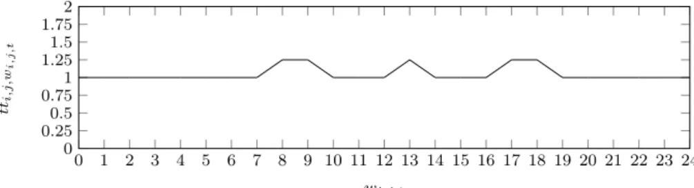
|µi,j,t|is smaller than or equal to 1.5. A visual example of a piecewise linear travel time for an arci, j can be seen in Figure 1. In this example, there are 24 timeslots (κ) with a length of 1 hour. For t= 7,µi,j,7 equals 0.25 andνi,j,7 equals −0.75 which results intti,j,wi,j,7= 0.25∗wi,j,7−0.75.
0 1 2 3 4 5 6 7 8 9 10 11 12 13 14 15 16 17 18 19 20 21 22 23 24 0 0.25 0.5 0.75 1 1.125.5 1.75 2 wi,j,t tti,j ,w i,j ,t
Fig. 1 Example of a piecewise linear travel time on an arci, jwithκ= 24
The decision variables and other parameters used in the MIP model are listed below:
Decision variables
xi,j,t=1 if a vehicle traverses the arc (i, j) with a departure time in time slott, 0 otherwise
wi,j,t=departure time at vertex i when travelling from i to j in time slot t, 0 otherwise
Parameters
µi,j,t: slope coefficient of the linear time-dependent travel time as defined in Equa-tion (1a)
νi,j,t: intercept coefficient of the linear time-dependent travel time as defined in Equation (1b)
tst: start of time slot t
κ: number of time slots
ri: reward of vertexi oi: opening time of vertexi ci: closing time of vertexi si: service time of vertexi tmax: time budget
Max v−1 X i=2 v X j=2 κ X t=1 ri·xi,j,t (3a) v X j=2 x1,j,1= v−1 X i=1 κ X t=1 xi,v,t= 1 (3b) v−1 X i=1 κ X t=1 xi,h,t= v X j=2 κ X t=1 xh,j,t≤1 ∀h= 2, ..., v−1 (3c)
xi,j,t·tsi,j,t≤wi,j,t i= 1, ..., v−1, j= 2, ...v,∀t (3d) wi,j,t≤xi,j,t·tsi,j,t i= 1, ..., v−1, j= 2, ...v,∀t (3e)
v−1 X i=1 κ X t=1
[wi,h,t+µi,h,t·wi,h,t+ (νi,h,t+sh)·xi,h,t]≤ v X j=2 κ X t=1 wh,j,t ∀h= 2, ..., v−1 (3f) v−1 X i=1 κ X t=1
[wi,v,t+µi,v,t·wi,v,t+νi,v,t·xi,v,t]≤tmax (3g)
v−1 X i=1 κ X t=1 (oh+sh)·xi,h,t≤ v X j=2 κ X t=1 wh,j,t ∀h= 2, ..., v−1 (3h) v X i=2 κ X t=1 wh,i,t≤ v−1 X i=1 κ X t=1 (ch+sh)·xi,h,t ∀h= 2, ..., v−1 (3i) w1,i,1= 0 ∀i= 1, ..., v (3j) xi,j,t∈(0,1) i, j= 1, ..., v ∀t (3k) wi,j,t∈[0, tmax] i, j= 1, ..., v ∀t (3l)
The continuous decision variablewi,j,tcontains the departure time at vertexi when travelling to vertexj in time slott. This departure time at vertexiequals the sum of the arrival time at vertexi, the waiting time at vertexiand the service timesi. Note that both decision variables,xi,j,tandwi,j,t, are equal to zero when there is no route fromitojin time slottin the solution. In short,wi,j,tbecomes a proxy forxi,j,twhen checking if a route is scheduled between two vertices in time slott. This is a useful property to avoid the multiplication of decision variables in Constraints (3f) and (3g).
The objective function and the first three constraints are similar to the TD-OP. The objective function (3a) maximizes the total collected reward. Constraint (3b) guarantees that the route starts in vertex 1 and ends in vertexv. Constraints (3c) make sure that every arc is only travelled once and ensure the connectivity of the
route. Constraints (3d) and (3e) determine the departure time in the right time slot which is necessary to multiply the departure time with its corresponding µ
andν in Constraints (3f) and (3g).
The difference with the TD-OP’s MIP is found in Constraints (3f), (3g), (3h) and (3i). Constraints (3f) guarantee that the departure time of the next vertex in the route is equal to the sum of the departure time of the previous vertex together with the travel time and service time. The travel time is calculated as a linear function. In this function the departure time is multiplied with a parameter
µi,j,t, whereafter parameterνi,j,tis added. Constraint (3g) ensures the limited time budget. Constraints (3h) ensure that the departure time at each vertex except from the start and end depot is greater than or equal to the opening time. Constraints (3i) in turn, ensure that the departure time is less than or equal to the sum of the closing time and the service time of the vertex under consideration.
Moreover, Constraint (3j) states that a route must start at time zero and therefore allows no waiting at the start depot. This assumption can be made without loss of generality.
4 A fast ant colony system based solution method
4.1 General outline
Since high-quality solutions are required and the computation time should be limited to only a few seconds, the literature on vehicle routing suggests the im-plementation of a local search based metaheuristic (S¨orensen et al, 2008). The fast execution time enables interesting business applications where it is necessary to update routes when new traffic information becomes available and to provide proper guidance to drivers/tourists on the road. In this paper, a metaheuristic, based on the principles of an ant colony system (ACS), is implemented to tackle the TD-OPTW. This solution framework is based on our ACS for the TD-OP (Verbeeck et al, 2014) but all procedures have been altered and significantly im-proved to deal with the specifics of time window constraints and a new and crucial time-dependent local search procedure calledreplacehas been added. The original ACS was based on the ant colony optimization algorithm (ACO) of Ke et al (2008) and Schilde et al (2009) for the time-independent OP and on the ACS of Donati et al (2008) for the TD-VRP.
We present an overview of our algorithm first and in the remainder of this sec-tion, the different procedures are discussed in detail. The ACS is based on the be-haviour of a foraging ant colony. It is a constructive metaheuristic that constructs several solutions independently (each construction procedure is represented by an agent commonly called an “ant”) and uses memory structures called “pheromone trails” to mark travelled arcs and allow communication between the different ants. The ACS framework is displayed in Algorithm 1, together with the corresponding input parameters (α, β, max ants, ρ, Nnimax) and variables (η, τ, Nni, max shift), which will be discussed in the following subsections. The best solution found in iteration iis defined assolib,solgb represents the best solution found during the entire optimization procedure andF(solx) refers to the objective function (total reward) of solutionsolx.
The ACS starts by sequentially creating a predefined number of initial solu-tions. The construction process starts from the first vertex and iteratively adds the next vertex to the solution based ongreedy information andpheromone trails of the arcs leading to that vertex. The greedy information is based on the ratio of the reward of a vertex and the extra time-independent travel time needed to reach it. After the creation of a complete solution, its included arcs are made less attractive for the following solution construction procedures, in order to increase diversifica-tion. This is done by depreciating the pheromone values. Once all solutions of one iteration are created, they are improved, using the swap, insert and replace local search moves. The latter two local search moves make use of a local evaluation metric called max shiftwhich is described in Section 4.5. The solution with the highest reward is stored. Finally, the arcs that are used in this solution are made more attractive in the solution construction procedure of succeeding iterations, by increasing their corresponding pheromone value. These steps are repeated Nc times. To prevent that only a couple of arcs dominate in the solution construction procedure, the pheromone values are reset when no improvement is found during a certain number of iterations (Nnimax).
Algorithm 1Ant colony system - input parameters:α, β, ρ,max ants, τinit, Nnimax solib←0,solgb←0,Nni←0,iteration←0
whileiteration< Ncdo
Initialize parameters:τ,η(τinit) fori←1 tomax antsdo
Construct solution & local pheromone update (τ,η,α,β,ρ) Calculatemax shift(max shift)
Swap (max shift) Insert (max shift) Replace (max shift)
end for
solib←arg max(F(sol1), F(sol2), ..., F(solmax ants))
ifF(solib)> F(solgb)then
solgb←solib
Nni←0 else
Nni←Nni+ 1 end if
Global pheromone update (τ,solib,Nni,Nnimax) iteration←iteration+ 1
end while
4.2 Pre-processing
In order to maintain acceptable computation times on larger instances, our solution approach needs to be scalable. Therefore, a set of neighbours is defined for each vertexi∈Vc. This set,N Bi, is computed before the start of the ACS and consists of the closest vertices in the sense of spatial-temporal closeness. A vertex j is considered a neighbour of vertexiif the following equation holds:
oi+si+tti,j ≤cj (4) In this equationtti,j represents the time-independent free-flow travel time on arc i, j. This concept will be explained more in detail in Section 5. It means that it
is possible to reach vertex j before the closing time when leaving at the earliest possible departing time at vertexi. Subsequently, these neighbours are first stored in a list, sorted according to the ratio of the reward over the sum of its service time and the time-independent free flow time between verticesiandj.
rj sj+tti,j
(5)
If the number of neighbours in this list is greater than N Bmax, only the first N Bmax neighbours are stored as the set of neighbours for the vertex under con-sideration. These neighbour sets are used in the construction method and the local search moves. In the remainder of this text, a vertex j is called a neighbouring vertex of vertex iifj is included in the neighbour set ofi. Various values where tested for N Bmax and a value equal to 45 seemed a good trade-off between a scalable computational time and solution quality.
4.3 Initialize parameters
The value of the greedy information,ηi,j for arc (i, j) is calculated as follows: ηi,j= rj
tti,j
(6)
The reasoning behind this formula is as follows: vertices with higher rewards and lower time-independent travel time from the last visited vertex are more likely to be interesting vertices to visit next. This way of working turns out to be less computationally expensive in comparison to using the time-dependent travel time as part of the ratio.
The pheromone value (τi,j) of all arcs is initially set at a valueτinit.
τi,j =τinit (7)
The actual value of τinit is of no importance as it is the relative difference be-tween theτ-values that determines the likelihood to be selected in the construction method.
4.4 Construct solution & local pheromone update
This method createsmax antssolutions independently and sequentially. Each con-struction starts from an empty solution and adds vertices at the end of the solution until no more vertices can be inserted due to the travel time restriction. At that point, the end vertex is added to finalize the solution, and the algorithm moves on to the next solution, untilmax antssolutions are created.
Before adding a vertex following the already included vertex u, a list called
Vu of all neighbouring vertices eligible to include is created. This is done by first calculating the time-dependent travel time between the last included vertexuand a vertex under consideration i. Vertexiis not added to the list when the arrival time atideparting fromu (tai) is greater than its closing time or when there is not enough time to reach the end vertex:
tai> tmax (9) Afterwards, each vertex in the list has a probabilityli to be added to the solution. This probability is at the beginning of the procedure initialized to 1 for every feasible vertex. It is also possible to arrive before oi which results in a waiting time equal to:
oi−tai (10)
Because waiting is not beneficial to obtain good solutions, li is decreased for the vertices where waiting is necessary:
if tai< oi then li= 1−oi −tai
tmax (11)
Finally, when the list is ready, the final probability is updated as follows:
li= li∗τu,iα ·ηu,iβ X w∈Vu lw∗τu,wα ·ηu,wβ ∀i∈Vu (12)
In this equation,αdetermines how much weight is given to the pheromone value andβ defines how much weight is given to the greedy information. Then, a ran-dom number is generated to determine, together with the probability li, which vertex from the list is added to the solution by using a roulette wheel selection method. Subsequently, theτ-value related to the newly added arc in the solution is decreased. This local pheromone procedure which enhances diversification is executed as follows:
τu,i=τu,i·(1−ρ) (13) whereρis the evaporation rate.
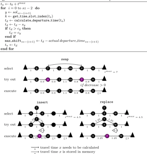
After the construction ofmax antssolutions, the local search moves explained below and displayed in Figure 2 are executed on each constructed solution. For these examples a service time equal to zero is assumed.
4.5 Calculation of the local evaluation metric
As in the ACS for the TD-OP, a local evaluation metric is used to prevent a global and time-consuming evaluation of a solution after every insertion and replacement attempt (Section 4.7 and 4.8). In short, the maximum amount of time that a visit to any given vertex in the current solution can be postponed before the solution becomes infeasible is stored. The calculation of this metric called max shift, is now adapted to take into account the time window restrictions and is presented in the pseudo code of Algorithm 2. Note that in this procedure,sz is the number of vertices stored in solutionsol. Themax shiftmetric is calculated from the last vertex to the first vertex. The arrival time at the end depot is set equal to the latest feasible arrival time. Based on this arrival time the matching departure time is calculated. Afterwards, it is checked if the departure time (after subtracting the service time), which can only be shifted towards the end of the solution sequence, is greater than the closing time of the departing vertex. If this is the case, the departure time is set equal to the closing time. Themax shiftvalue is calculated for every vertex of the solution except the start vertex.
Algorithm 2Calculation ofmax shiftfor TD-OPTW - input:sol ta←t0+tmax
for i= 0 tosz−2 do
y←solsz−(i+1)
k←get time slot index(ta)
td←calculate departure time(ta)
td←td−sy iftd> cythen
td=cy end if
max shiftsz−(i+1)←td−actual departure timesz−(i+1)
ta←td end for swap select try out execute , k, 1 , y 1 , l 1 , m 1 , z 1 , n 1 , 1 tmax= 7 , k, 1 , z 0.9 , l 0.9 , m 1.1 , y 0.8 , n 0.8 , 1 if decrease >0 , k, 1 , z 0.9 , l 0.9 , m 1.1 , y 0.8 , n 0.8 , ≤1 insert select try out execute , y , x, 1 , z 1 , 1 , 1 tmax= 4.5 , x, 1 , z 1 , 1 , 1 , y 0.75 0.75 0.5 , x, 1 , y z, , ≤1 0.75 0.75 , ≤1 replace , y , x, 1 , z 1 , w 1 , 1 tmax= 4.5 , y , x, 1 , z 1 , w 1 , 1 1.25 1.25 0.5 , x, 1 , y 1.25 , w 1.25 , ≤1
travel timexneeds to be calculated x
travel timexis stored in memory x
x max shiftxof the vertex
Fig. 2 Overview of the time-dependent local search moves
4.6 Swap local search move
The swap local search move tries to exchange two vertices in the solution se-quence in order to save travel time. We define y and z as the vertices that will be exchanged,kandl as the predecessor and successor ofy andmandnas the predecessor and successor ofz. After checking thatkandlare neighbours ofzand thatmandnare neighbours ofy, the verticesy andzare temporary exchanged. Otherwise, this swap pair (y, z) is discarded before further evaluation. Afterwards, the new arrival time for the vertices betweenkandnis calculated while account-ing for time window restrictions. Next, the difference in travel time (calculated fromkton) of the possible swap is calculated and if this difference (local gain in travel time) is negative, the swap is executed. However, it is unsure that this exact difference in travel time can be kept until the end of the solution sequence due
to waiting times and the time-dependent nature of succeeding travel times after vertex n(global gain in travel time). However, since our travel time is FIFO we are sure that departing earlier at vertexnguarantees that our new arrival time at the end vertex will be less than or equal to the previous one. Therefore this ap-proach is chosen to avoid a complete evaluation of the solution. This significantly speeds up the search for feasible swap partners. Afterwards, the new arrival times are calculated and themax shiftvalues for the vertices starting fromnuntil the end of the solution can be updated. The update of themax shiftvariable is not recalculated from scratch but is rather based on the following formula:
max shifti =max shifti+ (previous tdi−new tdi) (14) Finally, themax shiftvariable needs to be recalculated for all vertices beforey.
Since this local search move does not use themax shiftlocal evaluation metric, a lot of travel time calculations are needed and therefore the procedure is executed in a first improvement manner. The procedure stops when no more improvements can be found.
4.7 Insert local search move
The problem-specificinsert local search move iteratively attempts to insert non-included neighbouring vertices into an existing solution, thus improving its total reward. The insert move tries to insert vertices into the current solution if the extra travel time, required to visit this new vertex, is less than the value of max shiftof the succeeding vertex. For example, when the algorithm attempts to insert vertex
y betweenxandz, the extra time-dependent travel time equals:
∆tt=ttx,y,tdx+tty,z,tdy−ttx,z,tdx (15) Note that the procedure first checks if vertexyis a neighbour ofxandz, otherwise this insertion combination is discarded. During the calculation, the required service time and waiting time are added to the arrival time when:
tay < oy or taz< oz (16) The insert move is cancelled when the arrival time atyfromxis greater than the closing time ofy:
tay > cy (17)
Recall that this violation is still possible as the set of neighbours is constructed based on time-independent travel times (Section 4.2). Vertexycan only be inserted into the current solution when the extra travel time is less than or equal to the maximum amount of time a visit to vertexzcan be shifted towards the end of the solution sequence or:
∆tt≤max shiftz (18)
When vertex y is actually included in the solution, the algorithm updates the travel time from x to y, as well as the travel times between the vertices after vertexy. This is necessary, because the insertion of vertexyhas most likely caused a change in waiting and/or travel time on the following arcs in the solution. The
max shift value, the previous travel time and the new travel time of the vertex under consideration:
max shifti=max shifti+ (previoustdi−newtdi). (19) Secondly, for the vertices preceding vertexz only a recalculation of max shiftis required.
As a result of this procedure, the computation time needed to check if a vertex can be included or not, and actually executing a feasible insertion is drastically reduced. A visual overview on which travel times are calculated and which are stored in memory is provided in Figure 2.
The insert move is executed in a best-improving manner and stops when no more feasible improvements can be found. The best improving combination is found using a ratio equal to the increase in reward divided by the increase in travel time of a feasible insertion. If the travel time decreases or stays the same, the ratio is set equal to:
(1−∆tt)∗ry. (20)
This means that as ∆tt becomes more and more negative, (1−∆tt) becomes more and more positive, thus artificially increasing the reward.
4.8 Replace local search move
After the insert local search move, the replace move is executed. This move tries to replace a vertex from the current solution with a non-included vertex with a higher reward at the same position in the solution sequence. We definey as the potential replacement vertex to include, z as the vertex in the current solution that will be replaced and x andw respectively as the predecessor and successor ofz. The reward ofz is compared with the reward of its neighbours. When the reward of a non-included neighbour (y) is higher, it is checked if the potential replacement is feasible. A replacement is possible whenyis a neighbour of bothx
andw and when the following inequality is valid:
∆tt≤max shiftw (21)
∆tt= (ttx,y,tdx+tty,w,tdy)−(ttx,z,tdx+ttz,w,tdz) (22) During the calculation of these components, a waiting time is added to the travel time when:
tay < oy or taw< ow (23) The replace move is cancelled when the following inequality is valid:
tay > cy (24)
As soon as a feasible replacement option is found, it is performed (first improve-ment manner). Afterwards, the travel time is recalculated for vertices afterywhile themax shiftvariable is recalculated for vertices beforeyand updated for vertices aftery. The replace move is repeated for each vertex in the solution until no more feasible improvements can be found.
4.9 Update global best
After the construction and local search moves, the algorithm checks which solution has the highest solution reward and stores it as the iteration best solution (solib). If its reward is better than the best reward found during the previous iterations (solgb), we update solgb. If not, variableNni, that keeps track of the number of iterations without improvement, is incremented. When solgb is updated, Nni is reset to 0.
4.10 Global Pheromone update
IfNniis less than a maximum threshold (Nnimax), the pheromone values of the arcs, used insolib, are augmented with the value ofτinit. This makes it more likely that these arcs will be used in a subsequent construction procedure (intensification):
τi−1,i←τi−1,i+τinit ∀i∈solib|i >1 (25) IfNni equalsNnimax, all the pheromone values are reset toτinit. This means that all arcs have again an equal probability to be chosen during the next construction procedure, allowing diversification.
5 Datasets
A set of realistic problem instances was developed based on the road network (G= (V, A)) of the Benelux (Belgium, The Netherlands and Luxembourg) containing 425,479 vertices (V) and 519,915 arcs (A). The historical travel time dataset, consisting of accurately recorded travel time observations every 15 minutes for a representative Tuesday, is used to calculate the travel time for each arc. The travel time dataset is recorded for a road network that covers all highways and frequently travelled roads using the floating car system developed by Be-Mobile (Be-Mobile, 2014). The system uses vehicle probes (e.g., taxi’s, commercial vehicles, private cars, etc.) that communicate their position frequently to a central system. The individual data samples are processed to generate a traffic state for each individual road segment. The system is fully operational since October 2007.
More specifically, there are travel time estimates for 96 time periods k ∈K
per day (with a duration of 15 minutes) for each arc and each arc has a time-independent free-flow tti,j estimate, which is the smallest travel time needed to traverse the arc.
A set of instances was created by randomly selecting respectively 20, 50 and 100 vertices (Vc⊆V) out of this road network and providing them with a reward, opening and closing time and a service time. The other vertices (V \Vc) in the graph can not be visited but might be traversed to reach the vertices inVc. Two vertices out ofVcare selected as start and end depot.
The reward for each regular vertex is generated by selecting a random number from 1 to 30. The deterministic service time of each regular vertex is generated using a random number from a normal distribution with a mean equal to 20 minutes and a standard deviation equal to 5 minutes. The reward of both depots is set equal to 0. The opening time of the start and end depot (o1, ov) is set equal
to 6 am. Furthermore, for each set of vertices, 4 variations intmax(8, 10, 12 and 14 h), resulting in 4 corresponding closing times of the depots (2, 4, 6 and 8pm), and 3 random variations in time window widths (small, medium and large) were created. In total 36 problem instances were created which can be found at the following url:http://www.mech.kuleuven.be/en/cib/op/.
The time-independent and time-dependent travel times of the correspond-ing graph are constructed before the start of the solution procedure. The time-independent travel time (tt) between each pair of verticesVc ⊆V, is calculated using Dijkstra’s shortest path algorithm (using binary heaps) and assuming that arcs can be traversed at their free flow estimates.
The set of time-dependent travel times is calculated by repeatedly using an adapted version of Dijkstra’s algorithm with a departure time equal to the start of a time slot. The number of time slotsκis set equal to the number of time periods
K. To lower the execution time, the travel time profiles are only calculated from each vertexi∈Vcto its set of neighbours (this set is defined in Section 4.2) for all start times equal to the lower limit of all the time slots that are part of the feasible time region. The lower bound of this feasible time region is equal to the start time of the time slot corresponding tooi+si and the upper bound is equal to the end time of the time slot corresponding toci+si.
The resulting time-dependent travel times per time slot are stored for each virtual arc. A virtual arc is a dummy arc that holds a concatenation of arcs con-necting two vertices inVc. The use of virtual arcs to handle complex road networks was originally discussed by Donati et al (2008).
When calculating the travel time for a departure at time td with a shortest path algorithm, the travel time obtained is the right one iftd is equal to the lower limit of a time slot. However, during the execution of the metaheuristic, these travel time distributions are interpolated for moments in time between two such lower limits. As this is an estimation of the travel time, the shortest path when departing at the lower limit of time slottin the virtual arc, might differ from the actual shortest path for departure timestd∈]tst, tst[. In short, the concatenation of arcs that forms the virtual arc might no longer be the shortest path when the departure time is later than the start of the time slot. Apart from the fact that initial experiments showed that this error was very small, no infeasible solutions were encountered during any of our experiments. There is no guarantee in general since the best route can change for every departure time. However when using a large number of time slots, as it is done in this paper, this effect is mitigated.
After these steps, a new virtual network has been constructed. This network corresponds to a complete graph which consists of vertices representing customer locations to visit and virtual arcs with a fixed set of travel time estimates which model the travel time behaviour on a concatenation of real arcs. For simplicity, the term arci, j is used in the remainder of this text for the virtual arc betweeni
andj.
As an indication of the performance of the preprocessing procedure: computa-tional times of 2, 5 and 11 minutes are required on instances with respectively 20, 50 and 100 vertices.
6 Results and Discussion
In this section the performance of the proposed algorithm will be discussed using various tests. In Subsection 6.1 the results of the ACS are compared against known optimal solutions. Since only a few instances could be solved to optimality, a set of artificial benchmarks are devised in Subsection 6.2. In Subsection 6.3 the ACS is compared against a state-of-the-art solution method for the TD-TOPTW. This section is concluded with an overview of the parameter sensitivity in Subsection 6.4 and the (negative) impact of not accounting for time-dependent travel times is shown in Subsection 6.5.
6.1 Comparison to optimal solutions of small instances
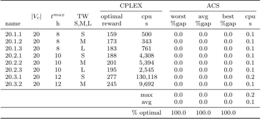
The first experiment consists of a straightforward comparison of the results of the ACS and the optimal solution found by solving the MIP model for TD-OPTW from Section 3. However, most of the time-dependent instances discussed in Sec-tion 5 are too complex to be solved with the MIP using a commercial solver. Since this is not the focus of our research, only a basic implementation of this MIP was implemented using the commercial solver, CPLEX 12.6 (64-bit) using ahigh per-formance computing (HPC) infrastructure which consists of 48 Intel Xeon X5675 3.07 GHz processors and a total of 384 GB of memory. The comparison between the results of these optimal solutions and the ACS for five independent runs is displayed in Table 1. The labels S, M, L stand for the span (closing time minus opening time) of the time windows (small, medium, large).
As performance metrics, the CPU is used together with the percentage gap between the total reward of the optimal solution and the total reward of the heuristic solution:
% gap = optimal reward−heuristic reward
optimal reward ∗100 (26)
The average, the best and the worst gap over all instances is recorded. The ACS is executed until 10,000 trial solutions have been created. The exact number of iterationsNcis therefore adjusted to the value ofmax ants. For example when 20 ants are used, 500 iterations were allowed in order to generate 10,000 trial solutions. The results show the validity of our MIP model but also the excessive time needed to solve these small instances using a commercial solver and a straightforward MIP formulation. Apart from the number of vertices in the problem instance, the required computation time depends first on the value of tmaxand second on the span of the time windows. This table shows that the ACS produces the optimal solution for each run on each instance in very short computations times.
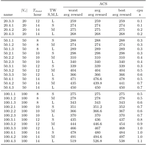
The reward of the ACS for the instances without known optimal solution are also displayed in Table 10 to allow for future benchmarking.
6.2 Comparison to known optimal solutions of large instances
To evaluate the performance of our TD-OPTW metaheuristic, it would be useful to have an optimal solution for each benchmark instance. However, the time-dependent instances are too complex to be solved with a commercial solver and a
Table 1 Comparison with optimal solutions of small instances
CPLEX ACS
|Vc| tmax TW optimal cpu worst avg best cpu
name h S,M,L reward s %gap %gap %gap s
20.1.1 20 8 S 159 500 0.0 0.0 0.0 0.1 20.1.2 20 8 M 173 343 0.0 0.0 0.0 0.1 20.1.3 20 8 L 183 761 0.0 0.0 0.0 0.1 20.2.1 20 10 S 188 4,308 0.0 0.0 0.0 0.1 20.2.2 20 10 M 201 5,394 0.0 0.0 0.0 0.1 20.2.3 20 10 L 195 2,545 0.0 0.0 0.0 0.1 20.3.1 20 12 S 277 130,118 0.0 0.0 0.0 0.2 20.3.2 20 12 M 245 9,692 0.0 0.0 0.0 0.1 max 0.0 0.0 0.0 0.2 avg 0.0 0.0 0.0 0.1 % optimal 100.0 100.0 100.0
straightforward MIP formulation. Therefore, a procedure is developed which allows to test the proposed algorithm on larger instances with known optimal solutions. Firstly, all instances were solved as time-independent OPTWs using the HPC infrastructure with 48 Intel Xeon X5675 3.07 GHz processors and a total of 384 GB of memory. The MIP formulation of the OPTW in Vansteenwegen et al (2011a) was used to find these optimal solutions. The obtained solutions together with their corresponding computation times is available at:http://www.mech.kuleuven.be/ en/cib/op/.
The excessive resources and CPU time needed to solve these time-independent OP instances, illustrates that it would be pointless to solve the datasets as time-dependent OPTWs. The found (near-)optimal solutions are displayed in Table 2 (column “optimal”). If the optimal solution could not be found, the best solution after 72 hours of computation time is taken as the benchmark. These instances are marked with a star in the column “name”. Following the optimization by CPLEX, the optimal time-independent solutions (sequence of vertices) are used to modify the original dependent instances in such a way that slightly modified time-dependent instances with known (near-)optimal solutions are created using the procedure described in (Verbeeck et al, 2014).
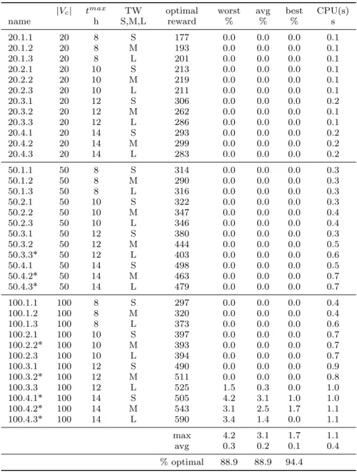
The creation of the benchmark instances in this way allows to compare the performance of the developed solution methods with known optimal solutions for larger instances. For five independent runs of the algorithm, these results are displayed in Table 2. In Table 3 the % gap per dataset is displayed.
These results prove the high performance quality of the ACS, since the average gap is very low, i.e. only 0.2%. Furthermore, the known optimal solution was found for 32 out of 36 test instances. A second conclusion is that the average gap increases as the test instances become more complex due to a longer travel time limit and an increasing number of vertices. Studying the computation time leads to the conclusion that the ACS is very fast, as on average only 0.4 seconds are needed to obtain a solution. The maximum observed CPU time was 1.1 second, which is more than fast enough for most application purposes. Therefore, it can be
Table 2 Results for the TD-OPTW per problem instance
|Vc| tmax TW optimal worst avg best CPU(s)
name h S,M,L reward % % % s 20.1.1 20 8 S 177 0.0 0.0 0.0 0.1 20.1.2 20 8 M 193 0.0 0.0 0.0 0.1 20.1.3 20 8 L 201 0.0 0.0 0.0 0.1 20.2.1 20 10 S 213 0.0 0.0 0.0 0.1 20.2.2 20 10 M 219 0.0 0.0 0.0 0.1 20.2.3 20 10 L 211 0.0 0.0 0.0 0.1 20.3.1 20 12 S 306 0.0 0.0 0.0 0.2 20.3.2 20 12 M 262 0.0 0.0 0.0 0.1 20.3.3 20 12 L 286 0.0 0.0 0.0 0.1 20.4.1 20 14 S 293 0.0 0.0 0.0 0.2 20.4.2 20 14 M 299 0.0 0.0 0.0 0.2 20.4.3 20 14 L 283 0.0 0.0 0.0 0.2 50.1.1 50 8 S 314 0.0 0.0 0.0 0.3 50.1.2 50 8 M 290 0.0 0.0 0.0 0.3 50.1.3 50 8 L 316 0.0 0.0 0.0 0.3 50.2.1 50 10 S 322 0.0 0.0 0.0 0.3 50.2.2 50 10 M 347 0.0 0.0 0.0 0.4 50.2.3 50 10 L 346 0.0 0.0 0.0 0.4 50.3.1 50 12 S 380 0.0 0.0 0.0 0.3 50.3.2 50 12 M 444 0.0 0.0 0.0 0.5 50.3.3* 50 12 L 403 0.0 0.0 0.0 0.6 50.4.1 50 14 S 498 0.0 0.0 0.0 0.5 50.4.2* 50 14 M 463 0.0 0.0 0.0 0.7 50.4.3* 50 14 L 479 0.0 0.0 0.0 0.7 100.1.1 100 8 S 297 0.0 0.0 0.0 0.4 100.1.2 100 8 M 320 0.0 0.0 0.0 0.4 100.1.3 100 8 L 373 0.0 0.0 0.0 0.6 100.2.1 100 10 S 397 0.0 0.0 0.0 0.7 100.2.2* 100 10 M 393 0.0 0.0 0.0 0.7 100.2.3 100 10 L 394 0.0 0.0 0.0 0.7 100.3.1 100 12 S 490 0.0 0.0 0.0 0.9 100.3.2* 100 12 M 511 0.0 0.0 0.0 0.8 100.3.3 100 12 L 525 1.5 0.3 0.0 1.0 100.4.1* 100 14 S 505 4.2 3.1 1.0 1.0 100.4.2* 100 14 M 543 3.1 2.5 1.7 1.1 100.4.3* 100 14 L 590 3.4 1.4 0.0 1.1 max 4.2 3.1 1.7 1.1 avg 0.3 0.2 0.1 0.4 % optimal 88.9 88.9 94.4
Table 3 % gap (best, average, worst) and average CPU time per dataset best avg worst CPU |Vc| % gap % gap % gap s
20 0.0 0.0 0.0 0.1
50 0.0 0.0 0.0 0.4
concluded that the ACS is able to deliver a high performance requiring a minimal computational effort.
6.3 Comparison to a state-of-the-art solution procedure
The iterated local search method (ILS) of Garcia et al (2013) was developed for the TD-TOPTW and is, apart from the complex algorithm of Abbaspour and Samadzadegan (2011), the only practical algorithm that is capable to deal with time-dependency. Since this ILS method exploits the fixed frequency of buses to perform quick arrival and departure time updates, it is not capable to deal with time-dependency originating from congestion on the arcs. Therefore, the ILS was reimplemented with a few modifications. Firstly, the local evaluation metric and solution update procedure described in Section 4.7 was used. Secondly, after the shake procedure, the solution is completely evaluated since it turned out to be too time expensive to verify which parts of the solution sequence needed to be updated and to execute the partial updates afterwards. These issues, together with other implementation details like not making use of parallel computing due to the sequential structure of ILS, results in greater computational times for the ILS method compared to the ACS. It should be noted that these issues contributed to the choice of the ACS as the preferred solution framework in the first place.
The performance of the ILS and ACS, both with 10,000 trial solutions is sim-ilar when used to solve all the instances as time-independentOPTWs. The ILS achieved an average gap of 0.22%, a maximum gap of 4% and an average cpu time of 1.95 seconds. The performance of the ACO consists of an average gap of 0.10%, a maximum gap of 3% and an average cpu time of 0.46 seconds. These results also show the good performance of both heuristics when used as a solution method for the regular OPTW.
The results of ILS and ACS when applied to time-dependent instances, both with 10,000 trial solutions, are compared and can be found in Table 4. More de-tailed results can be found at http://www.mech.kuleuven.be/en/cib/op/. The first two columns display the average computational time of both solution proce-dures and the third column displays the gap defined as:
gap= ILSreward−ACSreward
ILSreward (27)
On average the performance of the ACS is 6.2% better than that of the ILS. Furthermore, the detailed results show that the ILS could not improve the reward of the ACS solution method on a single instance. Finally, we also compared the performance of the ILS after 50,000 solutions with the results of the ACS after 10,000 trial solutions and noticed the same performance gap of 6.2% which might indicate that the ILS more easily gets stuck in local optima. Secondly, iteratively removing vertices from a solution turns out to be impractical and time consuming.
6.4 Sensitivity Analysis
Table 5 provides an overview of the input parameters of ACS, including their value used during all the discussed experiments. These values were determined
Table 4 Comparison of ACS to a state-of-the-art technique after 10,000 solutions ACS cpu ILS cpu gap
|Vc| s s %
20 0.1 0.1 -3.8%
50 0.4 0.6 -8.7%
100 0.8 2.4 -6.0%
Overall 0.4 1.1 -6.2%
Table 5 Overview of the input parameters TD-OPTW
Input parameter Description Value
τinit initial pheromone value 1
α importance of pheromone information 4
β importance of heuristic information 1
max ants number of solutions that is constructed and improved per iteration 50
ρ evaporation rate 0.05
Nmax
ni maximum number of iterations without improvement (% ofNc) 25%
Table 6 Effect ofα,β,Nmax
ni ,ρ, andmax antson the average gap
α % gap 1 2.9 3 1.1 6 1.1 9 1.5 Total 1.7 β % gap 1 0.7 3 0.8 6 1.6 9 3.4 Total 1.7 Nmax ni % gap 0.25 1.5 0.50 1.6 0.75 1.7 1.00 1.8 Total 1.7 ρ % gap 0.01 2.6 0.05 1.2 0.10 1.2 Total 1.7
max ants % gap
10 2.8 25 1.8 50 1.2 75 1.2 100 1.2 Total 1.7
Table 7 Effect on the % gap and average CPU time (s) of different design components
Metric S I R - - - S - - - I - - - R - I R S I - S - R
max % gap 3.1 30.6 24.5 12.7 26.7 9.5 7.6 24.3
avg % gap 0.2 10.6 8.8 2.4 9.7 0.8 0.8 0.8
avg cpu 0.4 0.1 0.2 0.4 0.2 0.4 0.4 0.2
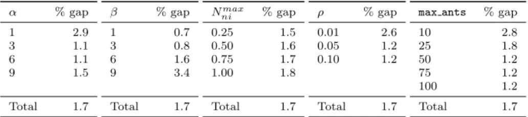
after preliminary tests. A sensitivity study is performed to measure the impact on the performance for various combinations of input parameter values. The results are displayed in Table 6. The significant input parameters that have an impact on the performance, based on an ANOVA test, areα,β,ρandmax ants.
Table 7 provides insights into the performance of some design decisions. These effects are measured by leaving out some or all of the 3 local search moves (S: swap, I: insert, R: replace) and repeating the test procedure discussed in Section 6.2. The missing components in the ACS framework (Algorithm 1) are marked with a ”-”. Mainly based on the average gap, we conclude that the strength of the ACS lies in the interaction effect between the swap, insert and replace local search moves.
6.5 Impact of time-dependent travel times
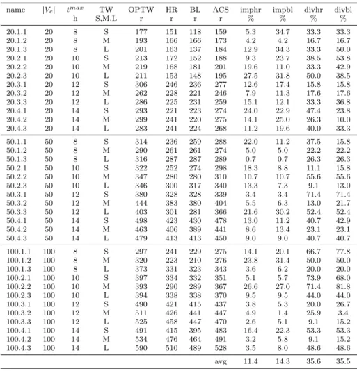
In order to measure the impact of ignoring the time-dependency of travel times when dealing with practical problems, the optimal OPTW solutions are evaluated in a time-dependent context. This means that all travel times, arrival times and departure times are updated. Two events can turn a solution infeasible: a violation of the time window at a regular vertex and secondly, arriving too late at the end vertex.
Two different repair algorithms are proposed that inspect the solution sequence (starting from the start vertex to the end vertex) and implement different recourse actions. The first algorithm is calledheuristic repair and removes the first vertex with a violated time window and inspects the solution again for further violations. When a late arrival occurs at the end vertex, the vertex with the lowest reward in the solution sequence is removed and the solution is again inspected for further violations. Vertices are eligible for removal only if no waiting occurs at subsequent vertices in the solution sequence. The reason for this is that removing a vertex which is positioned before a vertex where waiting occurs, would not lead to a decrease of the total travel time as it would only lead to an increase in waiting time at the subsequent vertex. The second algorithm is calledbusiness logic repair and also removes the first vertex with a violated time window and afterwards inspects the solution again for further violations. For a late arrival at the end vertex, however, the last regular vertex of the solution sequence is removed and the solution is inspected for further violations. This last recourse action is chosen because it might resemble the action of actual planners in logistics companies. The last customers on a trip are more likely to be removed when it becomes clear that the driver is falling behind schedule and wants to return to the end depot. Finally, OPTW solutions, evaluated by both algorithms, are compared against the TD-OPTW solutions generated by the ACS.
The results are displayed in Tables 8 and 9. The first four columns list re-spectively the name, number of vertices, maximum allowed total travel time, time window span of the problem instance and the total reward of the optimal OPTW instance. The next two columns display respectively the reward of the evaluated optimal OPTW solution by the heuristic repair (HR) and the business logic re-pair (BL). In the 8th column the reward of the time-dependent OPTW solution produced by the ACS is given. Finally, the last four columns display the % im-provement (imphr and impbl) and the diversity in the solution sequences (divhr and divbl) of the ACS as compared with HR and BL strategies. The diversity between two solutions A and B is calculated as the sum of the number of ver-tices in A not present in B and the number of verver-tices in B not present in A, divided by the total number of vertices present in A and B (start and end vertex not included). The results are road network specific but nonetheless stress the se-vere impact of congestion on the quality and structure of the proposed solutions. Apparently there seems to be no strong connection between the degree of improve-ment and diversity, on the one hand, and the most important instance parameters like the number of vertices, tmax and the time window span on the other hand. However, instances with smaller time windows are more likely to become infeasible and therefore the improvement of using the ACS is more important. A possible explanation for the greater impact of congestion for the instances with 100 vertices
is that the routes for these problems are more complex and are therefore also more vulnerable to congestion.
An overall conclusion concerning the diversity of the routes proposed for both problems is that a ”good” route for the TD-OPTW differs significantly from the optimal route for the OPTW. This strengthens the claim that time-independent route planning is not appropriate in a time-dependent business context. These results also show that using a time-independent routing planner together with some basic recourse actions, that are often used in practice in order to deal with time-dependent disturbance, does not work out well. Time-independent routes cannot be easily altered or transformed into robust routes that have some ”buffer” against the negative effects of time-dependent disturbance since congestion is a time-spatial phenomenon.
Table 8 Impact of time-dependency per problem instance
name |Vc| tmax TW OPTW HR BL ACS imphr impbl divhr divbl
h S,M,L r r r r % % % % 20.1.1 20 8 S 177 151 118 159 5.3 34.7 33.3 33.3 20.1.2 20 8 M 193 166 166 173 4.2 4.2 16.7 16.7 20.1.3 20 8 L 201 163 137 184 12.9 34.3 33.3 50.0 20.2.1 20 10 S 213 172 152 188 9.3 23.7 38.5 53.8 20.2.2 20 10 M 219 168 181 201 19.6 11.0 33.3 42.9 20.2.3 20 10 L 211 153 148 195 27.5 31.8 50.0 38.5 20.3.1 20 12 S 306 246 236 277 12.6 17.4 15.8 15.8 20.3.2 20 12 M 262 228 221 246 7.9 11.3 17.6 17.6 20.3.3 20 12 L 286 225 231 259 15.1 12.1 33.3 36.8 20.4.1 20 14 S 293 221 223 274 24.0 22.9 47.4 23.8 20.4.2 20 14 M 299 241 220 275 14.1 25.0 26.3 10.0 20.4.3 20 14 L 283 241 224 268 11.2 19.6 40.0 33.3 50.1.1 50 8 S 314 236 259 288 22.0 11.2 37.5 15.8 50.1.2 50 8 M 290 261 261 274 5.0 5.0 22.2 22.2 50.1.3 50 8 L 316 287 287 289 0.7 0.7 26.3 26.3 50.2.1 50 10 S 322 252 274 298 18.3 8.8 11.1 15.8 50.2.2 50 10 M 347 280 280 310 10.7 10.7 55.6 55.6 50.2.3 50 10 L 346 300 317 340 13.3 7.3 9.1 13.0 50.3.1 50 12 S 380 328 328 339 3.4 3.4 71.4 71.4 50.3.2 50 12 M 444 383 380 404 5.5 6.3 13.0 21.7 50.3.3 50 12 L 403 301 281 366 21.6 30.2 52.4 52.4 50.4.1 50 14 S 498 423 430 478 13.0 11.2 40.7 42.9 50.4.2 50 14 M 463 406 389 441 8.6 13.4 23.1 23.1 50.4.3 50 14 L 479 413 413 450 9.0 9.0 40.7 40.7 100.1.1 100 8 S 297 241 229 275 14.1 20.1 66.7 77.8 100.1.2 100 8 M 320 223 210 276 23.8 31.4 50.0 50.0 100.1.3 100 8 L 373 331 323 343 3.6 6.2 20.0 20.0 100.2.1 100 10 S 397 334 332 351 5.1 5.7 73.9 68.0 100.2.2 100 10 M 393 290 289 367 26.6 27.0 71.4 81.8 100.2.3 100 10 L 394 338 338 370 9.5 9.5 44.0 44.0 100.3.1 100 12 S 490 421 415 437 3.8 5.3 20.0 26.7 100.3.2 100 12 M 511 426 441 447 4.9 1.4 25.9 3.4 100.3.3 100 12 L 525 458 447 470 2.6 5.1 9.1 15.2 100.4.1 100 14 S 491 415 395 483 16.4 22.3 53.3 53.3 100.4.2 100 14 M 534 476 464 491 3.2 5.8 9.1 15.2 100.4.3 100 14 L 590 510 489 528 3.5 8.0 48.6 48.6 avg 11.4 14.3 35.6 35.5
Table 9 Impact of time-dependency (heuristic repair) versus problem characteristics
|Vc| %imphr %divhr tmax %imphr %divhr TW %imphr %divhr
20 14.5 32.1 8 12.7 34.0 S 16.3 42.5
50 12.8 33.6 10 17.2 43.0 M 11.7 30.4
100 11.5 41.0 12 9.3 28.7 L 10.9 33.9
14 12.6 36.6
7 Conclusion
This paper has discussed the orienteering problem, in particular the extension where time windows are considered together with time-dependent travel times leading to the time-dependent orienteering problem with time windows (TD-OPTW). In the considered tourist and logistical applications, this modification models multi-modal transport functionality, as well as vehicle routing planning that takes congestion into account. Most of these applications require solutions within a short amount of computation time.
In this paper, a mixed integer problem formulation and a metaheuristic based on an ant colony system are proposed. The metaheuristic uses the following time-dependent local search moves: insert, replace and swap. The evaluation of possible improvement moves is speeded up by a local evaluation metric and by efficiently limiting the number of vertices that are considered.
Moreover, realistic time-dependent test instances with known optimal solutions are developed and made publicly available. A total of 36 test instances with a number of vertices to visit ranging from 20 to 100 were extracted from a road network containing 84,720 vertices and 116,683 arcs.
The TD-OPTW algorithm obtains very good results on these benchmark in-stances, requiring small computation times due to the combination of a well per-forming metaheuristic framework and the interaction effect between three efficient local search procedures tailored to the problem characteristics. The average reward gap with the known optimal solution on these test instances is only 0.2% with an average computation time of 0.4 seconds. A comparison between the ACS and a state-of-the-art technique showed that the performance of the latter is 6.2% worse. The impact of not accounting for time-dependency on the proposed network is on average 12.9%. Finally, there is a significant difference (35.6%) between the struc-ture of the solution sequence of a time-dependent solution and a solution ignoring time-dependency. These results also showed that some basic recourse actions which are often used in practice to create a kind of ”buffer” for the time-dependent dis-turbance do not pay off.
Further research could focus on the time-dependent variant of the team orien-teering problem (TD-TOPTW). This rather interesting extension of the problem allows to optimize the routing of a fleet of vehicles, instead of only one vehi-cle. Secondly, in this paper, we have ignored the fact that customers (vertices) not served today must be served in the near future. Including this consideration would make for an interesting extension and could have a big impact on which customers are selected on a given day. Thirdly, in general, congestion causes two undesirable effects to the transportation users: on one hand it causes an increase of expected travel time due to a reduction of the mean speed and queuing, and on
the other hand it increases the variability of travel times. Therefore, in a realistic road network, travel times are both time-dependent and stochastic. Therefore, an interesting challenge would be to solve an orienteering problem variant in which the travel time between two locations is a stochastic function that depends on the departure time at the first location.
Acknowledgments
This research was funded by the Agency for Innovation by Science and Technology in Flanders (IWT).
The computational resources (Stevin Supercomputer Infrastructure) and ser-vices used in this work were provided by the VSC (Flemish Supercomputer Cen-ter), funded by Ghent University, the Hercules Foundation and the Flemish Gov-ernment – department EWI.
References
Abbaspour A, Samadzadegan F (2011) Time-dependent personal tour planning and scheduling in metropolises. Expert Systems with Applications 38:12,439– 12,452
Aghezzaf EH, Zhong Y, Raa B, Mateo M (2012) Analysis of the single-vehicle cyclic inventory routing problem. International Journal of Systems Science 43(11):2040–2049
Balseiro S, Loisea I, Ramonet J (2011) An ant colony algorithm hybridized with insertion heuristic for the time dependent vehicle routing problem with time windows. Computers & Operations Research 38(6):954–966
Be-Mobile (2014) Be-mobile: Floating vehicle data.http://www.be-mobile.be
Chao I, Golden B, Wasil E (1996) Theory and methodology a fast and effective heuristic for the orienteering problem. European Journal of Operational Re-search 88:475–489
Chen H, Hsueh C, Chang M (2006) The real-time time-dependent vehicle routing problem. Transportation Research Part E 42:383–408
Donati A, Montemanni R, Casagrande N, Rizzoli A, Gambardella L (2008) Time dependent vehicle routing problem with a multi ant colony system. European Journal of Operational Research 185:1174–1191
Evers L, Glorie K, van der Ster S, Barros A, Monsuur H (2012) The orienteer-ing problem under uncertainty stochastic programmorienteer-ing and robust optimization compared. Tech. Rep. Econometric Institute Report EI 2012-21, Erasmus Uni-versity, Econometric Institute, URLhttp://hdl.handle.net/1765/37193
Fomin F, Lingas A (2002) Approximation algorithms for time-dependent orien-teering. Information Processing Letters 83:57–62
Garcia A, Vansteenwegen P, Arbelaitz O, Souffriau W, Linaza M (2013) Integrat-ing Public Transportation in Personalised Electronic Tourist Guides. Computers & Operations Research 40:758–774
Gavalas D, Konstantopoulos C, Mastakas K, Pantziou G, Vathis N (2014) Efficient heuristics for the time dependent team orienteering problem with time windows.
In: Gupta P, Zaroliagis C (eds) Applied Algorithms, Lecture Notes in Computer Science, vol 8321, Springer International Publishing, pp 152–163
Gavalas D, Konstantopoulos C, Mastakas K, Pantziou G, Vathis N (2015) Heuris-tics for the time dependent team orienteering problem: Application to tourist route planning. Computers & Operations Research 62(0):36 – 50
Golden B, Levy L, Vohra R (1987) The orienteering problem. Naval Research Logistics 34:307–318
Gunawan A, Lau H, Vansteenwegen P (2016) Orienteering problem: a survey of recent variants, solution approaches and applications. European Journal of Op-erational Research: accepted
Haghani A, Jung S (2005) A dynamic vehicle routing problem with time-dependent travel times. Computers & Operations Research 32:2959–2986
Hashimoto H, Yagiurab M, Ibaraki T (2008) An iterated local search algorithm for the time-dependent vehicle routing problem with time windows. Discrete Optimization 5:434–456
Ichoua S, Gendreau M, Potvin JY (2003) Vehicle dispatching with time-dependent travel times. European Journal of Operational Research 144:379–396
Kantor M, Rosenwein M (1992) The orienteering problem with time windows. Journal of Operational Research Society 43 (6):629–635
Ke L, Archetti C, Feng Z (2008) Ants can solve the team orienteering problem. Computers and Industrial Engineering 54:648–665
Kok AL, Hans EW, Schutten JMJ (2012) Vehicle routing under time-dependent travel times: The impact of congestion avoidance. Computers & Operations Research 39 (5):910–918
Kritzinger S, Tricoire F, Doerner K, Hartl R (2011) Variable neighborhood search for the time-dependent vehicle routing problem with soft time windows. In: Coello C (ed) Learning and Intelligent Optimization, Lecture Notes in Computer Science, vol 6683, Springer Berlin Heidelberg, pp 61–75
Lecluyse C, Van Woensel T, Peremans H (2009) Vehicle routing with stochastic time-dependent travel times. 4OR: Quarterly journal of Operational Research 7:363–377
Li J (2011) Model and algorithm for time-dependent team orienteering problem. In: Lin S, Huang X (eds) Advanced Research on Computer Education, Simulation and Modeling, Communications in Computer and Information Science, vol 175, Springer Berlin Heidelberg, pp 1–7
Li J, Wu Q, Li X, Zhu D (2010) Study on the time-dependent orienteering prob-lem. In: International Conference on E-Product E-Service and E-Entertainment (ICEEE), pp 1 – 4
Mufalli F, Batta R, Nagi R (2012) Simultaneous sensor selection and routing of unmanned aerial vehicles for complex mission plans. Computers & Operations Research 39(11):2787 – 2799
Potvin J, Xu Y, Benyahia I (2006) Vehicle routing and scheduling with dynamic travel times. Computers & Operations research 33:1129–1137
Royset JO, Reber DN (2009) Optimized routing of unmanned aerial systems for the interdiction of improvised explosive devices. Military Operations Research 14(4):5–19
Schilde M, Doerner K, Hartl R, Kiechle G (2009) Metaheuristics for the biobjective orienteering problem. Swarm Intelligence 3:179–201
Soler D, Albiach J, Martinez E (2009) A way to optimally solve a time-dependent vehicle routing problem with time windows. Operations Research Letters 37:37– 42
S¨orensen K, Sevaux M, Schittekat P (2008) Adaptive and Multilevel Metaheuris-tics, Lecture Notes in Economics and Mathematical Systems, vol 136, Springer, London, chap Multiple neighbourhood search in commercial VRP packages: evolving towards self-adaptive methods, pp 239–253
Souffriau W, Vansteenwegen P, Vertommen J, Vanden Berghe G, Van Oudheusden D (2008) A personalised tourist trip design algorithm for mobile tourist guides. Applied Artificial Intelligence 22:964–985
Tsiligirides T (1984) Heuristic methods applied to orienteering. Journal of the Operational Research Society 35 (9):797–809
Van Woensel T, Kerbache L, Peremans H, Vandaele N (2008) Vehicle routing with dynamic travel times: A queueing approach. European Journal of Operational Research 186:990–1007
Vansteenwegen P, Van Oudheusden D (2007) The mobile tourist guide: An OR opportunity. OR Insights 20 (3):21–27
Vansteenwegen P, Souffriau W, Van Oudheusden D (2011a) The orienteering prob-lem: a survey. European Journal of Operational Research 209:1–10
Vansteenwegen P, Souffriau W, Vanden Berghe G, Van Oudheusden D (2011b) The City Trip Planner: A Tourist Expert System. Expert Systems with Applications 38:6540–6546
Verbeeck C, S¨orensen K, Aghezzaf EH, Vansteenwegen P (2014) A fast solution method for the time-dependent orienteering problem. European Journal of Op-erational Research 236 (2):419–432
Wang X, Golden BL, Wasil EA (2008) The Vehicle Routing Problem: Latest Ad-vances and New Challenges, Springer US, Boston, MA, chap Using a Genetic Algorithm to Solve the Generalized Orienteering Problem, pp 263–274
A Detailed results TD-OPTW
Table 10 Detailed results TD-OPTW
ACS
|Vc| Tmax TW worst avg best cpu
name hour S,M,L avg reward avg reward avg reward s
20.3.3 20 12 L 259 259 259 0.1 20.4.1 20 14 S 274 274 274 0.1 20.4.2 20 14 M 275 275 275 0.2 20.4.3 20 14 L 268 268 268 0.2 50.1.1 50 8 S 288 288 288 0.3 50.1.2 50 8 M 274 274 274 0.3 50.1.3 50 8 L 289 289 289 0.3 50.2.1 50 10 S 298 298 298 0.3 50.2.2 50 10 M 310 310 310 0.4 50.2.3 50 10 L 340 340 340 0.4 50.3.1 50 12 S 339 339 339 0.3 50.3.2 50 12 M 404 404 404 0.5 50.3.3 50 12 L 366 366 366 0.6 50.4.1 50 14 S 471 476.6 478 0.5 50.4.2 50 14 M 435 439.8 441 0.7 50.4.3 50 14 L 450 450 450 0.7 100.1.1 100 8 S 275 275 275 0.5 100.1.2 100 8 M 278 278 278 0.5 100.1.3 100 8 L 343 343 343 0.6 100.2.1 100 10 S 351 351.2 352 0.7 100.2.2 100 10 M 366 366.6 367 0.6 100.2.3 100 10 L 370 370 370 0.7 100.3.1 100 12 S 435 436 437 0.8 100.3.2 100 12 M 444 446.6 454 0.9 100.3.3 100 12 L 466 467 468 1.0 100.4.1 100 14 S 478 480 484 1.0 100.4.2 100 14 M 491 494.6 497 1.0 100.4.3 100 14 L 519 526.8 538 1.1