A New Mask for Automatic Building Detection from High Density Point Cloud Data and Multispectral Imagery

(1)

A NEW MASK FOR AUTOMATIC BUILDING DETECTION FROM HIGH DENSITY

POINT CLOUD DATA AND MULTISPECTRAL IMAGERY

Mohammad Awrangjeb∗, Fasahat U. Siddiqui

Institute for Integrated and Intelligent Systems, Griffith University, Nathan, QLD 4111, Australia Phone: +61 7 373 55032, E-mail: [email protected], [email protected]

Web:www.ict.griffith.edu.au/awrangjeb

KEY WORDS:Building extraction, building mask, building detection, point cloud data, LIDAR, multispectral imagery

ABSTRACT:

In complex urban and residential areas, there are buildings which are not only connected with and/or close to one another but also partially occluded by their surrounding vegetation. Moreover, there may be buildings whose roofs are made of transparent materials. In transparent buildings, there are point returns from both the ground (or materials inside the buildings) and the rooftop. These issues confuse the previously proposed building masks which are generated from either ground points or non-ground points. The normalised digital surface model (nDSM) is generated from the non-ground points and usually it is hard to find individual buildings and trees using the nDSM. In contrast, the primary building mask is produced using the ground points, thereby it misses the transparent rooftops. This paper proposes a new building mask based on the non-ground points. The dominant directions of non-ground lines extracted from the multispectral imagery are estimated. A dummy grid with the target mask resolution is rotated at each dominant direction to obtain the corresponding height values from the non-ground points. Three sub-masks are then generated from the height grid by estimating the gradient function. Two of these sub-masks capture planar surfaces whose height remain constant in along and across the dominant direction, respectively. The third sub-mask contains only the flat surfaces where the height (ideally) remains constant in all directions. All the sub-masks generated in all estimated dominant directions are combined to produce the candidate building mask. Although the application of the gradient function helps in removal of most of the vegetation, the final building mask is obtained through removal of planar vegetation, if any, and tiny isolated false candidates. Experimental results on three Australian data sets show that the proposed method can successfully remove vegetation, thereby separate buildings from occluding vegetation and detect buildings with transparent roof materials. While compared to existing building detection techniques, the proposed technique offers higher object-based completeness, correctness and quality, specially in complex scenes with aforementioned issues. It is not only capable of detecting transparent buildings, but also small garden sheds which are sometimes as small as 5 m2in area.

1. INTRODUCTION

Automatic building detection from remote sensing data has var-ious applications including urban planning and disaster (e.g., bushfire) management. In the literature, a number of building detection techniques have been reported over the last couple of decades. These can be divided into three major groups (Lee et al., 2008). Firstly, there are many algorithms which use 2D or 3D information from photogrammetric imagery. Secondly, there have been several attempts to detect building regions from DAR (LIght Detection And Ranging) data. Finally, since LI-DAR and imagery each have particular advantages and disadvan-tages in horizontal and vertical positioning resolution and accu-racy, several authors have promoted an integration of LIDAR data and imagery as a means of advancing building detection. More specifically, intensity and height information from LIDAR can be used with texture and region boundary information from imagery to improve detection accuracy (Habib et al., 2010). However, the success of automatic building detection is still largely impeded by scene complexity, incomplete cue extraction and sensor de-pendency of data (Sohn and Dowman, 2007). Vegetation, and especially trees, can be the prime cause of scene complexity and incomplete cue extraction. Important building cues can be com-pletely or partially missed due to occlusions and shadowing from trees (Awrangjeb et al., 2012).

Majority of the existing building detection techniques, which in-∗_{Corresponding author}

volve LIDAR data, are based on the two previously proposed building masks: the normalised digital surface model (nDSM) (Rottensteiner et al., 2005) and primary mask (Awrangjeb et al., 2010). The nDSM is generated from the non-ground points and usually it connects neighbouring buildings and trees. Conse-quently, it is hard to find individual buildings and trees using the nDSM. In contrast, the primary building mask is produced using the ground points. Since the ground points represent the ground in this mask, due to ground points returned from the transparent building floors, such buildings are not captured in this mask. This paper proposes a new building mask for automatic building detection from LIDAR data and multispectral imagery. First, ob-jects below a given threshold above the ground, such as bushes, cars and carports, are removed from the raw LIDAR data. Sec-ond, the dominant directions of non-ground lines extracted from the multispectral imagery are estimated. Third, a dummy grid with the target mask resolution is rotated at each dominant di-rection to obtain the height values from the non-ground points. Fourth, three sub-masks are then generated from the height grid by estimating the gradient function. Fifth, all the sub-masks gen-erated in all estimated dominant directions are combined to pro-duce the candidate building mask. Finally, the final building mask is obtained through removal of planar vegetation, if any, and tiny isolated false candidates. In experimentation, a higher object-based performance has been observed when tested on three Aus-tralian data sets, specially in complex scenes with dense vegeta-tion causing shadow and occlusions.

ISPRS Annals of the Photogrammetry, Remote Sensing and Spatial Information Sciences, Volume IV-4/W4, 2017 4th International GeoAdvances Workshop, 14–15 October 2017, Safranbolu, Karabuk, Turkey

(2)

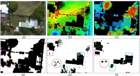
Figure 1. A complex scene: (a) aerial image, (b) ground points, (c) non-ground points, (d) normalised-DSM generated from the non-ground points, (e) primary mask generated from ground points and (f) proposed building mask generated from non-ground points.

2. SEARCH FOR A NEW BUILDING MASK

Figure 1 shows a complex scene, where buildings are not only connected with and partially occluded by their surrounding veg-etation but also they are close to each other. Moreover, there is a building whose roof is made of transparent materials (shown within the pink coloured rectangle). Consequently, for this build-ing there exist both ground and non-ground points (see points within the pink coloured rectangle in Figures 1(b)-(c)). These two phenomena confuse any building masks which are generated from the ground or the non-ground point sets.

Before generating any masks, the nDSM (Rottensteiner et al., 2005) and primary mask (Awrangjeb et al., 2010) apply a height thresholdTh(e.g., the ground height plus 1 m) to the input point-cloud data in order to divide the input data into ground and non-ground point sets. The nDSM, shown in Figure 1(d), is generated using the ground point set in Figure 1(c) and represents non-zero heights indicating the elevated objects aboveTh. As can be seen, buildings and trees are found connected with one another in the nDSM. Thus, it is hard to find the individual buildings using the nDSM. In contrast, the primary mask, shown in Fig-ure 1(e), is generated using the ground point set in FigFig-ure 1(b). In this mask, buildings and trees are found thinner than those in the nDSM. Consequently, individual buildings and vegetation are easily recognisable in the primary mask. However, it has two main problems. Firstly, some vegetation are still found connected with the neighbouring trees (see light blue coloured rectangles in Figure 1(e)). Secondly, the transparent buildings within the pink coloured rectangle is almost missed.

In order to eliminate the aforementioned problems, a new build-ing mask based on the non-ground points is proposed in this pa-per. As shown in Figure 1(f), the new building mask has the fol-lowing advantages. Firstly, any vegetation in the scene is mostly removed. Thus, buildings become easily identifiable. Secondly, buildings with transparent roof materials are detected. Finally, it also detects small garden sheds which are sometimes as small as 5 m2in area.

3. PROPOSED BUILDING DETECTION TECHNIQUE

Figure 2 shows the flow diagram for the proposed new building detection technique. In the following subsections, each step is described in detail.

Figure 2. Flow diagram for new building detection technique.

3.1 Find Non-ground Points

If a Digital Terrain Model (DTM) is not available, one can be generated from the input LIDAR point cloud data using a com-mercial software. We assume that the DTM is given as an input to the proposed technique. Then, for each LIDAR point, the cor-responding DTM height is used as the ground height, Hg. A height thresholdTh=Hg+hc, wherehc is a height constant that separates low height objects from high height objects, is then applied to the LIDAR data (Awrangjeb et al., 2010). Thus, the point cloud is divided into two groups: ground and non-ground points. The second group consists of the points that represent elevated objects, such as buildings and trees with heights above

Th. The value ofhc was set at the minimum building heights (2.5 m) in earlier studies (Rottensteiner et al., 2005, Awrangjeb et al., 2010). However, in order to extract garden sheds, which are sometimes may have lower heights than buildings,hc= 1m (Awrangjeb and Fraser, 2014) has been set in this study. Figure 3(b) shows the non-ground points obtained from the input sample LIDAR data.

3.2 Find Non-ground Image Lines

To extract straight lines from the input multi-spectral image the procedure introduced in (Awrangjeb et al., 2010) is followed. The

(3)

image is first converted into a grayscale image and the Canny edge algorithm is applied to find edges from the grayscale image. Corners are then detected on the extracted edges. The detected corners on each extracted edge show the significant changes in di-rection of the edge. Two end points of an edge are also considered corners. A straight line is fitted between the two consecutive cor-ners on each extracted edge. Finally, extracted straight lines are divided into ground and non-ground lines using the non-ground LIDAR points in Figure 3(b). If there are non-ground points on either side of a line it is decided to be a non-ground image line. Hence, a non-ground line can be on a building or on a tree. Fig-ure 3(c) shows the ground lines in red colour and the non-ground lines in cyan colour. The maximum point-to-point distancedm in the input point cloud data is used to look for neighbouring non-ground points for a line and lines with length less than the minimum building widthWm= 3m are removed (Rottensteiner et al., 2005). The latter parameter removes many small lines ob-tained on the vegetation.

3.3 Obtain Dominant Directions of Lines

Assuming buildings in a given scene are rectilinear in nature, a histogram analysis is proposed to automatically obtain all domi-nant directions of lines, which are extracted mainly from build-ings. Such dominant line directions come into pairs and in each pair(φ, ϕ)two directions are orthogonal to each other. A simple rectangular building has two dominant directionsφandϕ:φis along the length of the building andϕis along the width. The ridge lines on a rectilinear building usually seem to be diagonal (at45◦) to one of the dominant directions. In an input scene, buildings may be of complex rectilinear shapes and they may be oriented in different directions. There may also be lines extracted from trees. That means there may be more than one pair of dom-inant directions of lines in the input scene.

In the proposed histogram analysis, the tangent angle (slope)

θ of each non-ground line in the scene is converted in the range[0◦,180◦]. A direction histogram of 32 bins (bin distance

θd= 5.625◦= ₃₂πrad) is then used to divide the non-ground im-age lines based on their values ofθ. The histogram is circular in the sense that the first and last bins are considered neighbours of each other (i.e., consecutive bins). Figure 3(d) shows all 8 bins, where at least one long line (minimumWm= 3m in length) is found in a bin, in different colours. The mean of slope for lines in each bin is measured. The bins are then sorted based on the number of lines.

A selection procedure is now followed based on the trivial ob-servation that on rectilinear buildings edge and ridge lines are mostly parallel, perpendicular or diagonal to one of the dominant directions. Starting for the largest binbL, ifbLis parallel, perpen-dicular or diagonal to any other binsba, thenbLis marked to be a new dominant direction. Ifbais parallel tobL, thenbais marked not to consider anymore asbLrepresents its direction. This par-allel case happens when a dominant direction fall in and around the border of two neighbouring bins. Ifbais perpendicular tobL, thenbais marked to form a pair of dominant directions withbL. Ifbais diagonal tobL, thenba is also marked as a new domi-nant direction and the bin that is orthogonal tobais searched and marked to form another pair of dominant directions. At this point if no suchbaexists unmarked, the next largest bin which still re-mains unmarked is considered to bebLand the loop continues. If in an iteration no bin is found to be parallel, perpendicular or diagonal tobL, thenbLis marked as a noise (i.e., not a dominant direction of lines).

Note that some of the dominant directions of lines as obtained above may not be the actual dominant directions of buildings, but they are dominant directions of those lines which are mainly ridge lines of buildings.

For above parallel, perpendicular and diagonal testsθdis used as a threshold, which will allow to have dominant directions in a given scene at an interval of11.25◦= π

16rad(i.e., maximum 8 pairs of dominant directions). Depending on the test scene

θd= 11.25◦ can be used for parallelism test in order to avoid additional dominant directions which can happen if a true or-thophoto is not used.

Figure 3(e) shows the lines in two bins for which two actual domi-nant directions are estimated: the mean slope of the cyan coloured lines is 173.6◦and that of the yellow is 124.3◦. All the parallel and perpendicular lines to these two sets (shown in cyan and yel-low colours) of lines are not shown in Figure 3(e), but all lines in bins are shown in Figure 3(d). The red line in Figure 3(e) shows a ground line, but has been classified as a non-ground line due to LIDAR points on the cloth hoist. However, it was ulti-mately removed as a non-dominant direction because it does not have any parallel, perpendicular or diagonal lines. Let the set of first dominant directions be{φi}, wherei≥1, and{ϕi}can be easily calculated from{φi}, if necessary. For the sample scene,

φ1 = 173.6◦andφ2= 124.3◦.

3.4 Generate Mask

The generation of building maskMb takes place in two main steps. Firstly, a sub-maskMs,iis generated at each dominant di-rection of linesφiand secondly, sub-masks from allφiare com-bined to produce a single building maskMb.

Let the size ofMbbehb×wb, which is the same as the size of the input scene and defined by the bottom-left and top-right corners of the bounding rectangle that contains all input LIDAR points. The resolution ofMbis kept fixed atrb= 0.25m (Awrangjeb and Fraser, 2014). EachMs,ihas the same size and resolution as

Mb.

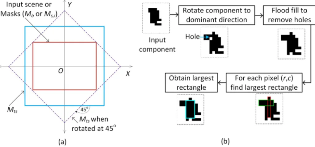
3.4.1 Generate Sub-masks Each sub-mask Ms,i is gener-ated by rotating it to a dominant direction of linesφi with re-spect to the centre of the mask. However, this rotation will cause some parts of the input scene being uncovered by the ro-tated mask. In order to cover the whole scene, a temporary sub-maskMtsis used. It is a square mask with each side equalling tohbt=wbt=

√

2 max(hb, wb). Mtscovers the whole scene (i.e.,MborMs,i), even whenMtsis rotated at any rotation an-gle. Figure 4(a) shows that whenMtsis rotated at45◦it covers the whole scene area.

Consequently,Mtsis rotated, instead ofMs,i, at each dominant angle{φi}to produce a temporary sub-maskMts,i. For exam-ple, fori= 1Figure 3(f) showsMts,1 when rotated at the first dominant direction (φ1= 173.6◦). The mask is shown for vi-sualisation only and cropped to fit the figure. After rotation, the corresponding height value in each pixel location ofMts,1is as-signed from the non-ground point set. Gradients are then calcu-lated in along and across the dominant direction. Considering the error in the supplied point cloud data a thresholdTp= 0.15 m is applied to convert each gradient image into a binary mask. Let these two gradient (binary) images beFx,1andFy,1shown in Figure 3(g)-(h). Basically,Fx,1 represents planes where the height (ideally) remains constant alongφ1but changes alongϕ1.

(4)

Figure 3. Proposed mask generation from a sample scene: (a) aerial image, (b) non-ground points, (c) all image lines (red for ground and cyan for non-ground lines), (d) long lines in eight histogram bins are shown in different colours (lines are at least 3 m in length),

(e) lines in two bins (cyan and yellow) for which two actual dominant directions are estimated (red line shows a non-dominant direction), (f) temporary sub-maskMts,irotated at the first dominant direction (φ1= 173.6◦), (g) gradient imageFx,1, (h) gradient

imageFy,1, (i) flat areasMf,1, (j) sloppy areasMx,1alongφ1, (k) sloppy areasMy,1acrossφ1, (l) sub-masksMs,1, (m) flat areas

Mf,2, (n) sloppy areasMx,2alongφ2, (o) sloppy areasMy,2acrossφ2, (p) sub-masksMs,2.

Figure 4. (a) Generation of the sub-mask – defining building maskMb, sub-maskMs,iand temporary sub-maskMts.MbandMs,i have the same size as the input scene, (b) Steps to find the largest rectangle within a component.

Fy,1 represents planes where the height remains constant along

ϕ1but changes alongφ1. Both of them also contain the flat sur-faces, as shown within pink coloured rectangles in Figure

3(g)-(h), where the height (ideally) remain constant in all directions.

Fx,1andFy,1are then converted back to the original orientation and size. In addition, occasional small holes, which may exist due

(5)

to height jumps between planes or noise in the data, inFx,1and

Fy,1 are filled and small isolated components (maximum 1 m2, i.e., 16 pixels) are removed. Simple binary operations (AND, OR, SUBTRACTION, etc.) are applied to separate the flat areas from

Fx,1andFy,1. Let these three binary images beMx,1(after flat areas are removed fromFx,1),My,1(after flat areas are removed fromFy,1) andMf,1 (contains all flat areas). Figures 3(i)-(k) show all these three images. One of the areas in the flat image is a cuboid shaped vegetation with a flat top (shown within orange coloured rectangle in Figure 3(i)). Figure 3(l) showsMs,1which is simply the result of the OR operation amongMx,1,My,1and

Mf,1.

Figures 3(m)-(p) show all the three images and the sub-mask for

φ2= 124.3◦. Since,φ2is not a principal direction of buildings, but one of the dominant angles for non-ground lines, the building area is mostly missed in the sub-mask. However, as expected the flat areas, as shown Figure 3(m), are clearly captured. While

Mx,2 does not contain any considerable area, My,2 contains a part of the vegetation (shown within orange coloured rectangle in Figure 3(o)).

Figure 3(a) shows two separate vegetation within orange coloured rectangles. As shown in two sub-masks in Figures 3(l) and (p), one of the vegetation is totally removed as it has height variation on its top. The other could not be removed at this point as it is cut into a cuboid with flat top.

3.4.2 Combine Sub-masks Since, it is impossible to distin-guish individual components in eachMts,i (at dominant direc-tionφi), the three binary images (Mx,i,My,iandMf,i) are used to combine the sub-masks.

For each binary image, a connected component analysis is con-ducted. For each connected component the MATLAB function

bwconncompprovides its area, convex hull and pixel locations. Considering that the minimum dimension (length or width) of a single isolated building isWm= 3m, any component which is smaller thanAm= 9m2is subject to a dimensionality test in or-der to keep the component as a part of a big building. The largest rectangleRlcontaining only the pixels of the component is ob-tained. Both dimensions ofRlshould be at leastlm= 1m in the test. This means the minimum width or length of a plane is 1 m. If a component fails this test it is removed as a vegetation. Figure 4(b) shows the steps for finding Rl for the component shown within orange coloured rectangle in Figure 3(i). The out-put for each step is shown at the bottom of that step. First, the component is rotated to its corresponding dominant directionφi (i= 1for this component). For rotation, the procedure described in Section 3.4.1 is followed. Second, the rotated component is flood filled (using the MATLAB functionimfill) in order to re-move any holes that exist due to rotation. Thirdly, for each pixel (r, c) find the height and width of the largest all-black rectan-gle with its upper-left corner at(r, c). Two such rectangles are shown in red and green colours. Finally, from all such rectangles the largest rectangleRl, shown in cyan colour, is obtained. Thereafter, the overlap between any two components at any dom-inant directions are examined. There may be a small thin overlap along the edges between neighboring components due to the digi-tisation effect. Moreover, when many dominant directions exist in a given scene, some building planes can be captured in more than one dominant direction. In some cases, even neighbouring (near) parallel planes can be found partially or fully merged in

some dominant directions. For making sure that each connected component represents one or more building planes and no two components represent the same plane, the following procedure is followed in order to select, remove and/or replace the connected components.

All the connected components ςj, where j≥1, are initially marked as ‘selected’ irrespective of their dominant directions. They are then sorted in descending order of their areas. Start-ing from the largest ‘selected’ component ςm, all components

ςn,k, where k≥1, within the neighbourhood of ςmare found. This neighbourhood search is simply accomplished considering the intersection of convex hulls. Now, for each neighbourςn,kits percentage of overlap withςmis estimated. If there is a major overlap (more than50%), it is tested that the overlap area has at least one component which is at least 1 m2_{in area (}

Test1). This test ensures that thin overlaps along the edges of neighbouring planes does not cause any wrong decision. IfTest 1 is passed, large components from the non-overlap area of thisςn,kare ob-tained separately and marked ‘selected’ (Test2). To find a large area, again the largest rectangleRlcontaining only the pixels of the component is obtained. Both dimensions ofRlshould be at leastlm= 1 m in the test. IfTest1 is failed, a slightly flexi-ble condition is applied to still consider the non-overlap area of

ςn,kif it has large components (Test3). These large components should be at least 1 m2in area. If at least one large area is found (Test2 or 3 is passed), the correspondingςn,k is marked as ‘re-placed’. If no such large area is found (Test2 or 3 is failed), then

ςn,k is marked as ‘removed’. Note that in the above procedure, when necessary, the connected component analysis is conducted on the overlap and non-overlap areas separately for eachςn,k. For the sixth largest componentςm,6, which is Component 1 in

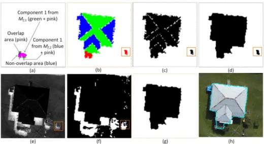
Mf,1 (see Figure 3(i)), two components are found in its neigh-bourhood:ςn,1, which is Component 2 inMx,1(see Figure 3(j)), and (ςn,2), which is Component 1 inMf,2(see Figure 3(m)). No overlap exists betweenςn,1andςm,6. Figure 5(a) shows the over-lap area betweenςm,6andςn,2and the non-overlap area forςn,2. Since the overlap area is93% and 5.4 m2 in area (pink area),

Test1 is passed. Test2 is conducted but is failed, because six components (blue areas), each less than 1 m2in area, are found. Consequently,ςn,2is marked as ‘removed’.

Figure 5(b) shows individual surviving components fromMx,i,

My,iandMf,i in green, blue and red colours respectively. All these components which still remain ‘selected’ are combined (bi-nary OR operation) to find the building mask. The combined mask is shown in Figure 5(c). Thereafter, the combined mask is flood filled in order to fill any holes that may exist due to digiti-sation effect and slope discontinuity between planes. A morpho-logical opening filter is applied with a square structural element of 1 m2in size to reduce the zigzag pattern around the building boundary. Figure 5(d) shows the binary mask, where there are two candidate buildings exist.

3.5 Finalise Buildings

As shown in Figures 5(c-d) within the orange coloured rectan-gle, a small but dense vegetation could not be removed due to its planar top. For such a dense and planar vegetation the laser ray cannot penetrate through to the trunk or the ground and, thus, the vegetation show low gradient values and eventually it remains as a building in the building mask. However, such vegetation (false buildings) are rare and small in size.

(6)

Figure 5. Combining components of sub-masks: (a) analysing overlap and non-overlap areas between components, (b) coloured mask, (c) binary mask, (d) candidate buildings, (e) normalised difference vegetation index (NDVI) for sample scene in Figure 1(a), (f) NDVI

mask, (g) final building mask and (h) final building boundaries. In order to remove such vegetation, a simple analysis with

normalised difference vegetation index (NDVI) is followed (Awrangjeb et al., 2010) for candidate buildings smaller than 10 m2. Figure 5(e) shows the NDVI image for the sample scene in Figure 1(a). Figure 5(b) shows the binary NDVI mask after application of the NDVI threshold (see (Awrangjeb et al., 2010) for details). If within a candidate building the mean NDVI ex-ceeds the NDVI threshold then this candidate is removed as a vegetation. At last, small (say, 1 m2in area) isolated buildings are removed. Figure 5(g) shows the final building mask and Fig-ure 5(h) shows the building boundary. The boundary extraction procedure in (Awrangjeb and Fraser, 2014) is followed.

4. PERFORMANCE STUDY

In the performance study conducted to assess the proposed ap-proach, three data sets from two different areas were employed. The objective evaluation followed a previously proposed au-tomatic and threshold-free evaluation system (Awrangjeb and Fraser, 2012).

The planimetric accuracy has been measured in both object and image space. In object-based evaluation the number of buildings has been considered – whether a given building in the reference set is present in the detection set. Five indices are used for object-based evaluation: completenessCm, correctnessCr, qualityQl, detection cross-lapCrd(over-segmentation error) and reference cross-lapCrr(under-segmentation error) rates. In pixel-based image space evaluation the number of pixels has been considered – whether a pixel in a reference building is present in any of the detected buildings. A total of 5 pixel-based evaluation indices are used, these being: completenessCmp, correctnessCrp, quality

Qlp, branching factorBf and miss factorMf. In addition, root-mean-square-error (RMSE) has been used to estimate the geomet-ric error between reference and detected building boundaries. For definitions and formula see (Awrangjeb et al., 2010).

4.1 Data Sets

The test data sets cover two urban areas in Queensland, Australia: Aitkenvale (AV) and Hervey Bay (HB). The AV area comprises two scenes. The first scene (AV1) covers an area of 108 m×80

m and contains 63 buildings. The second (AV2) covers an area of 66 m×52 m and contains 5 buildings. The HB data set has one scene and covers 108 m×104 m and contains 25 buildings. All three data sets contain mostly residential buildings and they can be characterised as urban with medium housing density and moderate tree coverage that partially covers buildings. AV2 com-prises more vegetation and small buildings than AV1 and HB. In terms of topography, AV is flat while HB is moderately hilly. For both AV and HB data sets, LIDAR coverage comprises first-pulse returns with a point density of 35 and 13 points/m2, respec-tively, and the image data comprise multispectral orthoimagery with resolutions of 0.05 m and 0.2 m, respectively. Bare-earth DTMs of 1 m horizontal resolution cover both areas.

Two dimensional reference data sets were created by monoscopic image measurement using the Barista software (Barista, 2011). All visible buildings were digitised as polygons irrespective of their size. The reference data included garden sheds, garages, etc. These were sometimes as small as 5 m2in area.

4.2 Parameter Setting

The proposed building detection uses a number of parameters. Majority of them have been adopted from the existing research works. For example, the height thresholdhc= 1m, the mask resolutionrb= 0.25m and the smallest building size 10 m2are from (Awrangjeb and Fraser, 2014); the minimum building width

Wm= 3m is from (Rottensteiner et al., 2005); and maximum point-to-point distancedmis from (Awrangjeb et al., 2010). The gradient thresholdTp= 0.15m is similar to the normal distance from point to plane (Awrangjeb and Fraser, 2014). Since, there is a height error in the supplied LIDAR data, all points at the same height usually do not have the same recorded height value. This error is sometimes in the range of±0.30m. Thus, the use ofTp= 0.15m is even lower than the estimated error. The an-gle threshold between successive bins of linesθd= ₃₂πradis also smaller than existing threshold (₁₆πrad) used for the principal di-rections of buildings (Awrangjeb, 2016). A small value ofθdwill allow to find more dominant directions of lines. However, in a given scene if it is observed that the number of dominant direc-tions could be low,θd=₁₆πradcan be used. The use of 1 m2

(7)

Figure 6. Building detection in (a-b) Aitkenvale (AV1 & AV2) and (c) Hervey Bay (HB) data sets, (d-h) some difficult areas in AV2 data set [marked with letters in (b)]. Cyan coloured polygons indicate detected buildings and red coloured polygons show missing

buildings. threshold as the smallest plane or building area and morphologi-cal filter size is also justified, since for the given the point density buildings and sheds smaller than 5 m2are hard to detect.

4.3 Experimental Results

Figures 6(a-c) show building detection results visually. As can be seen, all buildings in AV1 and HB data sets were correctly detected. However, many of the buildings were found merged (over-segmentation) with neighbouring buildings due to very lit-tle or no gaps between buildings in these two scenes. Some such errors are shown within orange coloured dotted rectangles in Fig-ures 6(a) and (c). This merging error was observed less in number in AV2 data set where most of the buildings are well separated. But because of the occlusion and shadow problems, caused by dense vegetation, some small buildings could not be detected in AV2 data set.

Table 1 shows the object-based evaluation results on the test data sets. As can be seen, completeness, correctness and quality val-ues for both AV1 and HB data sets are at the maximum (100%). However, the detection cross-lap rate (over-segmentation error) was high in these data set. In contrast, over-segmentation error was lower in AV2 data set, which is a quite complex data set and where some small buildings were missed due to shadow and se-vere occlusion. In this data set, completeness, correctness and quality values went up for buildings larger than 10 m2in area. Figures 6(d-h) describe some difficult areas from AV2 data set. These areas are marked by letters in Figure 6(b). Some buildings, indicated within red coloured polygons, could not be detected mainly because of small in size, high occlusion and shadow. Small buildings do not have enough points reflected from their roofs to capture them into the proposed gradient-based building mask. Occlusion by trees offers high gradient measurements and,

Table 1. Object-based evaluation results in AV1 - first Aitkenvale, AV2 - second Aitkenvale and HB - Hervey Bay scenes. (Cm= completeness,Cr= correctness,Ql= quality,

Crd= detection cross-lap rate andCrr= reference cross-lap rate in percentage.Cm,10,Cr,10andQl,10are completeness, correctness and quality values for buildings with at least 10 m2

in area.) Data set Cm Cr Ql Crd Crr Cm,10 Cr,10 Ql,10 AV1 100 100 100 33.3 0 100 100 100 AV2 82.8 98 81.4 3.8 3.2 92.3 98 90.6 HB 100 100 100 22.2 9.1 100 100 100 Average 94.3 99.3 93.8 19.8 4.1 97.4 99.3 96.9

Table 2. Pixelbased and geometric evaluation results in AV1 -first Aitkenvale, AV2 - second Aitkenvale and HB - Hervey Bay scenes. (Cmp= completeness,Crp= correctness,Qlp= quality,

Bf = branching factor andMf= miss factor in percentage. RMSE = root-mean-square-error in metre.)

Data set Cmp Crp Qlp Bf Mf RM SE

AV1 92.8 97.2 90.4 2.9 7.7 0.63

AV2 84.2 96.8 81.9 3.3 18.7 0.89

HB 95 79.7 76.4 25.5 5.3 0.58

Average 90.7 91.2 82.9 10.6 10.6 0.70

thus, occluded buildings are hard to detect. Shadow increases the average NDVI value within a building area. As a result, candidate buildings exhibiting high NDVI values were removed. Moreover, some of the detected and missing buildings in Figure 6(g) are not only small in size and partially occluded but also of hexagonal sheds with triangular roof planes. The proposed building mask could not capture these small triangular planes well because of high gradient values between small triangular planes and

occlud-ISPRS Annals of the Photogrammetry, Remote Sensing and Spatial Information Sciences, Volume IV-4/W4, 2017 4th International GeoAdvances Workshop, 14–15 October 2017, Safranbolu, Karabuk, Turkey

(8)

ing trees.

Table 2 shows the pixel-based and geometric evaluation results on the test data sets. Pixel-based completeness, correctness and quality values are more than 90% for AV1 data set, and more than 80% for AV2 data set. Nevertheless, the correctness value (hence, its quality value) for HB data set went down below 80% due to high over-segmentation errors, which are shown within an orange coloured dotted rectangles in Figure 6(c). Some de-tection polygons cover not only more than one actual buildings, but also surrounding fence and trees. This is also evident from a high branching factor (25.5%) for HB data set. Since, some small buildings were missed and many buildings could not be completely extracted due to occlusion in AV2 data set, its miss factor is higher (18.7%) than that of AV1 (7.7%) and HB (5.3%) data sets.

In terms of geometric error,RMSEvalue is higher for AV2 data set than for AV1 and HB data sets. Due to partial occlusions in many of the detected buildings in AV2 data set (see detected buildings shown in Figures 6(d)-(h)) they could not be completely extracted. These partially extracted buildings also contributed to the high miss factor for AV2 data set.

4.4 Comparative Results

Earlier the three test data sets were used for performance evalua-tion in (Awrangjeb and Fraser, 2014). In terms of object-based evaluation, (Awrangjeb and Fraser, 2014) performed the same as the proposed method in AV1 and HB data sets. However, in AV2 data set the proposed method outperformed (Awrangjeb and Fraser, 2014). While the completeness and quality values were below 70% by (Awrangjeb and Fraser, 2014), they are above 80% by the proposed method. This is because the proposed method is able to extract many transparent buildings exist in AV2 data set. The pixel-based correctness was also higher by the proposed method.

Despite the high object-based success of the proposed method, it has following limitations. Firstly, its pixel-based accuracy in terms of completeness and quality is slightly lower than that in (Awrangjeb and Fraser, 2014). Secondly, it does not work well with low density point cloud data. The proposed gradient-based mask cannot capture the small roof segments due to a low num-ber of points reflected from roofs. It was tested with point density less than 10 points/m2_{and found ineffective. However, since high} density point cloud data are becoming cheaper and more widely available now-a-days, the application of the proposed method to capture transparent and small buildings would offer a competi-tive alternacompeti-tive, specially where a high object-based performance is required, for example, the detection of buildings in remote country side (e.g., hilly and/or highly vegetated areas) for disaster (e.g., bushfire) management.

5. CONCLUSION

This paper has proposed a new building detection technique from the high density point cloud data and multispectral imagery. The newly proposed building mask is based on the gradient calcu-lation on the height grid obtained at the dominant directions of non-ground image lines. Due to application of the gradient func-tion on the height grid, any vegetafunc-tion with random 3D surface is mostly removed. Thus, buildings become easily identifiable. As the proposed mask uses the non-ground points, it can cap-ture the buildings with transparent roof materials. As a result,

the proposed mask integrates the benefits of two existing masks: the nDSM and the primary mask. Some false candidate build-ings, specially found on planar surfaces of some vegetation, are removed with the application of NDVI from the multispectral im-agery. The experimental results have shown its higher object-based performance than that of an existing building detection technique (Awrangjeb and Fraser, 2014). Moreover, it is capable of detecting small garden sheds, which are sometimes as small as 5 m2in area.

However, the proposed technique has some drawbacks. Its pixel-based accuracy is slightly lower than the existing technique and it does not work with low density point cloud data. The future work includes investigation of more effective building mask that would be more effective, specially with increased pixel-based accuracy and reduced over-segmentation error.

ACKNOWLEDGMENT

The authors would like to thank Ergon Energy (www.ergon.com.au) for providing the Australian data sets. Dr. Awrangjeb is a recipient of the Discovery Early Career Researcher Award by the Australian Research Council (project number DE120101778).

REFERENCES

Awrangjeb, M., 2016. Using point cloud data to identify, trace, and regularize the outlines of buildings.International Journal of Remote Sensing37(3), pp. 551–579.

Awrangjeb, M. and Fraser, C. S., 2012. An automatic and threshold-free performance evaluation system for building ex-traction techniques from airborneLIDARdata. IEEE Journal of Selected Topics in Applied Earth Observations and Remote Sens-ing7(10), pp. 4184–4198.

Awrangjeb, M. and Fraser, C. S., 2014. Automatic segmenta-tion of rawLIDARdata for extraction of building roofs. Remote Sensing6(5), pp. 3716–3751.

Awrangjeb, M., Ravanbakhsh, M. and Fraser, C. S., 2010. Au-tomatic detection of residential buildings usingLIDARdata and multispectral imagery. ISPRS Journal of Photogrammetry and Remote Sensing65(5), pp. 457–467.

Awrangjeb, M., Zhang, C. and Fraser, C. S., 2012. Building de-tection in complex scenes thorough effective separation of build-ings from trees. Photogrammetric Engineering & Remote Sens-ing78(7), pp. 729–745.

Barista, 2011. The barista software.

Habib, A. F., Zhai, R. and Changjae, K., 2010. Generation of complex polyhedral building models by integrating stereo-aerial imagery and lidar data. Photogrammetric engineering & remote sensing76(5), pp. 609–623.

Lee, D., Lee, K. and Lee, S., 2008. Fusion of lidar and imagery for reliable building extraction.Photogrammetric Engineering & Remote Sensing74(2), pp. 215–226.

Rottensteiner, F., Trinder, J., Clode, S. and Kubik, K., 2005. Us-ing the dempstershafer method for the fusion ofLIDARdata and multi-spectral images for building detection.Information Fusion

6(4), pp. 283–300.

Sohn, G. and Dowman, I., 2007. Data fusion of high-resolution satellite imagery and lidar data for automatic building extraction.

ISPRS Journal of Photogrammetry and Remote Sensing62(1), pp. 43–63.