W
ORKING
P
APERS IN
E
CONOMICS
No. 15/07
L
IV
O
SLAND AND
I
NGE
T
HORSEN
T
ESTING FOR THE
I
MPACT OF
L
OCAL
S
PATIAL
S
TRUCTURE
C
HARACTERISTICS
ON
H
OUSE
P
RICES
D
epartment of
E
conomics
________________________
Testing for the impact of local spatial structure characteristics on
house prices
∗Liv Osland and Inge Thorsen†
December 6, 2007
Abstract
The starting point of this paper is a hedonic regression model where house prices are explained as a result of urban attraction and the accessibility to job opportunities in the region. We introduce the hypothesis that households in addition value accessibility to job opportunities in the neighborhood, and study if and how this is reflected in house prices. We propose several measures of local labor market characteristics, and test for the impact on house prices. The alternative measures do not add considerably to the explanatory power. Still, some characteristics contribute significantly, and affect the strength and interpretation of the relationship between local labor market conditions and house prices.
JEL-classification: R21, R31
1
Introduction
In Osland and Thorsen (2008) spatial variation in housing prices were explained to result from an urban attraction and a labor market accessibility effect. Those effects were represented by traveling time from the cbd, and a gravity based measure of labor market accessibility in a hedonic modeling framework. Based on data from the southern parts of Rogaland County in the south west of Norway we found that such spatial characteristics added considerably to the explanatory power in an approach that also accounted for several house-specific attributes in
∗
We would lik to thank Roger Bivand for helpful suggestions.
†
a relatively macroscopical description of the geography. In this paper we test for the possible impact of polycentric tendencies and local characteristics which are not represented by the two globally defined measures of spatial structure.
The empirical results in Osland and Thorsen (2008) refer to a regional rather than an urban context, covering a connected labor and housing market area rather than just an urban area. The macroscopical perspective is reflected by the fact that the geography is subdivided into zones that extend over a relatively large area, and the fact that we consider interzonal rather than intrazonal variations in housing prices. At least in such a macroscopical perspective it can be argued that labour market accessibility and potential commuting distances are of vital importance for how readily saleable a house is, and what price that is achieved.
The idea that the polycentric character of the labor market matters in explanation of housing prices is of course reflected in the literature, see for instance Dubin and Sung (1987), Heikkila et al. (1989), Richardson et al. (1990), Waddell et al. (1993). Those contributions emphasize the importance of including the distance to secondary employment centers, while for instance Adair et al. (2000) introduced a gravity based measure of transport accessibility in a study of the Belfast urban area. As pointed out by McMillen (2004) empirical studies are not unambiguously consistent with standard urban theory, suggesting that both the price of a unit of housing and the population density should be relatively high in and near subcenters. Heikkila et al. (1989) and Richardson et al. (1990) are examples of studies confirming standard theoretical hypotheses, while McMillen (2003) and McMillen (2004) present evidence that proximity to Chicago’s subcenters is not valued highly in the residential market.
Our study applies for a relatively transparent central place system with a dominating city center rather than a complex metropolitan area, and we consider several possibly relevant local structure characteristics, rather than just the presence of subcenters. In general, many authors account for spatial attributes that affect housing prices only in a small area. Heikkila et al. (1989) distinguish between macro-and microlocational effects, and implicitly introduce the im-pact originating from the multipurpose nature of household spatial interaction. Households also value access to other activities than job opportunities. Li and Brown (1980) classify activi-ties relative to three categories of attributes: aesthetic attributes, pollution sources and service facilities.
Due to data restrictions we are not able to account for a wide range of local attributes and activities. More spatially disaggregated data on local attributes would require a massive effort on data collection. In this paper we primarily focus on the impact of the location relative to labor market opportunities rather than a set of local-specific amenities. Considering our macroscopical perspective of the geography a high degree of residential interzonal homogeneity can be expected for many amenities, like for instance the view, the neighborhood quality, or the distance to nursery school. Many attributes of this kind are reasonably equally present in most of the (postal delivery) zones that we consider. We will of course account for the effect of some basic residence-specific attributes (internal living area, lot size, age of building etc.), but we ignore the impact of intrazonal local-specific amenities and services. Similarly, we ignore the possible impact on house prices of systematic variation in zonal socioeconomic characteristics. The spatial structure characteristics we introduce are primarily motivated from hypotheses of spatial labor market interaction.
The lack of information on intrazonal location-specific attributes reduces the potential ex-planatory power of our estimation. To some degree the effect of the omitted variables might for instance be represented by location-specific dummy variables. This is not, however, a recom-mended procedure if focus is primarily on explaining and predicting spatial variation in housing prices. Our macroscopical approach means that we focus on general effects rather than on obtaining a highest possible explanatory power for our study area.
In Section 2 we present the region and our data, while the modeling framework is introduced in Section 3. Alternative measures of local spatial structure are proposed in Section 4.5. Section 5 offers results based on the proposed measures, and results based on semi-parametric approaches are evaluated in Section 6. Finally, some concluding remarks are given in Section 7.
2
The region and the data
The study area in this paper is the southern parts of Rogaland, which is the southernmost county in Western Norway. There are 13 municipalities in the region, and each municipality is divided into postal delivery zones. All in all the region is divided into 98 (postal delivery) zones, as indicated in Figure 1. As an indicator of (commuting) distances, there is 79 km from the center of Stavanger to Egersund in the south. Stavanger is the dominating city in the region,
with about 115000 inhabitants. The region is described in more detail in Osland et al. (2005), and is very appropriate for studies of the relationship between spatial labor market interaction and the housing market. This is due to the fact that it is an integrated and autonomous region; the landscape is fairly homogeneous and the topographical barriers protect from disturbances in other regions, rather than causing spatial submarkets and disconnections in the intraregional transportation network. The region is more or less like an island with one dominating city, and a tendency of an increasing rural profile as the distance increases from this city center.
Stavanger Rennesøy Sola Randaberg Sandnes Klepp Hå Time Gjesdal Bjerkreim Eigersund Lund Sokndal 1 2 3 4 41 5 46 45 47 48 49 50 61 63 53 60 51 52 62 54 55 72 71 73 70 69 56 84 82 83 74 78 76 75 77 81 80 79 88 87 86 89 85 91 90 99 98 95 96 97 94 92 93 43 38 6 40 39 87 9 10 20 15 17 13 11 12 14 21 18 16 19 24 26 22 27 23 25 28 30 29 34 36 31 35 37 44 33 32 58 59 57 67 66 65 64 68 42
Figure 1: The division of the region into municipalities and zones
houses in the period from 1997 through the first half of 2001. Our sample of 2788 property transactions represents approximately 50% of the total number of transactions of privately owned single-family houses in the region during the relevant period. The transactions data on the freeholder dwellings have been provided for us from two sources: the national land register in Norway and Statistics Norway. For more details on those data, and descriptive housing market statistics for separate parts of the region, see Osland et al. (2005).
The division of the region into zones corresponds to the most detailed level of information which is officially available on residential and work location of each individual worker within the region. This information is based on the Employer-Employee register, and provided for us by Statistics Norway.
The matrices of Euclidean distances and traveling times were prepared for us by the Nor-wegian Mapping Authority, who have at their disposal all the required information on the road network and the spatial residential pattern. The calculations were based on the specification of the road network into separate links, with known distances and speed limits, and it is ac-counted for the fact that actual speed depends on road category. Information of speed limits and road categories is converted into travelling times through instructions (adjustment factors for specific road categories) worked out by the Institute of Transport Economics. The center of each (postal delivery) zone is found through detailed information on residential densities and the road network. Finally, the matrices of distances and traveling times are constructed from a shortest route algorithm.
3
The modeling framework
We consider model formulations which distinguish between two categories of attributes. One category is the physical attributes of the specific dwelling, the other is related to spatial structure characteristics and the accessibility to labor market opportunities. In a general form the hedonic price equation can be written as follows:
Pit=f(zsit, zlit) (1)
Pit= the price of housei in yeart
zsit= value of dwelling-specific structural attributesfor houseiin yeart;s= 1, ...S,i= 1, ...n
zlit= value of location-specific attributel for house iin yeart;l= 1, ...L,i= 1, ...n
Table 1 offers a list of non-spatial dwelling-specific attributes incorporated in our modeling framework.
Table 1: List of non-spatial dwelling-specific variables
Variable Operational definition
REALPRICE selling price deflated by the consumer price index, base year is 1998
AGE age of building
LIVAREA living area measured in square meters
LOT lot-size measured in square meters
GARAGE dummy variable indicating presence of garage
NUMBTOIL number of toilets in the building
REBUILD dummy variable indicating whether the building has been rebuilt/renovated
In addition to the dwelling-specific attributes we introduce the variable RURLOT into our regression model specifications. This variable is based on a stratification of the geography into rural and urban areas. The rural areas include four municipalities, see Osland et al. (2005) for details and criteria. RURLOT is defined to be the product of the dummy variable representing rural areas and the variable LOT, defined in Table 1. Osland et al. (2007) found that this spatial characteristic variable increased the explanatory power of the model significantly.
Osland et al. (2007) used the same data set that is considered in this paper to study the relationship between house prices and the traveling time from the cbd. Based on explanatory power in combination with pragmatic, theoretical, econometric, and interpretational arguments, they recommended that the relationship is represented by a power function specification
supple-mented by a quadratic term. Let dij represent the traveling time between the two zones iand
j. Traveling time then enters in the regression equation through the following expression:
h(dij) =dβij·((dij)2)βq (2)
According to the idea of a trade-off between housing prices and commuting costs, Osland and Thorsen (2008) introduced a gravity based measure of labor market accessibility that captures
the fact that job opportunities are not solely concentrated to the cbd. In this Hansen type (Hansen 1959) of accessibility measure traveling time appears through a negative exponential
function. Letσ <0 be the weight attached to traveling time, and γ the parameter attached to
the number of job opportunities,Dk. The accessibility measure,Sj, is then defined as follows:
Sj =
w
X
k=1
Dγkexp(σdjk) (3)
Here,Dkrepresents the number of jobs (employment opportunities) in destination (zone) k.
The measure Sj is based on the principle that the accessibility of a destination is a decreasing
function of relative distance to other potential destinations, where each destination is weighted by its size, or in other words the number of opportunities available at the specific location. Hence, it can be interpreted as an opportunity density function, introduced to account for the possibility that the relevant kind of spatial pull originates from several destination opportunities. The basic hypothesis underlying the introduction of the measure is that workers prefer a location with favorable job opportunities within a reasonable distance from their residential site. Hence, labor market accessibility influences the number of households bidding for a house that is for sale, explaining spatial variation in housing prices. The Appendix offers estimates of the relative
labor market accessibility of all the zones in our study, defined by Sj
1 98
P98
j=1Sj
.
In this paper our “Basic Model”(BM), incorporates both traveling time from the cbd, through Equation (2), and the gravity based labor market accessibility measure (ACCESSIBILITY) through Sj:
logPit = β0+β1log LOTi+β2(RUR log LOT)i+β3log AGEi+β4(REBUILD log AGE)i+
+β5GARAGEi+β6log LIVAREAi+β7log NUMBTOILi+βlog TIMECBDi+
+βq(log TIMECBDi)2+β8log ACCESSIBILITYi+
01 X
t=97
βtYEARDUMit+it (4)
Here, it is the error of disturbance for a specific observation. The model formulation BM is
4
Alternative local spatial structure characteristics
In this paper we test for the possibility that labour market accessibility should be defined at two separate spatial levels of aggregation. The motivation for this test springs out from the hypoth-esis that residential location choices can be considered as the result of a hierarchical, two-step, decision process. As a first step of such a decision process the households determine what parts (municipalities) of the region that is relevant in their search for a house. Residential loca-tion preferences can for example in general be due to environmental condiloca-tions, localoca-tion-specific amenities, public services, friendships and family relations, or simply preferences imprinted from childhood experiences. In this first, macroscopical, step of the decision process, labour market considerations are important, since households, ceteris paribus, prefer a location with favorable job opportunities within a reasonable distance from their residential site. For a related problem Anas et al. (1998) argue that “... two worker households have to compromise between loca-tions convenient to a job, frequent job changes and substantial moving costs cause people to choose locations convenient to an expected array of future jobs rather than just their current job ...”. This perspective further calls for a regional measure of spatial structure, and our rather macroscopic, spatially aggregated, description of the geography is reasonable. The macroscopic perspective especially applies for the most peripheral parts of the region, and is implicitly based on an assumption of a relatively high degree of interzonal homogeneity, where most activities can be performed within each zone.
The second step of the decision process concerns the choice of a residential site within the relevant search area. Any location within this area represents an acceptable combination of job search and realisation of residential site preferences. This does of course not mean, however, that all location alternatives within the area are evaluated to be equivalent. The evaluations are influenced by a multitude of attributes, and individual households do not put the same weight on different attributes. Due to data restrictions we have of course no chance to capture this heterogeneity in preferences and location pattern of attributes. Our ambition is to test for the possible impact from spatial structure and labour market characteristics that are not captured
through the accessibility measure Sj. We discuss the possibility that local variation in spatial
structure characteristics influences housing prices also in a data set corresponding to a relatively macroscopical description of the geography. Such characteristics might systematically affect
individual evaluations, and the willingness-to-pay for a house that is for sale. In the subsections to follow we are specific on the formulation of local accessibility measures.
4.1 Subcenters
Despite the fact that both employment and population are strongly concentrated to Stavanger and adjacent municipalities, some other regional subcenters can be identified. Guiliano and Small (1991) focus on how subcenters typically develop as a conflict between agglomeration forces and congestion effects, and they discuss empirical criteria for identifying subcenters. Both McDonald (1987) and Guiliano and Small (1991) argue that employment, not population, is the key to understand the formation of centers, and the usual definition of a subcenter is a set of contiguous tracts with significantly higher employment densities than surrounding areas (McMillen 2004). Guiliano and Small (1991) propose criteria based on a specific density cutoff of employees per acre and a minimum total employment. Others, for instance McDonald (1987) and McMillen (2001), use statistically based criteria to identify subcenters from estimated employment density functions. The mentioned studies refer to large and complex metropolitan areas, like Chicago (McMillen 2002, 2004) and Los Angeles (Guiliano and Small 1991). Our study area is more transparent, and subcenters can be identified from prior knowledge of the geography.
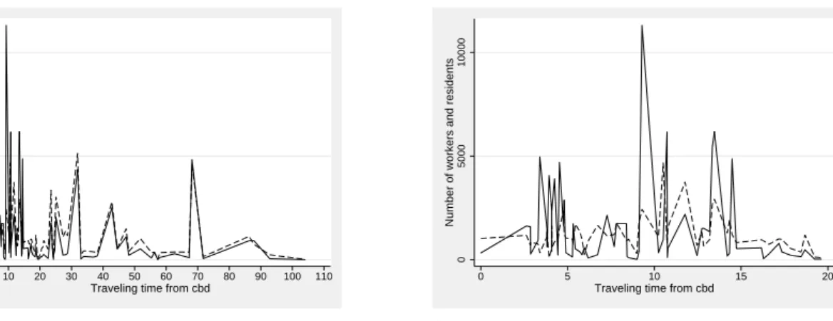
The left part of Figure 2 illustrates how employment and population are distributed across our study area, with travel time from the peak of the Stavanger cbd represented on the hori-zontal axis. The figure indicates that two marked subcenters can be identified outside the most central parts of the region. Those are the centers of the municipalities Time and Eigersund, respectively, and they are represented by two marked peaks in employment densities, in a trav-eling time by car of about 32 and 68 minutes from the regional center. Notice also from the left part of Figure 2 that the spatial distribution of workers (population) has a marked peak in those two subcenters, where the number of jobs is approximately balanced to the number of workers. Based on information of commuting flows, Statistics Norway categorizes the two zones as subregional centers in the geography. The right part of the figure illustrates that jobs are spatially considerably less balanced to workers in the central part of the region, where the subdivision of the geography into zones is more disaggregate.
formu-0
5000
10000
Number of workers and residents
0 10 20 30 40 50 60 70 80 90 100 110
Traveling time from cbd a) The entire region
0
5000
10000
Number of workers and residents
0 5 10 15 20
Traveling time from cbd b) The central area of the region
Figure 2: The spatial distribution of jobs and workers. The solid lines represent the number of jobs, while the dashed line represents the number of workers residing at alternative locations.
lation: SUBi =
1 if the house is located in subcenter i;i= 1,2
0 otherwise
In addition, a natural hypothesis is that house prices vary systematically with distance from those subcenters, even in a model formulation where regional labor market accessibility is accounted for. Is here a similar attraction effect that was identified for the Stavanger cbd area? Is it possible that households, like firms, are attracted to centers through some kind of agglomeration effects, for instance related to the probability of having matching neighbors? Such hypothesis and questions motivate our modeling alternative LM1:
LM1: The basic model (BM) extended by two dummy variables (SUB1 and SUB2)
repre-senting the presence of the two subcenters, and corresponding variables (SUB1DIST and SUB2DIST) representing traveling times within a specific cutoff value of 20 minutes from the subcenters SUB1 (Bryne) and SUB2 (Egersund).
The choice of a cutoff value of 20 minutes is a result of experiments with several alterna-tive values, and it represents the distance where the subcenter has no longer an influence on house prices. Without finding significant results to be reported we have also experimented by incorporating several alternative subcenters into our model. One obvious choice is the center of Sandnes. Our results indicate, however, that this subcenter is adequately represented by the spatially defined variables in the basic model, as an integrated part of the Stavanger urban area. Another hypothesis is that housing prices is systematically higher nearby the administrative
center in a municipality than elsewhere. This hypothesis can be motivated from the possibility that households on average find it attractive and convenient to reside close to services offered by local authorities. A modeling alternative corresponding to this hypothesis is:
LM2: The basic model (BM) extended by a dummy variable (ADMCENTER) representing the
administrative center of a municipality.
The dummy variable is defined by
ADMCENTER =
1 if zone is the administrative center of its municipality
0 otherwise
4.2 Local opportunities of employment
It can be argued that the specification of spatial structure in our basic model do not adequately reflect complex systematic multipurpose decisions within households. Two-worker households might, for instance, prefer residential locations with favorable job opportunities in the close neighborhood. Short journeys-to-work facilitate the logistics of running the household, and potentially reduces transport costs, for instance by reducing the need for disposing two cars. One hypothesis is that such effects can be represented by a simple cumulative opportunities measure of accessibility, for instance defined by the number of job opportunities reached within a travel time by car of 5 minutes (see for instance Yinger (1979) and Handy and Niemeier (1997)). Ideally, the measure should reflect the probability of receiving relevant job offers, capturing both the labor market turnover (vacancies) and the diversity of job opportunities. The number of jobs within an area represents, of course, only a rough proxy variable of the relevant labor market situation in alternative areas, but we doubt that the payoff in form of more significant results is reasonably related to the considerable amount of data collection required to study the matters in more detail.
Another data-driven simplifying assumption is related to our aggregate subdivision of the geography into rather wide-spreading zones. This complicates a confident specification of em-ployment rings corresponding to a specific traveling times from alternative locations. As an alternative measure of the local labor market situation we have instead used the intrazonal employment:
LM3: The basic model (BM) extended by a variable (JOBS) representing the number of jobs within the zone.
4.3 Population density
Our search for relevant local measures of spatial structure is primarily based on considerations of spatial labor market behavior. The distinction between local and regional accessibility can, however, also be motivated from hypotheses on other kinds of spatial interaction than com-muting. Handy (1993) studies spatial differences in average shopping distances and shopping frequencies within a gravity based modeling framework where accessibility is defined at a local and a regional level. Communities with low local but high regional accessibility are found to induce the most amount of automobile travel. A natural hypothesis is that such differences in transaction costs are reflected in house prices. Our data do not allow for incorporating explicitly the spatial distribution of shopping facilities, however. Similarly, we are not able to account for the impact of individual preferences and interdependencies, and effects of proximity to schools, kindergartens, and specific amenities. A reasonable hypothesis is that the presence of relevant local attributes is positively related to the population density. The population density might in principle be represented by the number of workers residing within rings of a specific traveling time from a location. Once again, however, the use of such a simple measure is complicated by our aggregate subdivision of the geography into zones. Instead, we test the hypothesis that the population within a zone affects the housing prices. We assume that population is represented by the number of workers residing within a zone.
LM4: The basic model (BM) extended by a variable (POPULATION) measuring the number
of workers residing in a zone.
4.4 The number of jobs per worker
We have argued that the attractiveness of a location for residential purposes depends on the probability of receiving relevant job offers locally. Due to distance deterrence effects in the job-search procedure and to costs related to the journey-to-work it further can be argued that this probability depends positively on the number of jobs per inhabitant within a zone. This hypothesis is examined through the following model formulation
LM5: The basic model (BM) extended by a variable measuring the number of jobs per worker (BALANCE) residing within a zone.
4.5 Relative local labor market accessibility
As pointed out by Guiliano and Small (1991) local subcenters can also be identified through gravity based measures of accessibility. Analogously, we characterize the labor market position of a zone through a measure of relative accessibility. Let
g(i, j) =
1 if zoneiand zonej have a common boundary
0 otherwise
n(i) = # zones with a boundary common to zone i
and
Z(j) = [j:g(i, j) = 1]
whereZ(j) = the set of zones with a boundary common to zonei
The relative accessibility of a zone is then defined by:
RELACCi= Si 1 n(i) P j∈Z(j)Sj (5)
where Si is the labor market accessibility of a zone, as defined by Equation (3). A high value
of this measure means that the corresponding zone has a high local labor market accessibility. LM5 is introduced to test whether this measure contributes positively to explain variation in housing prices:
LM6: The basic model (BM) extended by the variable RELACCi, reflecting local variations in
labor market accessibility.
Based on data-driven experiments we also introduce the hypothesis that this measure of local labor market accessibility is defined relative to specific areas of the geography. The most central parts of the region represent an urban area, including Stavanger as well as lower rank central places and suburban communities in the municipalities surrounding Stavanger (Stavanger, Sola, Randaberg, and Sandnes, see the map in Figure 1). The rural area represents four municipalities
(Sokndal, Lund, Bjerkreim, and Gjesdal) in the hinterland in the southern parts of the region, where the ratio of inhabitants to open land is considerably lower than in other municipalities. The remaining zones are neither located in the most urban nor in the most rural parts of the region, and define a semi-urban area. The three subareas are identified through dummy variables, like for instance:
URBAN(i) =
1 if zoneibelongs to the most urban parts of the region
0 otherwise
The variables RURAL(i) and SEMI(i) are similarly defined, and the corresponding areas are
defined byU(i) = [i: URBAN(i) = 1], R(i) = [i: RURAL(i) = 1], and SU(i) = [i: SEMI(i) = 1]. Let
n(U) = # the number of zones within the urban area
The relative local labor market accessibility of zonei within the urban area is defined by:
RELACC(U)i = 1 RELACCi
n(U) P
j∈U(j)RELACCj
·URBAN(i) (6)
RELACC(R)i and RELACC(SU)i are similarly defined as the relative local labor market
acces-sibility of zone iwithin the rural and the semi-urbanized areas, respectively. This specification
complies to the idea that a local measure of labor market accessibility should refer to the loca-tion within a subarea rather than the entire region. The basic hypothesis is that the residential preferences of households might be in favor of a particular kind of area, like an urban area, a rural area, or a semi-urban area, and that high accessibility to job opportunities on average is considered as an attractive location attribute within this area. This suggests that the pa-rameter estimates corresponding to the area-specific accessibility measures are positive. The corresponding model formulation is represented by
LM7: The basic model (BM) extended by variables reflecting local variations in labor market
accessibility within specific subareas of the region.
Finally, we have tested model formulations combining several of the proposed local measures of spatial structure:
LM8: The basic model (BM) extended by several characteristics of local spatial structure.
The alternative local structure characteristics are introduced log-linearly in the corresponding hedonic regression models.
Notice also that our procedure is implicitly based on the assumption of internal spatial price arbitrage in the region, see for instance Jones (2002) for a discussion of spatial arbitrage. This means that implicit prices of specific attributes are assumed to be leveled out through among other things, migration and commuting decisions in a region with a connected, efficient, transportation network. In other words, our approach is based on the assumption of a single competitive market, rather than a set of submarkets with varying implicit prices. The assump-tion of spatial coefficient homogeneity is not without excepassump-tions, however. The variable reflecting local variation in labor market accessibility is assumed to apply for specific subareas in LM7, and the implicit price of lotsize is assumed to differ in rural and non-rural areas. According to our results a lot located in rural areas is not a perfect substitute for a lot located in non-rural areas.
5
Results
In this section we present estimation results based on the alternative model formulations that were proposed in the preceding section. We also search for relevant local characteristics through a data-mining semiparametric approach.
5.1 An empirical evaluation of the alternative model formulations
The analysis to follow is based on the use of pooled cross section data. This explains the introduction of the time-dummies in our models. The advantage of this procedure is that it enables an increase in sample size, and greater variations in the independent variables.
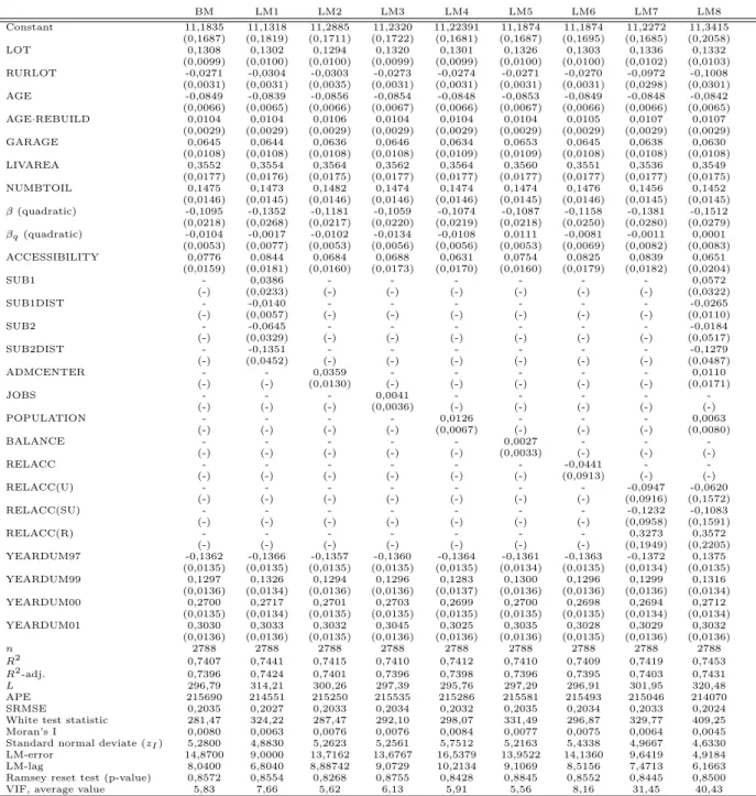
Results from the experiments with measures of the local spatial structure are presented in Table 2. Consider first the results based on LM1. Compared to the basic model (BM) all the measures of explanatory power are improved, but the changes are not very convincing.
Still, the value of the likelihood ratio test statistic is (2·(314,21−296,79) ≈) 34,8, which
significance level. The reported positive loglikelihood values are explained from the fact that the logarithm of house prices defines a function that is very flat for the relevant range of values, with correspondingly small variance (see Osland et al. 2007).
Our results indicate that an attraction effect is present for the two subcenters, analogously to the urban attraction originating from the Stavanger cbd. The partial impact of a location at Bryne is estimated to be positive, but the effect is not significant at the 5% level. The estimated partial effect of a location in Egersund is, on the other hand, significantly negative. In interpreting this result, remind that effects of job concentrations are accounted for through the labor market accessibility measure. It also follows that the position of Egersund as a center in the southern parts of the region is reflected in the parameter estimate corresponding to the variable SUB2DIST.
Notice from Table 2 that the estimated effect of variations in distance is considerably larger for Egersund (SUB2DIST) than for Bryne (SUB1DIST). This is a reasonable result. Bryne is surrounded by smaller centers of a lower rank, while Egersund is a center for a more rural area in a considerably longer distance from the central parts of the region. The housing market in the Bryne area is therefore more influenced by the situation in the cbd of the region. The coefficient related to SUB1DIST reflects a rather marginal effect of variations in distance on housing prices. The estimate implies that the price of a standard house falls by about 118000 NOK (8%) from the center of Bryne to a location 20 minutes from this center, ceteris paribus. For Egersund the estimate implies a corresponding reduction of about 318000 NOK (28%).
As mentioned in Section 4.1 we have also experimented by incorporating several alternative subcenters, without finding significant effects on house prices. It is further clear from the brief literature review in the introduction that our somewhat ambiguous results are according to empirical findings in other studies. McMillen (2004) is an example of a study concluding that proximity to subcenters is not highly valued in the residential market. Suburban trips in this study (Chicago) are less time-consuming than trips to the cbd. McMillen’s argument further is that workers are willing to endure potentially lengthy commutes when they take jobs in a subcenter. This argument is of course less valid for the study area that we consider, but it might still contribute to explain the relatively modest effects on house prices of the presence of subcenters.
Accounting for the presence of subcenters only leads to marginal changes in most of the remaining parameter estimates. The parameters that are relatively most sensitive to the model
extension areβ andβqand the parameter attached to the accessibility measure. If relevant
spa-tial structure characteristics are not accounted for in the model formulation an estimation bias will result. This bias especially appears for other variables representing spatial structure charac-teristics. Notice in particular that the effect of the quadratic term in the function representing distance from the cbd becomes redundant in the case where the presence of relevant subcenters is explicitly taken into account. If spatial structure in general is adequately accounted for in the model formulation, there is no need for a flexible functional representation of traveling time to capture irregularities in the housing price gradient.
According to our estimation results the dummy variable ADMCENTER in general has no significant influence on housing prices in the region, and the introduction of this variable does not lead to a significant increase in explanatory power. We have not, however, included the results based on this general formulation of the model in Table 2. Based on an inspection of residuals we found a tendency that the basic model underpredicts house prices in the 5 most centrally located administrative centers outside Stavanger (the centers of Sola, Randaberg, Sandnes, Bryne, and Gjesdal). As a result of this data-mining procedure we reached a model specification performing better than a general representation of the variable ADMCENTER. This is the model specification underlying LM2 in Table 2. According to the table the variable ADMCENTER contributes significantly to explain spatial variation in house prices, and the
value of the likelihood ratio test statistic is (6,94) exceeds the critical value of a chi square
distribution with 1 degree of freedom at the 5 percent significance level. The choice of the relevant subset of administrative centers is not, however, based on reasonable hypotheses on labor and housing market behavior.
The number of jobs within a zone (JOBS) is not found to influence housing prices signif-icantly, and it does not lead to a significantly improved goodness-of-fit (see the results based on LM3 in Table 2). Still, we cannot jump to the conclusion that the local supply of jobs does not influence housing prices. We can of course not ignore the possibility that the results are due to our specification of the local labor supply. We have carried through experiments with adjustments in this specification, both by restricting the variable to groups of municipalities,
Table 2: Results based on alternative specifications of local spatial structure characteristics BM LM1 LM2 LM3 LM4 LM5 LM6 LM7 LM8 Constant 11,1835 11,1318 11,2885 11,2320 11,22391 11,1874 11,1874 11,2272 11,3415 (0,1687) (0,1819) (0,1711) (0,1722) (0,1681) (0,1687) (0,1695) (0,1685) (0,2058) LOT 0,1308 0,1302 0,1294 0,1320 0,1301 0,1326 0,1303 0,1336 0,1332 (0,0099) (0,0100) (0,0100) (0,0099) (0,0099) (0,0100) (0,0100) (0,0102) (0,0103) RURLOT -0,0271 -0,0304 -0,0303 -0,0273 -0,0274 -0,0271 -0,0270 -0,0972 -0,1008 (0,0031) (0,0031) (0,0035) (0,0031) (0,0031) (0,0031) (0,0031) (0,0298) (0,0301) AGE -0,0849 -0,0839 -0,0856 -0,0854 -0,0848 -0,0853 -0,0849 -0,0848 -0,0842 (0,0066) (0,0065) (0,0066) (0,0067) (0,0066) (0,0067) (0,0066) (0,0066) (0,0065) AGE·REBUILD 0,0104 0,0104 0,0106 0,0104 0,0104 0,0104 0,0105 0,0107 0,0107 (0,0029) (0,0029) (0,0029) (0,0029) (0,0029) (0,0029) (0,0029) (0,0029) (0,0029) GARAGE 0,0645 0,0644 0,0636 0,0646 0,0634 0,0653 0,0645 0,0638 0,0630 (0,0108) (0,0108) (0,0108) (0,0108) (0,0109) (0,0109) (0,0108) (0,0108) (0,0108) LIVAREA 0,3552 0,3554 0,3564 0,3562 0,3564 0,3560 0,3551 0,3536 0,3549 (0,0177) (0,0176) (0,0175) (0,0177) (0,0177) (0,0177) (0,0177) (0,0177) (0,0175) NUMBTOIL 0,1475 0,1473 0,1482 0,1474 0,1474 0,1474 0,1476 0,1456 0,1452 (0,0146) (0,0145) (0,0146) (0,0146) (0,0146) (0,0145) (0,0146) (0,0145) (0,0145) β(quadratic) -0,1095 -0,1352 -0,1181 -0,1059 -0,1074 -0,1087 -0,1158 -0,1381 -0,1512 (0,0218) (0,0268) (0,0217) (0,0220) (0,0219) (0,0218) (0,0250) (0,0280) (0,0279) βq(quadratic) -0,0104 -0,0017 -0,0102 -0,0134 -0,0108 0,0111 -0,0081 -0,0011 0,0001 (0,0053) (0,0077) (0,0053) (0,0056) (0,0056) (0,0053) (0,0069) (0,0082) (0,0083) ACCESSIBILITY 0,0776 0,0844 0,0684 0,0688 0,0631 0,0754 0,0825 0,0839 0,0651 (0,0159) (0,0181) (0,0160) (0,0173) (0,0170) (0,0160) (0,0179) (0,0182) (0,0204) SUB1 - 0,0386 - - - 0,0572 (-) (0,0233) (-) (-) (-) (-) (-) (-) (0,0322) SUB1DIST - -0,0140 - - - -0,0265 (-) (0,0057) (-) (-) (-) (-) (-) (-) (0,0110) SUB2 - -0,0645 - - - -0,0184 (-) (0,0329) (-) (-) (-) (-) (-) (-) (0,0517) SUB2DIST - -0,1351 - - - -0,1279 (-) (0,0452) (-) (-) (-) (-) (-) (-) (0,0487) ADMCENTER - - 0,0359 - - - 0,0110 (-) (-) (0,0130) (-) (-) (-) (-) (-) (0,0171) JOBS - - - 0,0041 - - - - -(-) (-) (-) (0,0036) (-) (-) (-) (-) (-) POPULATION - - - - 0,0126 - - - 0,0063 (-) (-) (-) (-) (0,0067) (-) (-) (-) (0,0080) BALANCE - - - 0,0027 - - -(-) (-) (-) (-) (-) (0,0033) (-) (-) (-) RELACC - - - -0,0441 - -(-) (-) (-) (-) (-) (-) (0,0913) (-) (-) RELACC(U) - - - -0,0947 -0,0620 (-) (-) (-) (-) (-) (-) (-) (0,0916) (0,1572) RELACC(SU) - - - -0,1232 -0,1083 (-) (-) (-) (-) (-) (-) (-) (0,0958) (0,1591) RELACC(R) - - - 0,3273 0,3572 (-) (-) (-) (-) (-) (-) (-) (0,1949) (0,2205) YEARDUM97 -0,1362 -0,1366 -0,1357 -0,1360 -0,1364 -0,1361 -0,1363 -0,1372 0,1375 (0,0135) (0,0135) (0,0135) (0,0135) (0,0135) (0,0134) (0,0135) (0,0134) (0,0135) YEARDUM99 0,1297 0,1326 0,1294 0,1296 0,1283 0,1300 0,1296 0,1299 0,1316 (0,0136) (0,0134) (0,0136) (0,0136) (0,0137) (0,0136) (0,0136) (0,0136) (0,0134) YEARDUM00 0,2700 0,2717 0,2701 0,2703 0,2699 0,2700 0,2698 0,2694 0,2712 (0,0135) (0,0134) (0,0135) (0,0135) (0,0135) (0,0135) (0,0135) (0,0134) (0,0134) YEARDUM01 0,3030 0,3033 0,3032 0,3045 0,3025 0,3035 0,3028 0,3029 0,3032 (0,0136) (0,0136) (0,0135) (0,0136) (0,0136) (0,0136) (0,0135) (0,0136) (0,0136) n 2788 2788 2788 2788 2788 2788 2788 2788 2788 R2 0,7407 0,7441 0,7415 0,7410 0,7412 0,7410 0,7409 0,7419 0,7453 R2-adj. 0,7396 0,7424 0,7401 0,7396 0,7398 0,7396 0,7395 0,7403 0,7431 L 296,79 314,21 300,26 297,39 295,76 297,29 296,91 301,95 320,48 APE 215690 214551 215250 215535 215286 215581 215493 215046 214070 SRMSE 0,2035 0,2027 0,2033 0,2034 0,2032 0,2035 0,2034 0,2033 0,2024 White test statistic 281,47 324,22 287,47 292,10 298,07 331,49 296,87 329,77 409,25 Moran’s I 0,0080 0,0063 0,0076 0,0076 0,0084 0,0077 0,0075 0,0064 0,0045 Standard normal deviate (zI) 5,2800 4,8830 5,2623 5,2561 5,7512 5,2163 5,4338 4,9667 4,6330
LM-error 14,8700 9,0000 13,7162 13,6767 16,5379 13,9522 14,1360 9,6419 4,9184 LM-lag 8,0400 6,8040 8,88742 9,0729 10,2134 9,1069 8,5156 7,4713 6,1663 Ramsey reset test (p-value) 0,8572 0,8554 0,8268 0,8755 0,8428 0,8845 0,8552 0,8445 0,8500 VIF, average value 5,83 7,66 5,62 6,13 5,91 5,56 8,16 31,45 40,43
Note: Results based on observations from the period 1997-2001, robust standard errors in parentheses. For all
models involving local measures of spatial structure the values of the parametersσandγin Equation 3 are
assumed to be given, equal to the values resulting from the estimation of the basic model (σ=−0,1088 and
γ= 1,0963). BesidesR2 (and the adjustedR2) we have included the log-likelihood value (L), the Average
Prediction Error (APE =
P
i(|
ˆ
Pi−Pi|)
n , where ˆPiis the predicted price of housei, andnis the observed number
and by including adjacent zones in the measure. None of those experiments offered more encour-aging results than LM3. Still, we can of course not rule out the possibility that the local labor market situation explains systematic spatial variation in house prices in a setting with a more disaggregate subdivision of the geography and/or a more detailed description of job categories. It follows from Table 2 that the results based on LM5 give no support for the hypotheses that housing prices are affected by the intrazonal balance between workers and jobs. The relevant parameter estimate reflects only a marginal effect, and it is not significantly different from zero. The introduction of this variable does not lead to a significant increase in the goodness-of-fit, and it has practically no impact on the evaluation of other variables. The results are a bit more encouraging for LM4, corresponding to the hypothesis that house prices are affected by the intrazonal population. The relevant parameter is estimated to be positive, with a p-value of 0,058, but also this estimate reflects a relatively marginal effect. Once again, we have experimented with a large number of alternative model formulations incorporating the basic ideas underlying LM4 and LM5, without finding results worth reporting. We have for instance experimented with variables adjusting for variations in the spatial extension of the zones.
The results based on LM6 offer no support for the hypothesis that a high local labor mar-ket accessibility (measured by the variable RELACC in Table 2) contributes to the housing prices. This conclusion is somewhat modified in the case where the geography is subdivided into separate areas, represented by LM7 in Table 2. For urban and semi-urban areas the relevant parameter estimates are negative, contradicting the hypothesis that high local accessibility to job opportunities is considered to be attractive. This might for instance be due to negative externalities of residing close to industrial areas. The parameter estimates are not significantly different from zero, however, it is possible that we estimate the net effect of forces pulling in separate directions. For rural areas, on the contrary, our parameter estimate indicate that the local labor market accessibility (RELACC(R)) contributes positively to explain variations in housing prices. It is intuitively reasonable that households value local labor market accessibility especially in areas with a long distance to job opportunities in other parts of the region. The relevant parameter estimate is about 0,33, but it is not found to be significantly different from 0 at the 5% level of significance. As a measure of the accuracy of this parameter estimate the corresponding 95% confidence interval is (-0,01, 0,64), while the 95% confidence intervals of the
parameter estimates related to RELACC(U), and RELACC(SU) are (-0,27, 0,08) and (-0,30, 0,06), respectively. In evaluating the accuracy of the parameter estimates, keep in mind that the number of observations is considerably lower in rural than in the other areas. The lack of significant results might also reflect the presence of harmful multicollinearity. LM7 does however contribute with a significant increase in goodness-of-fit. Compared to BM the value of the like-lihood ratio test statistic is 10,32, which exceeds the critical value of the chi square distribution with 3 degrees of freedom.
Finally, local characteristics of spatial structure are combined in a more general model formu-lation. We have experimented with many combinations of variables. The set of characteristics underlying model LM8 in Table 2 is based on the selection of characteristics that proved to contribute significantly, or nearly significantly, in separate representations of local spatial struc-ture. It follows from the table that parameter estimates do not change considerably compared to the experiments with separate representations of the variables. The standard errors, however, are inflated, probably by the presence of multicollinearity. Even if the distance from subcenter 2 (SUB2DIST) is the only local characteristic that contributes significantly to explain spatial variations in house prices, all goodness-of-fit measures are improved compared to the alternative model specifications. Notice in particular that the value of the likelihood ratio test statistic
is (2·(320,45−314,21) ≈) 12,5 when LM8 is compared to LM1. This exceeds the critical
value (11,07) of a chi square distribution with 5 degrees of freedom at the 5 percent level of significance.
The VIF-values reported in Table 2 indicate how much the variances of the estimated
coeffi-cients are inflated by multicollinearity. Kennedy (2003) suggests that VIF>10 indicates harmful
collinearity. Hence, it follows from our results that the introduction of local measures of labor market accessibility (in LM7) potentially causes harmful collinearity, reflecting the fact that a considerable part of the sample variation in the relevant accessibility variables are explained by the other independent variables in the hedonic regression model. This might be one reason why parameter estimates related to local labor market accessibility in urban and semi-urban areas have not come out with statistically significant signs, despite our large number of observations. According to the reported values of the White test statistic the hypothesis of homoscedas-ticity is rejected in all model specifications in Table 2. Hence, we have used robust estimates of
standard errors.
The Moran’s I test reported in Table 2 is used to test for the existence of spatial autocorre-lation. It is calculated from a binary row standardized weight matrix. Postal zones are defined as neighbours if they have a common border. All houses within a postal zone are also
neigh-bors, while a house is not a neighbor to itself. The standard normal deviate zI is constructed
from values of the mean and the variance of the Moran statistic (Anselin 1988). The null hy-pothesis of no spatial autocorrelation in the residuals is rejected at the 5% significance level if
zI > 1,645. In these cases the Lagrange Multiplier (LM) tests are frequently used. There are
two main variants of these tests. The LM-lag statistics, that tests the null hypothesis of no spatial autocorrelation in the dependent variable, and the LM-error statistics that test the null hypothesis of no significant spatial error autocorrelation. The LM-tests asymptotically follow a chi square distribution with 1 degree of freedom. Critical value is 3.84 at the 5
5.2 Evaluating the results based on a model formulation accounting for sev-eral local structure characteristics
In comparing the results based on LM8 to the results based on BM in Table 2, notice first that the estimated impact of non-spatial attributes are relatively invariant with respect to the introduction of the local labor market accessibility measures. The estimated impact of spatially defined characteristics are not invariant in this respect, however. The estimate of the parameter related to RURLOT is considerably less accurate, and the estimated sensitivity of housing prices with respect to variations in regional accessibility and the distance from the cbd has changed as a result of collinearity between independent variables.
Part a) of Figure 3 offers an illustration of house price gradients estimated from BM (the dashed curve) and LM8 (the solid curve). The curves refer to the specification of a standard house, which is defined as not being being rebuilt, it has a garage, it is not located in the rural areas, and the price refers to the year 2000. Lotsize, age, living area, and the number of toilets are given by their average values. This also applies for the value of the regional labor market accessibility index, and zonal population, while the values of the local labor market accessibility indices are set equal to zero. The relevant house is not assumed to be located in any of the subcenters of the geography.
According to the figure the predicted price for a specific house is relatively sensitive with respect to the choice of model formulation. The two curves represent differences in predicted house prices in the interval (100000-200000) 1998-NOK. LM8 can be argued to offer more reliable predictions, since the parameter estimates resulting from BM is biased, due to the effect of omitted variables. On the other hand, parameter estimates resulting from LM8 are less accurate, due to increased multicollinearity.
The falling gradients are due to the urban attraction effect (Osland and Thorsen 2008). As indicated by the left part of Figure 3 the estimated strength of this effect is not very sensitive to the choice of model formulation. Assume as an example that an investment in road infrastructure reduces traveling time between a specific location and the cbd from 20 minutes to 10 minutes. For constant values of all other exogenous variables BM predicts an increase in the price of a standard house of approximately 188000 NOK, while the corresponding LM8-prediction is approximately 185000 NOK. 1000000 1500000 2000000 2500000 300000 0 Price in NOK 0 10 20 30 40 50 60 70 80 90 100 110 Minutes from cbd
a) Effects of partial variations in traveling time from the cbd for a house at a location of average labor market accessibility.
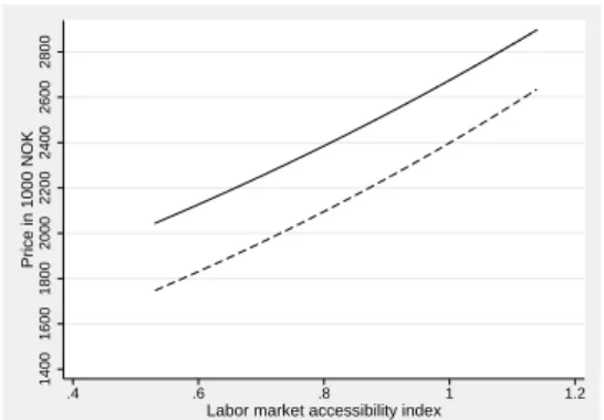
1400 1600 1800 2000 2200 2400 2600 2800 Price in 1000 NOK .4 .6 .8 1 1.2
Labor market accessibility index
b) Effects of (hypothetical) partial variations in labor market accessibility for a house located in the cbd.
Figure 3: Predicted house price gradients based on two alternative model formulations. The dashed curves are based on BM while the solid curves are based on LM8.
Similar considerations apply for the evaluation of the regional labor market accessibility effect. The two accessibility gradients in part b) of Figure 3 are based on the assumption that the standard house is located in the center of Stavanger. The dashed line in the figure is based on BM, while the solid line refers to LM8. The effect of urban attraction is also reflected in this part of Figure 3, since LM8 predicts considerably higher prices for the house located in the cbd, for any value of the labor market accessibility index. As indicated by the parameter estimates related to ACCESSIBILITY, the predicted impact on house prices of partial variations in labor
market accessibility is not sensitive to the choice between the two model alternatives.
6
Results based on semiparametric approaches
The results presented above are based on approaches where all the variables are represented through parametric specifications in the model formulation. As an alternative local peaks and valleys in housing prices can be identified in semiparametric approaches, see for instance Clapp (2003). In this section we consider model formulations where the predictor TIMECBD is the only variable that enters through a nonparametric smooth function. This represents a very flexible approach, since it imposes no a priori parametric assumptions on the smoothed function. The method is hence useful when the aim is to study potential underlying parametric structure in the data. Venables and Ripley (1997) show that smoothing splines adapt better to general smooth curves compared to for instance polynomials or lowess.
Figure 4 illustrates the results of semiparametric model formulations based on our data.
The term βlog TIMECBD in the model formulation (4) is substituted by a smoothing function
s(TIMECBD). Part a) of the figure refers to a model formulation that corresponds to the basic
model in all other respects than the specification of distance from the cbd, while the right part of the figure is based on a model formulation where labor market accessibility is not accounted for.
The plots in Figure 4 is estimated by using the mgcv (version1.3-12) package in R. This package uses a variant of generalized additive models (GAM), see for instance Hastie and Tib-shirani (1990) for a comprehensive review. In this case, penalized regression smoothing splines are estimated, by way of maximum likelihood estimation (Venables and Ripley 1997). The degree of smoothing is automatically chosen by generalized cross validation (GCV), see Wood (2000) and Wood (2001). This means that the estimated degrees of freedom for the smooth is chosen so that the GCV-score is minimized. The estimated degrees of freedom are indicated at the vertical axis of the plots in this subsection. The approach underlying Figure 4 allows a max-imum of 10 degrees of freedom. Increasing this maxmax-imum to for instance 20 leads to plots with a similar pattern, except for the most peripheral areas of the region, where the plots become more irregular. This is primarily due to the relatively small number of observations from those areas, and we have not reported results based on such more flexible non-parametric representation of
0 20 40 60 80 100 −0.4 −0.2 0.0 0.2 0.4 TIMECBD s(TIMECBD,8.66)
a) All variables in the basic model are incorporated
0 20 40 60 80 100 −0.8 −0.6 −0.4 −0.2 0.0 0.2 0.4 TIMECBD s(TIMECBD,8.47)
b) The variable representing labor market accessi-bility is ignored in the model formulation
Figure 4: Illustrations of semiparametric approaches to estimate the relationship between (loga-rithmic) housing prices and the distance from the cbd. The distance from the cbd is represented
by a smoothing functions(TIMECBD) in both model formulations.
distance from the cbd.
In Figure 4 the solid lines represent the smooth function, that is the predicted value of the dependent variable as a function of variations in TIMECBD. The dashed curves delimit approximate 95% confidence intervals of the smooth function. Following Wood (2001), the smooth is given an average value of zero in the graph. The y-axis hence shows how this predictor causes the dependent variable to alter round its mean.
The semiparametric approaches underlying the plots in Figure 4 have only marginal impact on the estimated coefficients related to the variables that still enter parametrically in the model
specification. Compared to the basic model (BM) the adjusted R2 increases somewhat in the
semi-parametric model specification where all variables in the basic model are incorporated (from 0,7396 to 0,7410), while it is somewhat lower in the model specification where labor market accessibility is not accounted for (0,7390). The increased fit resulting from the GAM model comes at the expense of the degrees of freedom. As indicated at the vertical axis in part a) of Figure 4 the degrees of freedom used for the smoothing function are 8,66. This means that the degrees of freedom used for the GAM model is 21,66, while the number of parameters
to be estimated in the basic model is 15. The GCV-score (see for instance Wood (2001)) is also slightly lower in the GAM model, but the differences are very small (BM: 0,0478, GAM: 0,0477). Notice that not even a flexible nonparametric representation of TIMECBD adds more to the explanatory power than the simple measure of traveling time from the cbd in a parametric approach.
According to the plot in part a) of Figure 4 the confidence is very narrow at locations close to the cbd, whereas the confidence bands are much wider for peripheral locations, where there are fewer observations, located further apart from each other. According to this plot a local peak seems to exist in a distance of around 32 minutes from the cbd (Bryne), while no other statistically significant irregularities are evident for the rest of the estimated path. Hence, the figure reveals no other clear hypotheses of local variables that should be included in an appropriate explanation of spatial variation in housing prices.
The gradient in the right part of Figure 4 incorporates both the urban attraction effect and the labor market accessibility effect, since labor market accessibility is not explicitly accounted for in the model formulation. In this case the irregularities to some degree are smoothed out, and the housing price gradient is predicted to be steeper than in the case where the labor market accessibility is accounted for through a separate measure. This especially applies for peripheral areas. The distance from the cbd and labor market accessibility are strongly negatively corre-lated. It is intuitively reasonable that the gradient becomes more irregular and flatter, with a wider confidence band, in part a) of the figure, where some of the effect of variations in distance is captured through the introduction of the labor market accessibility measure.
7
Concluding remarks
The main result in this paper is that the incorporation of local spatial structure characteristics only marginally improves the goodness-of fit compared to the results following from a model formulation where such local characteristics are not accounted for. In the basic model spatial structure is represented by two globally defined measures, and according to our results distance from the cbd and labor market accessibility capture most of the spatial variation in house prices. In fact, an adequate functional representation of the distance from the cbd results in satisfying values of goodness-of-fit indices, even if labor market accessibility is not explicitly accounted for
through a separate variable. This does not mean that the labor market accessibility measure only marginally contributes to explain spatial variation in house prices. As reported in Osland and Thorsen (2008) the incorporation of this variable leads to a distinction between two substantial effects in the determination of house prices: the urban attraction effect and the labor market accessibility effect. A model specification where only distance from the cbd is accounted for is biased, despite the fact that this variable satisfactorily captures the aggregate impact of the two effects.
Similarly, local spatial structure characteristics might contribute to explain spatial variation in house prices, despite the fact that they do not improve the goodness-of-fit to an appreciable extent. According to our results the specification of subcenters outside the central parts of the region contributes significantly to explain spatial variation in house prices. We found similar attraction effects that was identified for the Stavanger cbd. Our results support a hypothesis that it is in particular important to account for subcenters that are located in a long distance from the central parts of the region. This corresponds to the hypothesis that the impact of variations in distance from the subcenter is positively related to the distance from the cbd. We also find that spatial variation in house prices is significantly influenced by a variable representing the administrative centers in the most centrally located municipalities of the region, and our results indicate that house prices are positively related to the size of the intrazonal population.
We have also proposed to account for the position of a zone through a measure of relative labor market accessibility. This measure is based on comparing the values of the labor market accessibility measure of a zone to the corresponding values in neighboring zones (with a common
border). Our results on this measure give no support for the hypothesis that a high local
labor market accessibility contributes positively to house prices. One possible explanation is that negative externalities of job concentrations pull in the opposite direction. The results are somewhat more encouraging in the case where the geography is subdivided into an urban, a semi-urban, and a rural area. We find this kind of local labor market accessibility measures to be appealing, and leave further experiments on other data sets for future research, for instance for a more disaggregate subdivision of the geography into zones.
Even if the local variables introduced do not contribute considerably to an overall explanation of systematic spatial variation in house prices, they are potentially important if the ambition is
to predict prices at specific locations, like for instance, Egersund. We also find that a simple, one-parameter, functional representation of traveling time is adequate if relevant characteristics of spatial structure are explicitly accounted for. In such a case we find no significant contribution from a flexible function, represented by the quadratic term in the basic model, to capture irregularities in the house price gradient. The increased flexibility seems to be primarily required if information of relevant spatial structure characteristics is not available.
As an alternative attempt to find possible systematic spatial variation in the house price gradient originating from the cbd, we have also experimented with semiparametric approaches, where distance from the cbd is the only variable that enters through a nonparametric speci-fication. Except from an identification of relevant subcenters our experiments do not suggest alternative local measures of spatial structure. We also find that the semiparametric approaches do not outperform the parametric alternatives.
By studying the residuals we have identified a few zones where our models lead to considerable over/under predictions in house prices. One possible approach to improve goodness-of-fit is to introduce dummy-variables for such zones. We have refrained from such approaches, however, since our main ambition has been to identify how general, rather than location-specific, spatial structure characteristics affect house prices.
Despite some positive empirical findings in experimenting with local spatial structure char-acteristics, our results lead to the conclusion that distance from the cbd, in combination with a regionally defined labor market accessibility measure, explain the major part of systematic spatial variations in house prices. Our experiments also demonstrate that estimates of the ur-ban attraction effect and the labor market regional accessibility effect are insensitive to the incorporation of variables representing local spatial structure characteristics.
Appendix
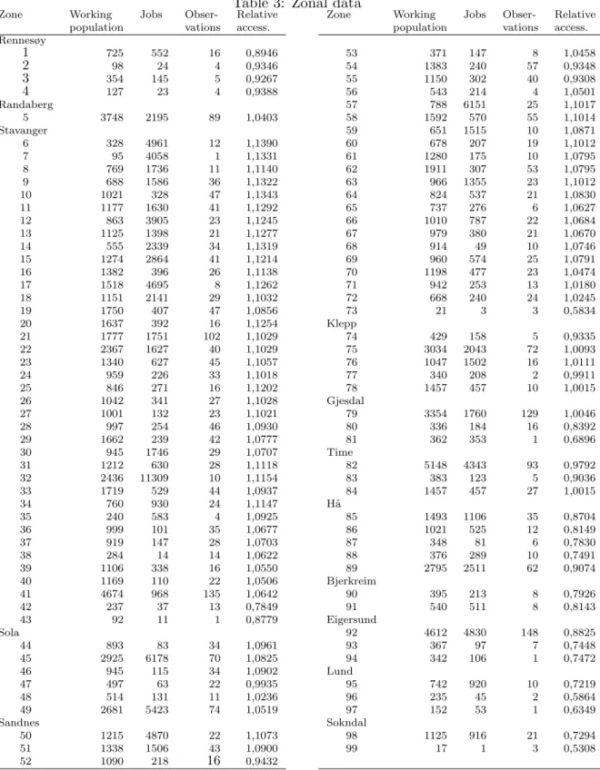
Table 3: Zonal data
Zone Working Jobs Obser- Relative Zone Working Jobs Obser- Relative population vations access. population vations access. Rennesøy 1 725 552 16 0,8946 53 371 147 8 1,0458 2 98 24 4 0,9346 54 1383 240 57 0,9348 3 354 145 5 0,9267 55 1150 302 40 0,9308 4 127 23 4 0,9388 56 543 214 4 1,0501 Randaberg 57 788 6151 25 1,1017 5 3748 2195 89 1,0403 58 1592 570 55 1,1014 Stavanger 59 651 1515 10 1,0871 6 328 4961 12 1,1390 60 678 207 19 1,1012 7 95 4058 1 1,1331 61 1280 175 10 1,0795 8 769 1736 11 1,1140 62 1911 307 53 1,0795 9 688 1586 36 1,1322 63 966 1355 23 1,1012 10 1021 328 47 1,1343 64 824 537 21 1,0830 11 1177 1630 41 1,1292 65 737 276 6 1,0627 12 863 3905 23 1,1245 66 1010 787 22 1,0684 13 1125 1398 21 1,1277 67 979 380 21 1,0670 14 555 2339 34 1,1319 68 914 49 10 1,0746 15 1274 2864 41 1,1214 69 960 574 25 1,0791 16 1382 396 26 1,1138 70 1198 477 23 1,0474 17 1518 4695 8 1,1262 71 942 253 13 1,0180 18 1151 2141 29 1,1032 72 668 240 24 1,0245 19 1750 407 47 1,0856 73 21 3 3 0,5834 20 1637 392 16 1,1254 Klepp 21 1777 1751 102 1,1029 74 429 158 5 0,9335 22 2367 1627 40 1,1029 75 3034 2043 72 1,0093 23 1340 627 45 1,1057 76 1047 1502 16 1,0111 24 959 226 33 1,1018 77 340 208 2 0,9911 25 846 271 16 1,1202 78 1457 457 10 1,0015 26 1042 341 27 1,1028 Gjesdal 27 1001 132 23 1,1021 79 3354 1760 129 1,0046 28 997 254 46 1,0930 80 336 184 16 0,8392 29 1662 239 42 1,0777 81 362 353 1 0,6896 30 945 1746 29 1,0707 Time 31 1212 630 28 1,1118 82 5148 4343 93 0,9792 32 2436 11309 10 1,1154 83 383 123 5 0,9036 33 1719 529 44 1,0937 84 1457 457 27 1,0015 34 760 930 24 1,1147 H˚a 35 240 583 4 1,0925 85 1493 1106 35 0,8704 36 999 101 35 1,0677 86 1021 525 12 0,8149 37 919 147 28 1,0703 87 348 81 6 0,7830 38 284 14 14 1,0622 88 376 289 10 0,7491 39 1106 338 16 1,0550 89 2795 2511 62 0,9074 40 1169 110 22 1,0506 Bjerkreim 41 4674 968 135 1,0642 90 395 213 8 0,7926 42 237 37 13 0,7849 91 540 511 8 0,8143 43 92 11 1 0,8779 Eigersund Sola 92 4612 4830 148 0,8825 44 893 83 34 1,0961 93 367 97 7 0,7448 45 2925 6178 70 1,0825 94 342 106 1 0,7472 46 945 115 34 1,0902 Lund 47 497 63 22 0,9935 95 742 920 10 0,7219 48 514 131 11 1,0236 96 235 45 2 0,5864 49 2681 5423 74 1,0519 97 152 53 1 0,6349 Sandnes Sokndal 50 1215 4870 22 1,1073 98 1125 916 21 0,7294 51 1338 1506 43 1,0900 99 17 1 3 0,5308 52 1090 218 16 0,9432
Note: The relative accessibility is found by dividingSj(see Equation 3) by the mean value of this measure for
References
[1] Adair A, S McGreal, A Smyth, J Cooper, and T Ryley, 2000, “House prices and accessibility:
the testing of Relationships within the Belfast urban area”,Housing studies,15699-716.
[2] Anas, A, R J Arnott, K A Small, 1998, “Urban spatial structure”, Journal of Economic
Literature,36, 3, 1426-1464.
[3] Anselin L, 1988, Spatial econometrics: methods and models. Kluwer Academic Publishers,
London.
[4] Clapp, J M, 2003, ”A semiparametric Method for Valuing Residential Locations:
Appli-cation to Automated Valuation”, Journal of Real Estate Finance and Economics, 27:3,
303-320.
[5] Dubin, R A and C H Sung, 1987, ”Spatial variation in the price of housing rent gradients
in non-monocentric cities”,Urban Studies 24, 193-204.
[6] Florax RJGM and T De Graaf (2004): ”The performance of diagnostic tests for spatial dependence in linear regression models: a meta-analysis of simulation studies”. Ch. 2 in
Advances in Spatial Econometrics. Methodology, Tools and Applications, Anselin, L, RJGM Florax and SJ Rey (eds.), Springer.
[7] Guiliano, G, and K A Small, 1991, ”Subcenters in the Los Angeles region”,Regional Science
and Urban Economics,21, 163-182.
[8] Handy, S L, 1993, ”Regional versus local accessibility: implications for nonwork travel”,
Transportation Reasearch Record, 1400, 58-66.
[9] Handy, S L, and D A Niemeier, 1997, ”Measuring accessibility: an exploration of issues and
alternatives”,Environment and Planning A,29, 1175-1194.
[10] Hansen W G, 1959, “How accessibility shapes land use”,Journal of the American Institute
of Planners 2573-76.
[11] Hastie, T and R J Tibshirani, 1990, Generalized Additive Models, London: Chapman and
[12] Heikkila E, P Gordon, J I Kim, R B Peiser, H W Richardson, 1989, “What happened to
the CBD-distance gradient?: land values in a polycentric city”,Environment and Planning
A21 221-232.
[13] Jones, C, 1988, ”The definition of housing market areas and strategic planning, Urban
Studies,39, 3, 549-564.
[14] Kennedy P, 2003, A Guide to Econometrics, The MIT Press.
[15] Li M M and H J Brown, 1980, “Micro-neighbourhood externalities and hedonic prices”,
Land Economics 56125-140.
[16] McDonald, J F, 1987, ”The identification of urban employment subcenters”, Journal of
Urban Economics,21, 242-258.
[17] McMillen, D P, 2001, ”Nonparametric employment subcenter identification”, Journal of
Urban Economics, 50. 448-473.
[18] McMillen, D P, 2003, ”Neighborhood house price indexes in Chicago: A Fourier repeat
sales approach”,Journal of Economic Geography, 3, 57-73.
[19] McMillen, D P, 2004, ”Employment subcenters and home price appreciation rates in
metropolitan Chicago”, in: J P LeSage and K Pace, eds., Advances in Econometrics,
Vol-ume 18: Spatial and Spatiotemporal Econometrics, Elsevier, New York, 237-257.
[20] Osland, L, I Thorsen, and J P Gitlesen, 2005, ”Housing price gradients in a geography with one dominating center”, Working papers in economics, Department of Economics, University of Bergen, no. 06/05.
[21] Osland, L, I Thorsen, and J P Gitlesen, 2007, ”Housing price gradients in a geography with
one dominating center”,Journal of Real Estate Research, vol. 29, no. 2, 321-346.
[22] Osland, L and I Thorsen, 2008, ”Effects of housing prices of urban attraction and labor market accessibility”, to appear in Environment and Planning A.
[23] Richardson, H W, P Gordon, M Jun, E Heikkila, R Peiser, and D Dale-Johnson, 1990,
”Residential property values, the CBD, and multiple nodes: Further analysis”,Environment
[24] Venables, W N and B D Ripley, 1997, Modern Applied Statistics with S-Plus, Springer [25] Waddell, P, B J L Berry, and I Hoch, 1993, ”Residential property values in a multinodal
urban area: new evidence on the implicit price of location,Journal of Real Estate Finance
and Economics,22829-833
[26] Wood, S N, 2000, ”Modelling and smoothing parameter estimation with multiple quadratic
penalties”,Journal of the Royal Statistical Society B, 62, 413-428.
[27] Wood, S N, 2001,mgcv: GAMs and Generalized Ridge Regression for R, R News.
[28] Yinger, J, 1979, ”Estimating the relationship between location and the price of housing”,
Department of Economics University of Bergen Fosswinckels gate 6 N-5007 Bergen, Norway Phone: +47 55 58 92 00 Telefax: +47 55 58 92 10 http://www.svf.uib.no/econ