DOI 10.1007/s11146-009-9231-x
Fractional Cointegration Analysis of Securitized
Real Estate
Camilo Serrano·Martin Hoesli
Published online: 7 January 2010
© Springer Science+Business Media, LLC 2009
Abstract This paper uses fractional cointegration analysis to examine whether
long-run relations exist between securitized real estate returns and three sets of variables frequently used in the literature as the factors driving securi-tized real estate returns. That is, we examine whether such relationships are characterized by long memory (long-range dependence), short memory (short-range dependence), mean reversion (no long-run effects) or no mean reversion (no long-run equilibrium). The forecasting implications are also considered. Empirical analyses are conducted using data for the U.S., the U.K., and Australia. We find strong evidence of fractional cointegration between securitized real estate and the three sets of variables. Such relationships are mainly characterized by short memory although long memory is sometimes present. The use of fractional cointegration for forecasting purposes proves particularly useful since the start of the financial crisis.
C. Serrano
University of Geneva (HEC and GFRI), 40 boulevard du Pont-d’Arve, 1211 Geneva 4, Switzerland
e-mail: camilo.serrano@unige.ch M. Hoesli (
B
)University of Geneva (HEC, GFRI and SFI), 40 boulevard du Pont-d’Arve, 1211 Geneva 4, Switzerland
e-mail: martin.hoesli@unige.ch M. Hoesli
University of Aberdeen (Business School), Edward Wright Building, Aberdeen AB24 3QY, Aberdeen, Scotland, UK
M. Hoesli
Keywords Fractional cointegration·Fractionally Integrated Error Correction Model (FIECM)·Forecasting·Multifactor models· Securitized real estate·REITs
JEL Classification G17·G11·C53
Introduction
Although real estate security markets have been bearish recently, they have overall grown substantially in the last decade both in the U.S. and internation-ally. An increasing number of portfolio managers are considering such vehicles as a substitute or in addition to direct real estate holdings. Three models have primarily been used in the literature when examining the explanatory factors and the predictability of securitized real estate returns. One model has considered the linkages with bond and inflation related variables (Chan et al.1990), the second model the linkages with bond and performance related variables (Liu and Mei1992), while the third has focused on the relationships with financial assets (i.e., stocks and bonds) and real estate (Clayton and MacKinnon2003). Defining and describing the linkages between those sets of variables and securitized real estate, is thus of importance as this could provide essential insight for forecasting purposes. A question that arises is whether securitized real estate is fractionally cointegrated with the variables used in these models, and if so, to which degree, as this would allow the characterization of their long-run equilibrium relationships.
This question is of outmost importance as most of the research studying the explanatory factors and the predictability of securitized real estate returns uses variations of these three models. This paper provides a contribution to the existing literature by establishing the nature of the nonlinear linkages between securitized real estate and each of the three sets of variables. That is, by estimating the degree of cointegration with each set of variables, we determine whether the relationships exhibit long memory (long-range dependence), short memory (short-range dependence), no long-run effects (mean reversion) or no long-run equilibrium (no mean reversion; the process drifts away from its equilibrium permanently).1 Therefore, the paper’s main contributions are to identify the dynamics that govern the relationships between securitized real estate and the three sets of variables, and to determine whether these models may be successfully used to forecast securitized real estate returns and construct profitable trading strategies.
Data for the U.S., the U.K., and Australia are used. These countries are three of the six largest securitized real estate markets and account for 41% of the global securitized real estate market capitalization as of 2009Q2. Due
1Long (short) memory entails that the correlation with past quarterly observations decays slowly (exponentially).
to data availability, the analysis for the U.S. is for 1980–2009Q2, whereas the time period is 1987–2009Q2 for the U.K. and Australia. The major difference between these markets is that in the U.S. and Australia, real estate securities have tax-transparency (REIT status) during the whole period studied, while in the U.K., REIT status was only established at the end of the time period considered (in 2007). Additionally, REITs comprise development and building activities. Another important difference concerns the leverage employed by these companies in the different countries, with real estate securities in the U.S. being far more leveraged than real estate securities in the U.K. and in Australia.2
Our findings suggest that securitized real estate returns are fractionally cointegrated with the three sets of variables (i.e., the variables used by Chan et al.1990; Liu and Mei1992; and Clayton and MacKinnon2003). The degree of fractional cointegration varies somewhat across models and across coun-tries. However, all of the relationships are characterized by short memory and in a few instances there is long memory. The use of fractional cointegration for forecasting purposes proves especially useful since the start of the financial crisis (i.e., since 2007). Overall, the use of the three models in active investment strategies generate economically significant excess returns over a passive buy-and-hold investment. The best results are obtained with the financial and real estate factors model.
The paper is organized as follows. The next section offers a review of the relevant literature. The third section provides a description of the data, while the fourth section presents the methodology. The penultimate section contains the results, and the last section provides some concluding remarks.
Literature Review
Economic variables have been commonly used in the financial economics literature to examine the behavior and predictability of asset returns. Chen et al. (1986) test whether innovations in macroeconomic variables affect stock market returns. Keim and Stambaugh (1986) try to identify ex ante observable variables that reliably predict ex post risk premiums on a wide range of assets. Campbell (1987) presents evidence that the state of the term structure of interest rates predicts excess returns of stocks, bills, and bonds. Fama and French (1989) present empirical evidence that the excess returns of stocks and bonds may be forecasted. More recently, Laopodis (2006) examines the dynamic interactions among the stock market, economic activity, inflation, and monetary policy, and finds that the relationships vary across time. All of these studies pertain to the U.S. stock market.
2As of the end of 2008, the average debt/equity ratio of the five largest real estate securities in each country was 3.19 in the U.S., 1.68 in the U.K., and 0.95 in Australia.
For the U.K., Diacogiannis (1986), Poon and Taylor (1991), and Cheng (1995) show that the macroeconomic variables of Chen et al. (1986) are not useful to predict stock returns. However, various economic variables are analyzed in the U.K. by Beenstock and Chan (1986), Clare and Thomas (1994), Priestley (1996), and Antoniou et al. (1998), and some of the variables appear to be priced in the stock market. In Australia, Groenewold and Fraser (1997) and Yao et al. (2005) find that the factors priced in the stock market overlap considerably with those found in the U.S. At an international level, more recent studies examining the effects of economic variables on global stock market returns include Cheung and Lai (1999), Cheung and Ng (1998), Aylward and Glen (2000), Fifield et al. (2002), and Wongbangpo and Sharma (2002). Although the results lack consistency across studies, there is some evidence that interest rate, inflation, and economic activity variables, as well as bond related variables have explanatory and predictive power.
In the securitized real estate literature for the U.S., many studies have also examined the explanatory (Chan et al.1990; McCue and Kling1994; Ling and Naranjo1997; Chen et al.1998; Payne2003; Ewing and Payne2005) and pre-dictive (Liu and Mei1992; Mei and Liu1994; Bharati and Gupta1992) power of several economic variables. In the U.K., it has been addressed by Brooks and Tsolacos (1999) and Brooks and Tsolacos (2001), and at an international level Brooks and Tsolacos (2003) analyze five European countries and Liow and Webb (2009) investigate four of the largest global securitized real estate markets. As in the financial economics literature, it appears that the number, as well as the factors that have an impact, vary across time and across countries. The two most representative papers are those of Chan et al. (1990) and Liu and Mei (1992). Chan et al. (1990) use the macroeconomic variables proposed by Chen et al. (1986) and find that the spread between high- and low-grade bonds, the slope of the term structure of interest rates, and unex-pected inflation have explanatory power, while changes in exunex-pected inflation and industrial production do not. Liu and Mei (1992), on the other hand, examine bond and performance related variables and find that cap rates are an important determinant of EREITs expected excess returns as they contain useful information about the general risk conditions in the economy.
A third alternative contemplated in the literature to explain and forecast securitized real estate returns is to rely on the hybrid nature of this asset class. Securitized real estate is viewed as a hybrid asset of stocks, bonds, and real estate (Clayton and MacKinnon2001,2003). The reason for this is that real estate securities are stocks with generally stable cash flows derived from income-producing real estate. Thus, stock-like characteristics appear in real estate securities as they are publicly traded, bond-like features emerge from the generally long-term fixed leases that generate a fixed income, and real estate-like attributes arise from the underlying real estate assets.
Abundant literature exists linking securitized real estate to financial assets (Peterson and Hsieh1997; Karolyi and Sanders1998; Ling and Naranjo1999), as well as to real estate (Giliberto1990; Gyourko and Keim1992; Mei and Lee 1994; Barkham and Geltner 1995). Overall, the general conclusions at
an international level suggest that securitized real estate returns are positively related to stock and real estate returns, but negatively related to bond returns (Hoesli and Serrano2007). The only study that examines the usefulness of such factors to forecast securitized real estate returns is that of Serrano and Hoesli (2007). They use the hybrid nature of EREITs to compare the predictive potential of four different model specifications with time varying coefficient (TVC) regressions, VAR systems, and neural networks models. Their results show that the best predictions are obtained with the neural networks model, particularly when stock, bond, real estate, size, and book-to-market factors are used.
Some research has also examined whether real estate securities are cointe-grated with other assets or economic variables. Wilson and Okunev (1999) find no evidence to suggest long co-memories between stock and securitized real estate markets in the U.S. and the U.K., but some evidence of this in Australia. Glascock et al. (2000) report that U.S. REITs were cointegrated with bonds and inflation until 1992 and to stocks, particularly small caps, thereafter. A generalized version of cointegration, named fractional cointegration, has been used to analyze the existence of nonlinear long-run relationships. In the finance literature, it was initially employed by Cheung and Lai (1993) in an examination of purchasing power parity, and by Baillie and Bollerslev (1994) in an exchange rate context. In the securitized real estate literature, Liow and Yang (2005) examine several economies of the Asia-Pacific region and test for fractional cointegration between securitized real estate prices, stock prices, and key macroeconomic factors (GDP, inflation, money supply, short-term interest rate, and exchange rate). Some support for fractional cointegration is reported; however, the results lack robustness as most of their estimations are not statistically significant.
Overall, the existing literature examining the explanatory factors and the predictability of securitized real estate returns has focused on testing variations of the models proposed by Chan et al. (1990), Liu and Mei (1992), and Clayton and MacKinnon (2003). No study to date has examined if nonlinear long-run relations exist between securitized real estate and these commonly used models. This paper contributes to the literature by identifying their degree of fractional cointegration, i.e., by depicting the nature of the long-run nonlinear relationships between securitized real estate and the three most commonly used models in the literature to explain and forecast its returns. A second contribution is that we analyze the forecasting implications of using such findings in active investment strategies.
Data
The data used in this study were mainly sourced from Thomson Datastream and cover the period 1980-2009Q2 for the U.S., and 1987–2009Q2 for Australia and the U.K. Based on the GPR General Global data as of 2009Q2, these three countries are, respectively, the first, fifth, and sixth largest securitized real
estate markets in the world in terms of market capitalization. Together, they account for 41% of global securitized real estate markets (the U.S.=25.7%, Australia=8.3%, and the U.K.=6.7%). The starting dates of the samples were dictated by the availability of the corporate bonds data in the U.S., the direct real estate data in the U.K., and the government bonds data in Australia, respectively, while the frequency used was dictated by several of the variables whose data are released on a quarterly basis only. Data are in local currency. For securitized real estate, the FTSE/NAREIT All REITs total return index is used for the U.S. and the GPR General Property Share total return index for the U.K. and Australia.3Returns are forecasted by means of three models. Two models use economic variables and a third one uses financial and real estate factors.
A summary of the forecasting variables used in this paper is provided in Table 1. Panel A contains the raw economic series. The CPI is calculated by the Bureau of Labor Statistics in the U.S., and by the Organization for Economic Co-operation and Development (OECD) in the U.K. and Australia. The Treasury-bill is obtained from the Financial Times in the U.S., the Office for National Statistics in the U.K., and Datex in Australia. Concerning the corporate bonds data, it is from Citigroup. The two sets of economic variables are shown in Panel B: First, the set used by Chan et al. (1990), then the one used by Liu and Mei (1992). The former set includes bond and inflation related variables, while the latter comprises bond and performance related variables. Finally, the financial and real estate factors employed by Clayton and MacKinnon (2003) appear in Panel C. Such factors include Datastream’s total return stock index, St, Datastream’s 10-year total return government
bond index, Bt, and for the real estate factor, REt, the NCREIF Property
Index (NPI) in the U.S., the IPD index in the U.K., and the Mercer Unlisted Property Fund Index (MUPFI) in Australia.4For the U.S., we also use MIT’s transaction-based index (TBI) for the slightly shorter time period for which it is available, (1984–2009Q2).5
Appraisal-based real estate returns indices are used to allow for compar-ison of the results across countries as there are no transaction-based indices available in the U.K. and Australia. One common problem with appraisal-based real estate returns, however, is the smoothing issue (Geltner 1993; Fisher et al.1994). Therefore, we desmooth the real estate indices using the
3The FTSE/NAREIT series starts in 1977Q4 for the U.S. and in 1989Q4 for the U.K. and Australia, while the GPR series are available for the three countries since 1983Q4. Hence, different data sources are used for securitized real estate in order to have the longest series possible in each country.
4We use the MUPFI, a widely used benchmark for the Australian direct real estate market, as the Property Council of Australia (PCA) index is only available at a quarterly frequency since 1995Q2 (at a semi-annual frequency since 1984H2). At a semi-annual frequency, the correlation between the PCA index and the MUPFI is 0.96 for the period 1985H1 to 2009H1.
Table 1 Sets of variables examined
Symbol Variable Data source or measurement Panel A: Raw economic series and sources
It Inflation Consumer price index
TBt Treasury-bill rate 3-month Treasury-bill rate in the U.S. and the U.K.,
and 3-month Interbank middle rate in Australia Bt Long-term Datastream’s 10-year total return government bond
government bonds index
AAAt Corporate AAA bonds Citigroup’s corporate AAA/AA bond index
BBBt Corporate BBB bonds Citigroup’s corporate BBB bond index
Panel B: Economic variables Chan et al. (1990)
TSt Change in term structure Bt-TBt RPt Change in risk premium BBBt-AAAt
EIt Expected inflation Fama and Gibbons (1984) EIt Change in expected EIt+1-EIt
inflation
UIt Unexpected inflation It-EIt
Liu and Mei (1992)
TBt Treasury-bill rate 3-month Treasury-bill rate in the U.S. and the U.K.,
and 3-month Interbank middle rate in Australia YSt Yield spread AAAt-TBt
DYt Stocks dividend yield Datastream’s stock’s dividend yield index
CRt REITs Cap. Rate FTSE/NAREIT All REITs dividend yield index in the
U.S. and GPR General dividend yield index in the U.K. and Australia
Panel C: Financial and real estate factors
St Stock factor Datastream’s total return stock index
Bt Bond factor Datastream’s 10-year total return government bond
index
REt Real estate factor NCREIF Property Index (NPI) and MIT’s Transaction
Based Index (TBI) in the U.S., IPD index in the U.K., and Mercer’s Unlisted Property Fund Index (MUPFI) in Australia
For Australia, the Treasury-bill rate is not available for the whole period, so the Interbank 3-month middle rate is used. The correlation over the shorter common time period for which both interest rate variables are available (1986Q2–2002Q2) is 0.97
Investment grade bonds data are not available in the U.K. and Australia for the whole period, so these variables are proxied using U.S. data. The correlation between U.S. and U.K. AAA bonds is 0.75, while the correlation is 0.62 for BBB bonds for the period 1997Q1–2009Q2. In Australia, these correlations are 0.79 and 0.48, respectively, for the period 2000Q4–2009Q2
As done by Chan et al. (1990), expected inflation is calculated using Fama and Gibbons (1984), i.e.,
EIt=TBt−1−121 st−=12t−1[TBs−1−Is]
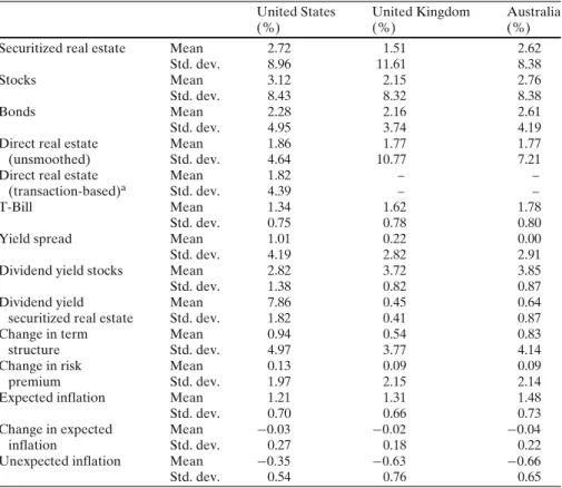
Fisher et al. (1994) approach. Their methodology is conceived to desmooth quarterly indices by adding to the first-order AR term that captures appraiser’s behavior, a fourth-order AR term to take into account the strong seasonality that characterizes such indices. Summary statistics of all the variables used are available in Table2.
Table 2 Summary statistics, 1980–2009Q2 for the U.S. and 1987–2009Q2 for the U.K. and Australia (quarterly data)
United States United Kingdom Australia
(%) (%) (%)
Securitized real estate Mean 2.72 1.51 2.62
Std. dev. 8.96 11.61 8.38
Stocks Mean 3.12 2.15 2.76
Std. dev. 8.43 8.32 8.38
Bonds Mean 2.28 2.16 2.61
Std. dev. 4.95 3.74 4.19
Direct real estate Mean 1.86 1.77 1.77
(unsmoothed) Std. dev. 4.64 10.77 7.21
Direct real estate Mean 1.82 – –
(transaction-based)a Std. dev. 4.39 – –
T-Bill Mean 1.34 1.62 1.78
Std. dev. 0.75 0.78 0.80
Yield spread Mean 1.01 0.22 0.00
Std. dev. 4.19 2.82 2.91
Dividend yield stocks Mean 2.82 3.72 3.85
Std. dev. 1.38 0.82 0.87
Dividend yield Mean 7.86 0.45 0.64
securitized real estate Std. dev. 1.82 0.41 0.87
Change in term Mean 0.94 0.54 0.83
structure Std. dev. 4.97 3.77 4.14
Change in risk Mean 0.13 0.09 0.09
premium Std. dev. 1.97 2.15 2.14
Expected inflation Mean 1.21 1.31 1.48
Std. dev. 0.70 0.66 0.73
Change in expected Mean −0.03 −0.02 −0.04
inflation Std. dev. 0.27 0.18 0.22
Unexpected inflation Mean −0.35 −0.63 −0.66
Std. dev. 0.54 0.76 0.65
aThe summary statistics for the transaction-based data are for the period 1984–2009Q2
Methodology
The debate concerning the variables to include in a forecasting model of asset returns is probably endless. An optimal model that remains robust through different time periods, countries, and asset classes, is hardly conceivable. For securitized real estate, variations of three sets of variables have been mainly used in the literature when examining the explanatory factors and the predictability of this asset class. These sets of variables derive from the models used by Chan et al. (1990), Liu and Mei (1992), and Clayton and MacKinnon (2003). Therefore, an examination of the long-run linear or nonlinear relation-ships depicted by these models is warranted to understand better the impacts of these factors and their usefulness for forecasting purposes. Depicting such past relationships is not a guarantee for future forecasting performance, but precious insights should be gained. Fractional cointegration analysis offers the appropriate framework to analyze the explanatory power of these models, as well as their forecasting potential.
Fractional Cointegration
First, we characterize the long-run dynamics that could link securitized real estate to the three models tested. For that purpose, fractional cointegration tests are performed. That is, we estimate the degree of cointegration, I(d), between the dependent variable and the three specifications used. We use this generalized version of cointegration to avoid making a linearity assumption in the relationship. Such estimation allows to identify the presence or lack of cointegration, and ultimately, the degree of cointegration which enables the characterization of the relationship between securitized real estate and each set of explanatory variables. Depicting these long-run linkages is important to understand how these variables interacted with securitized real estate returns in the past, as this may prove useful to infer future interactions.
Empirical studies in macroeconomics and finance usually involve the use of non-stationary series such as price levels, exchange rates, income, consumption or money demand. Rendering such series stationary by differencing, taking logs, or making any other transformation has been a common practice in order to analyze the resulting series with Box and Jenkins methods or with VARs. However, an interesting body of literature concerns the analysis of non-stationary time series. As such, the level series of securitized real estate and of the variables are used in the three specifications to determine if they are fractionally cointegrated, i.e., to establish whether linear or nonlinear long-run equilibrium relationships exist among the variables.
A time series is said to be integrated of order d, denoted I(d), if it can achieve stationarity after differencing it d times; d being an integer. Engle and Granger (1987) demonstrate that a linear combination of two or more non-stationary series may be non-stationary. Such series are said to be cointegrated. The stationary linear combination is called the cointegrating equation and may be interpreted as a long-run equilibrium relationship among the variables. The standard approach used to test for cointegration is the linear Full Information Maximum Likelihood (FIML) technique of Johansen (1988,1991).6
Fractional cointegration examines a broader characterization of a long-run economic relation than cointegration. It refers to the case in which two processes with the same degree of integration have an equilibrium error that is
I(d), with d defined as any real number less than one. This relaxes the I(0)
error term requirement in the traditional cointegration specification. Thus, fractional cointegration associates the existence of a long-run relationship with mean reversion in the error term, rather than requiring both mean reversion and stationarity.
The presence of a long-run equilibrium relationship when d is a non-integer real number less than one entails that nonlinearities are at play and that the
equilibrium error may still be mean-reverting. The mean reversion behavior depends primarily on the value of the fractional differencing parameter, d. The interpretation of the degree of integration is as follows (Hosking1981). A process displays long memory (long-range dependence) when0<d<0.5, short memory (short-range dependence) when −0.5<d<0, no long-run effect (mean reversion) when0.5<d<1, and no mean reversion (the process drifts away from its equilibrium permanently) when d>1. Long- and short-range dependent processes are characterized by their autocovariance func-tions. In short-range dependent processes, the coupling between values at different points in time decreases rapidly as the time difference increases. That is not the case in long-range dependent processes, where the coupling lasts much longer. Therefore, the autocovariance function exhibits an exponential decay near zero in the presence of short memory and a hyperbolic decay when there is long memory. Stated differently, a long or short memory process may be defined according to whether its correlations have an infinite or finite sum. To estimate the fractional cointegration parameter, d, the following four-step procedure is followed. First, we estimate the order of integration for each series as it must be the same for all the series in order to perform cointegra-tion analysis. For that purpose, Augmented Dickey-Fuller (ADF) tests are performed to determine the presence of a unit root (non-stationarity) in all the series. Then, a cointegration regression is performed for each specification tested:
Model of Chan et al. (1990)
Yt=α0+α1T St+α2RPt+α3EIt+α4EIt+α5U It+zat (1)
Model of Liu and Mei (1992)
Yt=θ0+θ1T Bt+θ2Y St+θ3DYt+θ4C Rt+zb t (2)
Financial and real estate factors model
Yt=ψ0+ψ1St+ψ2Bt+ψ3REt+zct (3)
where Yt is the level of the securitized real estate series, the explanatory
variables are those defined in Table1, and z·tare the respective residual series.
Given that we use a quarterly frequency, the small number of observations available to calculate the degree of cointegration results in estimations with large confidence intervals, that are therefore not significant. To increase the robustness of the estimation of the degree of cointegration, we use a boot-strap procedure on the residual series, z·t. The bootstrap procedure consists
in drawing 100 random samples with replacement of the same size as the original sample. The bootstrapped residual series, are then examined for the existence of fractional cointegration by estimating the fractional cointegration
parameter, d, with Geweke and Porter-Hudak’s (1983) fractional differencing test for long memory. Basically, this technique examines the behavior of the spectral density near zero. This means that the log periodogram is regressed on log frequencies around zero to calculate the slope coefficient. This coefficient provides a consistent estimator of the fractional differencing parameter. The spectral regression is as follows:
ln(Iu(ωj))=α+βln
4 sin2(ωj/2)
+εt f or j=1,2, . . . ,n (4)
where Iu(ωj)= 2π1T |Tt=1eitω(zt−z)|2 is the periodogram of ztat frequency
ωj, β=1−d, εt=ln(Iu(ωj)/fu(ωj)) is assumed to be i.i.d. with theoretical
asymptotical mean and variance equal to 0 andπ2/6, respectively, T is the
number of observations, and n= f(T)=Tμ for 0< μ <1is the number of low-frequency ordinates used in the regression. Geweke and Porter-Hudak (1983) suggest to useμ=0.55, 0.575, and 0.60 to show the sensitivity of the test to the length of the spectral regression.7For the sample size function n=Tμ, we report results forμ=0.575 as the differences with the other two values is insignificant due to our bootstrapping procedure.
Since the mean reversion behavior of the equilibrium error depends more on the range than on the exact value of the fractional differencing parameter,
d, we provide the confidence intervals at a 95% level. The confidence intervals
give a clearer idea of the deviations from the main behavior of the residual series of the cointegration regression and, therefore, of the linkages between the dependent variable and the three models. The critical values for the GPH test are nonstandard, so those derived from the standard distribution cannot be used. In fact, the residual series of the cointegration regression tends to be biased toward being stationary. Therefore, we employ the critical values provided by Sephton (2002) who performs Monte Carlo estimates of the critical values to use in fractional cointegration tests.
Fractionally Integrated Error Correction Model
The presence of a cointegrating relation forms the basis of the Error Cor-rection Model (ECM). Even though cointegrated variables display a long-run equilibrium relationship, short-long-run dynamics cause deviations from this equilibrium. This short-run behavior may be tied to the long-run equilibrium by the error correction term. The advantage of modeling the cointegration relationship by a fractional process lies in its incorporation of the effects of
7Note that a large value of n may contaminate the estimation of d due to the high/medium frequency components, but a small value of n will lead to imprecise estimates due to the limited degrees of freedom.
long and short memory. While the ECM only takes into account the first-order lag of the cointegration residual series, the Fractionally Integrated Error Correction Model (FIECM) incorporates a long history of past cointegration residuals. The FIECM may be defined as follows:
lnYt=φ0+ I i=1 φilnXt−i+δ (1−L)d−(1−L)zt−i+εt (5)
wherelnYt is the logarithmic difference of the level securitized real estate
series,lnXt−i is the logarithmic difference of the lagged set of explanatory
variables in their levels,8andδ[(1−L)d−(1−L)]z
t−iis the fractionally
inte-grated error correction term in which L is the lag operator, d is the order of integration, and ztis the vector of residuals from the cointegration regression.
The polynomial within the square brackets can be expanded so that the coefficient of zt−iis equivalent toδ(i−d)/{(−d)(i+1)}, where(·)is the
gamma function defined as(x)=0∞tx−1e−tdt for x>0and as(x)= (x+1)
x
for x<0.
A FIECM for each of our three models is used to produce one-quarter-ahead forecasts of securitized real estate total returns. The forecasts are con-structed dynamically using a rolling window with 50 observations for in-sample parameter estimation. Out-of-sample forecasts are obtained by re-estimating the parameters at each step and shifting the window sample by one observation until the whole sample is exhausted. The forecasts are performed over 35 out-of-sample quarters for the three countries in order to use a common period (i.e., 2000Q4–2009Q2). Such forecasts are employed in an active trading strategy that is benchmarked against a buy-and-hold investment. Under the assumption that an investor takes a long position either on real estate securities or on the risk free asset, the following trading rules are applied. If securitized real estate return forecasts are higher than the risk free asset’s return, the investor will go long on real estate securities; otherwise the investor will go long the risk free asset. Potential gains are put into perspective with the transaction costs associated with such strategies.
Empirical Results
Fractional Cointegration Results
Augmented Dickey-Fuller (ADF) tests are performed on the level of all the series used to determine the presence of a unit root. All the series are non-stationary (i.e., they have a unit root) except for unexpected inflation,
8The optimal number of lags used for each set of explanatory variables is determined according to the Schwarz Bayesian information criterion (SBC). The longest specification tested included four lags and the SBC criterion led to an optimal number of lags of one for the three models.
U It, in the three countries. Since cointegration analysis requires the series to
be non-stationary, this variable is omitted from the cointegration regression of the Chan et al. (1990) specification. Table3shows the estimated fractional cointegration coefficients, d, with their respective confidence intervals, for each of the models in each country. Overall, we find strong evidence of fractional cointegration between securitized real estate and the three models examined. The degree of fractional cointegration, d, falls in the(−0.5<d<0)
range for all the specifications tested in all the countries. In some cases, the confidence intervals slightly overlap with the(0<d<0.5)range. Therefore, we conclude that the relation of securitized real estate with the three models is generally governed by short-range dependence (short memory), although there are also some signs of long-range dependence (long memory). Such results indicate that there should be some predictability. In fact, past quarterly observations should provide useful information about the future behavior of securitized real estate. Where short memory has been identified, the last quarters will contain helpful information, and where long memory is also present, several quarters further back will also provide some insight.
More specifically, we find that securitized real estate exhibits strictly short memory with the specification of Chan et al. (1990) in Australia, with the model of Liu and Mei (1992) in the U.S., and with the financial and real estate factors specification in the three countries. The findings for the financial and real estate factors remain unchanged regardless of the real estate index used, i.e., whether an unsmoothed appraisal-based index or a transaction-based index is employed in the model. Short memory is also the predominant relation identified between securitized real estate and the specification of Chan et al. (1990) in the U.S. and the U.K., and with the specification of Liu and Mei (1992) in the U.K. and Australia. Slight evidence of long memory is also found for the model of Chan et al. (1990) and an even stronger evidence for the model of Liu and Mei (1992).
Forecasting Results
The trading results for each of the forecasting models and countries are shown in Table4. Overall, the empirical results show evidence of predictability of securitized real estate returns when the models of Chan et al. (1990), Liu and Mei (1992), and Clayton and MacKinnon (2003) are employed for forecasting purposes. All of the models outperform the buy-and-hold strategy for the 35 out-of-sample forecasts in all the countries except for the Liu and Mei (1992) model in Australia. The best performance is obtained by the financial and real estate factors model in the three countries.9
9In the U.S., this is true when the transaction-based data are employed, but not when the unsmoothed appraisal-based data is used.
Table 3 Estimated fractional cointegration coefficients Chan et al. ( 1990 ) L iu and M ei ( 1992 ) Financial and real estate factors d 95% Confidence interval d 95% Confidence interval d 95% Confidence interval United States − 0 . 09 [ − 0 . 27 0.08] − 0 . 27 [ − 0 . 45 − 0 . 10 ] − 0 . 34 [ − 0 . 48 − 0 . 19 ] − 0 . 20 † [ − 0 . 34 − 0 . 07 ] United Kingdom − 0 . 18 [ − 0 . 38 0.02] − 0 . 06 [ − 0 . 26 0.14] − 0 . 26 [ − 0 . 43 − 0 . 09 ] Australia − 0 . 30 [ − 0 . 50 − 0 . 10 ] − 0 . 03 [ − 0 . 23 0 . 17 ] − 0 . 28 [ − 0 . 45 − 0 . 11 ] This table shows the fractional cointegration coefficients estimated with equation (4), ln ( Iu (ωj )) = α + β ln ( 4s in 2(ω j / 2 )) + εt ,o n the bootstrapped residuals from the cointegration regressions. T hree sets of variables are considered: the ones u sed b y C han e t a l. ( 1990 ), those o f L iu and M ei ( 1992 ), and the financial a nd real estate factors u sed b y C layton and M acKinnon ( 2003 ) For the sample size function n = T μ, w e report results for μ = 0 . 575 . T he table a lso reports the 95% confidence intervals †Estimation w ith the transaction-based d ata since 1984. The d egree of cointegration for the same sample period using the unsmoothed a ppraisal-based data is − 0 . 22 , w ith a confidence interval of [ − 0 . 37 − 0 . 07 ] Table 4 Trading strategy results Chan et al. ( 1990 ) L iu and M ei ( 1992 ) Financial and real estate factors B uy-and-hold Annual R ound-trip Annual R ound-trip Annual R ound-trip Annual return (%) transaction costs (bp) return (%) transaction costs (bp) return (%) transaction costs (bp) return (%) United States 12.52 1417 11.51 1626 9.46 598 4.93 12.99 † 1022 United Kingdom 3.02 535 5.64 942 7.84 808 − 0 . 16 Australia 10.88 3076 0.39 0 14.11 2185 1.95 This table shows the annual returns on the a ctive trading strategies with the three forecasting specifications, a s w ell a s the buy-and-hold strategy for the 35 out-of-sample period ending 2009Q2. Transaction costs which w ould render the active strategy equivalent to the passive one are a lso shown. This mean st h a ti f transaction costs were as high as those shown in the table, the costs generated by the a ctive trading strategy will upset the p rofits, a nd no excess retu rns o ver the buy-and-hold investment w ill be generated †Results u sing the transaction-based d ata (TBI)
These results continue to hold in the presence of transaction costs. Transac-tion costs are taken into account by calculating the amount that would render the active strategy’s profits equivalent to the buy-and-hold profits. As reported in Table 4, the costs associated with such strategies cover comfortly the average round-trip execution costs; 30 basis points as estimated by Chan and Lakonishok (1993). Therefore, the active investment strategies provide eco-nomically significant outcomes during the period studied. The results confirm that the long-run relations depicted above (i.e., the existence of short memory and to a lesser extent of long memory, between securitized real estate returns and the three sets of variables) lead to economically significant securitized real estate return predictions.
The analysis of the trading strategies through time provides helpful insights about the performance of the forecasts. Figures1,2, and3, depict the out-of-sample performance of the active trading strategies and of the buy-and-hold strategy in the U.S., the U.K., and Australia, respectively. In general, we see that during the bull period, the active strategies follow the buy-and-hold but they slightly underperform it. However, the FIECM forecasts prove to be very useful during the crisis. The outliers, common in financial crises, create short term disequilibriums from the long-run equilibrium relation in each of the three models. Those disequilibriums are captured by the FIECM term, and even though the turning point is difficult to identify, the forecasts produce the correct signals during a large part of the bear market.
Figure 1 shows that the three models avoid the steep drop of the U.S. market during 2008Q4 and 2009Q1 where the market fell by 55%. Another interesting finding is that the financial and real estate factors model using the
Fig. 2 Out-of-sample performance of the active trading strategies in the U.K., 2000Q3–2009Q2
transaction-based data outperforms the one using the unsmoothed appraisal-based data during almost all the period. This result is intuitively appealing as the information content of the TBI should more clearly reflect the direct real estate market than the NCREIF. More so, the model using the TBI anticipates the market drop completely as it signals the active trading strategy to get out
of the REIT market in 2007Q3 and thus avoids the bear market that starts the following quarter.
In the U.K. (Fig.2), the model of Liu and Mei (1992) outperforms the buy-and-hold strategy both during the bull and the bear markets. Albeit the other two models outperform the buy-and-hold strategy for the whole sample period, these strategies produce limited results as their underperformance during the bull market is significant and the bear market is only imperfectly foreseen. The poor performance of the Chan et al. (1990) model is in line with the financial literature (Diacogiannis1986; Poon and Taylor 1991; Cheng 1995) which conveys that the macroeconomic variables of Chen et al. (1986) are not useful to predict stock returns in the U.K. Whilst Liu and Mei (1992) employ bond and performance related variables, Chan et al. (1990) use bond and inflation related variables; hence, it appears that the predictability of performance related variables in the U.K. is higher than that of inflation related variables when forecasting securitized real estate returns.
In Australia (Fig.3), the financial and real estate factors model avoids the whole drop of the Australian market (64%) and the model of Chan et al. (1990) avoids about half of this drop. The Australian market falls for seven consecutive quarters (2007Q4-2009Q2) and the active trading strategy using the former model signals a retreat from the REIT market since the end of 2007Q3, while the latter model signals it since the end of 2008Q1. The model of Liu and Mei (1992) on the other hand, underperforms the buy-and-hold strategy during the whole period. The results for Australia present some similarities to those for the U.S., outcome which confirms the evidence found in the finance literature (Groenewold and Fraser1997; Yao et al.2005) stating that the factors priced in the Australian stock market overlap considerably with those found in the U.S.
Concluding Remarks
The debate concerning the variables to include in a forecasting model of asset returns is probably endless. An optimal model that remains robust through different time periods, countries, and asset classes, is hardly conceivable. The securitized real estate literature has mainly examined variations of three models when analyzing the explanatory factors and the predictability of this asset class (i.e., the models of Chan et al.1990; Liu and Mei1992; and Clayton and MacKinnon2003). This paper contributes to the literature by examining the long-run relationships between securitized real estate and the explanatory variables used in these models. Depicting such past relationships is not a guarantee for future forecasting performance, but precious insights can be gained.
With fractional cointegration analysis, the paper identifies and characterizes the nonlinear relationships that exist between securitized real estate and the three most commonly used models employed to explain and forecast its returns. We find that the linkages of securitized real estate with the variables
in the three models are generally governed by short-range dependence (short memory), although there are also some signs of long-range dependence (long memory). Therefore, we find strong evidence of fractional cointegration be-tween securitized real estate and the three specifications. Such results indicate that real estate security returns should be predictable to some extent.
Applying the fractional cointegration analysis in an active trading strategy using out-of-sample forecasts based on a FIECM, we find that the three models generally provide better results than the buy-and-hold strategy for the whole period examined. Such outcomes are economically significant as they continue to hold when transaction costs are taken into account. The predictability of the models has proven especially useful during the current bear market. Overall, the best forecasts are provided by the financial and real estate factors model. Acknowledgements We would like to thank the participants of the ARES 2009 meeting in Monterey, CA and of the ERES 2009 conference in Stockholm (Sweden) for their comments. An anonymous reviewer provided very helpful insights. The usual disclaimer applies.
References
Antoniou, A., Garrett, I., & Priestley, R. (1998). Macroeconomic variables as common pervasive risk factors and the empirical content of the arbitrage pricing theory. Journal of Empirical
Finance, 5(3), 221–240.
Aylward, A. & Glen, J. (2000). Some international evidence on stock prices as leading indicators of economic activity. Applied Financial Economics, 10(1), 1–14.
Baillie, R. T. & Bollerslev, T. (1994). Cointegration, fractional cointegration, and exchange rate dynamics. Journal of Finance, 49(2), 737–745.
Barkham, R. & Geltner, D. (1995). Price discovery in American and British property markets.
Real Estate Economics, 23(1), 21–44.
Beenstock, M. & Chan, K. F. (1986). Testing the arbitrage pricing theory in the United Kingdom.
Oxford Bulletin of Economics and Statistics, 48(2), 121–141.
Bharati, R. & Gupta, M. (1992). Asset allocation and predictability of real estate returns. Journal
of Real Estate Research, 7(4), 469–484.
Brooks, C. & Tsolacos, S. (1999). The impact of economic and financial factors on UK property performance. Journal of Property Research, 16(2), 139–152.
Brooks, C. & Tsolacos, S. (2001). Forecasting real estate returns using financial spreads. Journal
of Property Research, 18(3), 235–248.
Brooks, C. & Tsolacos, S. (2003). International evidence on the predictability of returns to se-curitized real estate assets: econometric models versus neural networks. Journal of Property
Research, 20(2), 133–155.
Campbell, J. Y. (1987). Stock returns and the term structure. Journal of Financial Economics,
18(2), 373–399.
Chan, K. C., Hendershott, P. H., & Sanders, A. B. (1990). Risk and return on real estate: Evidence from equity REITs. Real Estate Economics, 18(4), 431–452.
Chan, L. K. C. & Lakonishok, J. (1993). Institutional trades and intra-day stock price behavior.
Journal of Financial Economics, 33(2), 173–199.
Chen, N. F., Roll, R., & Ross, S. A. (1986). Economic forces and the stock market. Journal of
Business, 59(3), 383–403.
Chen, S. J., Hsieh, C., Vines, T. W., & Chiou, S. N. (1998). Macroeconomic variables, firm-specific variables and returns to REITs. Journal of Real Estate Research, 16(3), 269–277.
Cheng, A. C. S. (1995). The UK stock market and economic factors: A new approach. Journal of
Cheung, Y. W. & Lai, K. S. (1993). A Fractional cointegration analysis of purchasing power parity.
Journal of Business and Economic Statistics, 11(1), 103–112.
Cheung, Y. W. & Lai, K. S. (1999). Macroeconomic determinants of long-term stock market comovements among major EMS countries. Applied Financial Economics, 9(1), 73–86. Cheung, Y. W. & Ng, L. K. (1998). International evidence on the stock market and aggregate
economic activity. Journal of Empirical Finance, 5(3), 281–296.
Clare, A. D. & Thomas, S. H. (1994). Macroeconomic factors, the APT and the UK stock market.
Journal of Business Finance and Accounting, 21(3), 309–330.
Clayton, J. & MacKinnon, G. (2001). The time-varying nature of the link between REIT, real estate and financial asset returns. Journal of Real Estate Portfolio Management, 7(1), 43–54.
Clayton, J. & MacKinnon, G. (2003). The relative importance of stock, bond and real estate factors in explaining REIT returns. Journal of Real Estate Finance and Economics, 27(1), 39–60. Diacogiannis, G. P. (1986). Arbitrage pricing model: A critical examination of its empirical
ap-plicability for the London stock exchange. Journal of Business Finance and Accounting, 13(4), 489–504.
Engle, R. F. & Granger, C. W. J. (1987). Co-integration and error correction: Representation, estimation, and testing. Econometrica, 55(2), 251–276.
Ewing, B. T. & Payne, J. E. (2005). The response of real estate investment trust returns to macroeconomic shocks. Journal of Business Research, 58(3), 293–300.
Fama, E. F. & French, K. R. (1989). Business conditions and expected returns on stocks and bonds.
Journal of Financial Economics, 25(1), 23–49.
Fama, E. F. & Gibbons, M. R. (1984). A comparison of inflation forecasts. Journal of Monetary
Economics, 13(3), 327–348.
Fifield, S. G. M., Power, D. M., & Sinclair, C. D. (2002). Macroeconomic factors and share returns: An analysis using emerging market data. International Journal of Finance and Economics,
7(1), 51–62.
Fisher, J., Geltner, D., & Pollakowski, H. (2007). A quarterly transactions-based index of institu-tional real estate investment performance and movements in supply and demand. Journal of
Real Estate Finance and Economics, 34(1), 5–33.
Fisher, J. D., Geltner, D. M., & Webb, R. B. (1994). Value indices of commercial real estate: A comparison of index construction methods. Journal of Real Estate Finance and Economics,
9(2), 137–164.
Geltner, D. (1993). Estimating market values from appraised values without assuming an efficient market. Journal of Real Estate Research, 8(3), 325–345.
Geweke, J. & Porter-Hudak, S. (1983). The estimation and application of long-memory time series models. Journal of Time Series Analysis, 4(4), 221–238.
Giliberto, S. M. (1990). Equity real estate investment trusts and real estate returns. Journal of Real
Estate Research, 5(2), 259–263.
Glascock, J. L., Lu, C., & So, R. W. (2000). Further evidence on the integration of reit, bond, and stock returns. Journal of Real Estate Finance and Economics, 20(2), 177–194.
Groenewold, N. & Fraser, P. (1997). Share prices and macroeconomic factors. Journal of Business
Finance and Accounting, 24(9–10), 1367–1383.
Gyourko, J. & Keim, D. B. (1992). What does the stock market tell us about real estate returns?
Real Estate Economics, 20(3), 457–485.
Hargreaves, C. P. (1994). Nonstationary time series analysis and cointegration. Oxford: Oxford University Press.
Hoesli, M. & Serrano, C. (2007). Securitized real estate and its link with financial assets and real estate: An international analysis. Journal of Real Estate Literature, 15(1), 59–84.
Hosking, J. R. M. (1981). Fractional differencing. Biometrika, 68(1), 165–176.
Johansen, S. (1988). Statistical analysis of cointegration vectors. Journal of Economic Dynamics
and Control, 12(2/3), 231–254.
Johansen, S. (1991). Estimation and hypothesis testing of cointegration vectors in Gaussian vector autoregressive models. Econometrica, 59(6), 1551–1580.
Karolyi, G. A. & Sanders, A. B. (1998). The variation of economic risk premiums in real estate returns. Journal of Real Estate Finance and Economics, 17(3), 245–262.
Keim, D. B. & Stambaugh, R. F. (1986). Predicting returns in the stock and bond markets. Journal
Laopodis, N. T. (2006). Dynamic interactions among the stock market, federal funds rate, inflation, and economic activity. Financial Review, 41(4), 513–545.
Ling, D. C. & Naranjo, A. (1997). Economic risk factors and commercial real estate returns.
Journal of Real Estate Finance and Economics, 15(3), 283–308.
Ling, D. C. & Naranjo, A. (1999). The integration of commercial real estate markets and stock markets. Real Estate Economics, 27(3), 483–515.
Liow, K. H. & Webb, J. R. (2009). Common factors in international securitized real estate markets.
Review of Financial Economics, 18(2), 80–89.
Liow, K. H. & Yang, H. (2005). Long-term co-memories and short-run adjustment: Securitized real estate and stock markets. Journal of Real Estate Finance and Economics, 31(3), 283–300. Liu, C. H. & Mei, J. (1992). The predictability of returns on equity REITs and their co-movement
with other assets. Journal of Real Estate Finance and Economics, 5(4), 401–418.
McCue, T. E. & Kling, J. L. (1994). Real estate returns and the macroeconomy: Some empirical evidence from real estate investment trust data, 1972–1991. Journal of Real Estate Research,
9(3), 277–287.
Mei, J. & Lee, A. (1994). Is there a real estate factor premium? The Journal of Real Estate Finance
and Economics, 9(2), 113–126.
Mei, J. & Liu, C. H. (1994). The predictability of real estate returns and market timing. Journal of
Real Estate Finance and Economics, 8(2), 115–135.
Payne, J. E. (2003). Shocks to macroeconomic state variables and the risk premium of REITs.
Applied Economics Letters, 10(11), 671–677.
Peterson, J. D. & Hsieh, C. H. (1997). Do common risk factors in the returns on stocks and bonds explain returns on REITs? Real Estate Economics, 25(2), 321–345.
Poon, S. & Taylor, S. J. (1991). Macroeconomic factors and the UK stock market. Journal of
Business Finance and Accounting, 18(5), 619–636.
Priestley, R. (1996). The arbitrage pricing theory, macroeconomic and financial factors, and expectations generating processes. Journal of Banking and Finance, 20(5), 869–890.
Sephton, P. S. (2002). Fractional cointegration: Monte Carlo estimates of critical values, with an application. Applied Financial Economics, 12(5), 331–335.
Serrano, C. & Hoesli, M. (2007). Forecasting EREIT returns. Journal of Real Estate Portfolio
Management, 13(4), 293–309.
Wilson, P. J. & Okunev, J. (1999). Long-term dependencies and long run non-periodic co-cycles: Real estate and stock markets. Journal of Real Estate Research, 18(2), 257–278.
Wongbangpo, P. & Sharma, S. C. (2002). Stock market and macroeconomic fundamental dynamic interactions: ASEAN-5 countries. Journal of Asian Economics, 13(1), 27–51.
Yao, J., Gao, J., & Alles, L. (2005). Dynamic investigation into the predictability of Australian industrial stock returns: Using financial and economic information. Pacif ic-Basin Finance