Multi-Item Production Planning Problem

(1)

University of Windsor University of Windsor

Scholarship at UWindsor

UWill Discover Undergraduate Conference UWill Discover 2018

Mar 23rd, 9:00 AM - 10:20 AM

Multi-Item Production Planning Problem

Sabrina J. Angco

University of Windsor, [email protected]

Follow this and additional works at: https://scholar.uwindsor.ca/uwilldiscover

Angco, Sabrina J., "Multi-Item Production Planning Problem" (2018). UWill Discover Undergraduate Conference. 66.

(2)

Multi-Item Production Planning Problem

by

Sabrina Angco

Report submitted on March 4th 2018

THROUGH E-MAIL

To: UWill Discover Undergraduate Conference

(3)

ACKNOWLEDGEMENTS

I would like to thank Dr. Ahmed Azab, associate professor of Industrial & Manufacturing Systems Engineering at the University of Windsor, for sharing his knowledge and expertise on the building of decision support systems. Also for sharing his knowledge of operations research, from this I learnt the fundamental concepts of mathematical modeling and solution where he explained and demonstrated linear and integer programming. This knowledge base allowed me to tackle the problem considering many approaches and alternatives.

I would also like to thank our lead teaching assistant in the class “Systems Analysis and Design”, Alejandro Vital Soto, for assisting us throughout the development of the final

project. I would like to thank him for sharing his knowledge in Decision Support Systems and I am extremely grateful for his patience and support throughout the duration of this project.

I would also like to thank our lead teaching assistant in the class “Operations Research”, Saeideh Salimpour, for helping with the formulation of the problem for the project.

Finally, I would like to thank my fellow Industrial & Manufacturing Systems Engineering student, Quinn Barban, in assisting me with this project. He helped me develop the decision support system and contributed to the development of the report.

(4)

ABSTRACT

A decision support system (DSS) for calculating the optimal usage of resources including time, inventory, and machinery, in order to minimize production costs is presented. Solving this production problem required utilizing both modeling and diagrammatic tools in

combination with mathematical programming and Excel's Solver application. To solve these types of problems this DSS takes the given constraints and variables and creates a specific interface for the user to input their values. These input values are used by Solver to determine an optimal solution to any multi-product production problem. Through the implementation of user forms the end user is guided through the process and prompted to enter the required values specific to their production costs.

The problem involves producing a desired amount of products, over certain time periods, where the machinery produces only one type of product per period. There are several parameters which are accounted for: The parameters to the problem define the system and sets the conditions of its operation. These parameters include: the unit production cost, the unit inventory holding cost, the setup cost, the demand for the product in the period, the production capacity for the product in the period. The decision variable is a quantity that the user controls. There are also several decision variables which are accounted for: the amount of products that are produced in a period, the amount of products in inventory at the end of the period, and the machine set up. The users will input the parameter and the decision

variables themselves, and these numbers will solve for the end objective. The end objective is to enable the users to efficiently create a minimum cost production plan that satisfies the product demand.

(5)

LIST OF FIGURES

Figure 1: IDEF 11

Figure 2: Context Diagram 13

Figure 3: Fishbone Diagram 14

Figure 4: Use Case Diagram 16

Figure 5: Data Flow Diagram 16

Figure 6: Flow Chart 17

Figure 7: Welcome Form 18

Figure 8: Problem Data Form 19

Figure 9: Unit Production Cost Input Sheet 19

Figure 10: Unit Inventory Cost Input Sheet 20

Figure 11:Setup Cost Input Sheet 20

Figure 12: Demand for Product Input Sheet 20

Figure 13: Production Capacity Input Sheet 20

Figure 14: Report Form 21

Figure 15: Example Report Form 22

Figure 16: Example Report #1 23

Figure 17: Example Report #2 23

Figure 18: Welcome Form Code 24

Figure 29: Make Table 25

Figure 20: Production Data Form - Accept Button 25

Figure 21: Next and Back Button 26

Figure 22: Report Options 27

(7)

Figure 26: Solver Parameters for Report #1 30 Figure 27: Report #2 (Graphical representation of the total costs per period during

the planning horizon) 31

(8)

LIST OF TABLES

(9)

1. INTRODUCTION

System analysis is the study of a business problem domain in order to recommend

improvements and specify the business requirements and priorities for the solution. After the problem has been thoroughly analyzed, the next step is to design the system. When designing the system the designer must create the specification, or construction of a technical

computer_-based solution, for the business requirements identified in a system analysis. Once the design is complete then the system can be implemented; the construction, installation, testing, and delivery of a system into production. Industrial engineers apply science,

mathematics, and engineering methods to complex system integration and operations in order to find optimal solutions.

One example of this is multi product management. Many companies face difficulties in finding the best use of scarce resources in order to create the optimal production schedule, minimize costs, and meet the customer demand. The goal of this decision support system is to allow the users to find a production plan that satisfies the customer demand at the minimum cost. Once the decision support system has solved the problem, the user will be able to display the results in 2 different ways: The optimal solution and the optimal objective

function value, and the optimal production plan and corresponding optimal cost (a graphical representation of the total costs per period during the planning horizon). Overall the Decision Support System’s objective is to minimize the total production costs, inventory holding costs, and ensure that setup costs during the planning horizon are successfully completed. This user interface is extremely easy to use, and it will be able to help many companies find the peak efficiency in their production facility, and minimize their production costs in order to create a higher overall income.

(10)

2. PROBLEM

This report is a solution to a production planning problem. This problem was taken from the text “Network Flows: Theory, Algorithms, and Applications” (Please see Appendix A for the full problem). The problem requires the use of a decision support system to determine the least cost production plan that will satisfy the end user. This problem is concerned with finding the best use of scarce resources in order to meet the customer’s demand at the least possible cost.

The parameters to the problem define the system and set the conditions of its operation. These parameters include: the unit production cost, the unit inventory holding cost, the setup cost, the demand for the product in a set period, the production capacity for the product in the period. The decision variables in this problem are: the amount of products are produced in a period, the amount of products in inventory in the end of the period and if the machine is set up. The parameters and the decision variables are quantities that the user controls.

The objective of this decision support system is to minimize the total production costs, inventory costs, and set-up costs, during the planning horizon. There are 5 constraints to this problem. The first constraint shows that, in each time period machines will be set up once and a single product will be produced. This means that in every period only one product will be produced. The user should determine their own length for time periods. The second constraint is the flow conservation constraint, this shows that the production in a particular period plus the inventory from the previous period should be equal to demand plus inventory at the end of the period. The third constraint shows that the amount of product k produced in period t

should be less than or equal to production capacity for this product. The fourth constraint is the non-negativity constraints. Finally, the fifth set of constraints are the binary constraints. The binary constraints demonstrate that if the machine is setup in period t to produce product

k it will equal 1, and0 otherwise. Once the user inputs all of the necessary data, their problem will be solved and they will be able to report the results. (Ahuja, R.K., Magnanti, T.L., Orlin, J.B)

(11)

2.1 VARIABLES, EQUATIONS & CONSTRAINTS

This problem is a mathematical model. This mathematical model uses various variables, equations and constraints.

2.1.1 VARIABLES

c_ktthe unit production cost

h_ktthe unit inventory holding cost

F_ktset-up cost

d_ktdemand for product k in period t

P_ktproduction capacity for product k in period t.

Decision Variables:

x_ktamount of product k produced in period t

I_ktamount of product k in inventory in the end of period t

Zkt = 1 if the machine is setup in period t to produce product k, 0 otherwise

2.1.2 EQUATIONS Min: ∑K x I z k=1 ∑ T t=1ckt kt + ∑ K k=1 ∑ T t=1hkt kt + ∑ K k=1∑ T t=1Fkt kt 2.1.3 CONSTRAINTS z 1 ∑k k=1Σ kt ≤ for t =1,...,T, (1) I I d x_kt + _k_,_t₋₁ − _kt = _kt for k=1,..., K; t=1,...,T, (2) P z x_kt ≤ _kt _kt for k=1,...,K; t=1,...,T, (3) , I 0 x_kt _kt ≥ for k=1,...,K; t=1,...,T, (4) {0, } z_kt ∈ 1 for k =1,...,K; t =1,...,T. (5)

(12)

3. METHODOLOGY

3.1 SYSTEM INITIATION & SCOPE DEFINITION

3.1.1 IDEF

The Integrated DEFinition (IDEF) methodology is a suite or family of

methods that supports a paradigm capable of addressing the modeling needs of an enterprise and its business areas. It gives a more comprehensive view of the information needs of the enterprise which can be more easily derived, and a better foundation of requirements can be generated for the software systems development process.

(13)

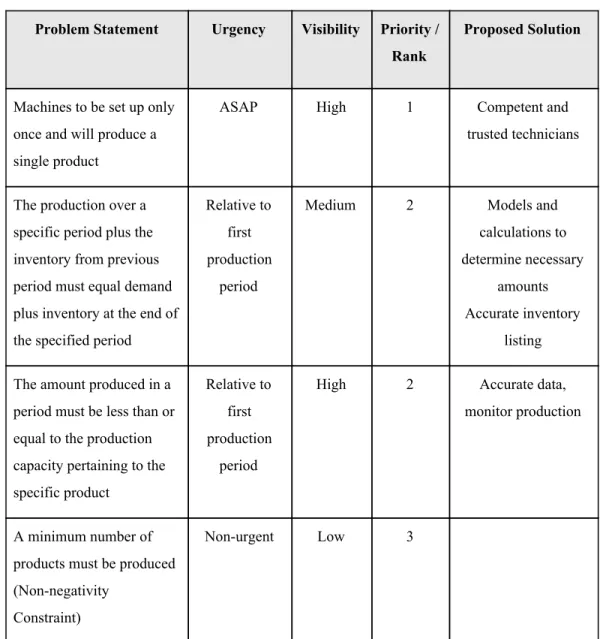
3.1.2 PROBLEM STATEMENT

Problem Statement Urgency Visibility Priority / Rank

Proposed Solution

Machines to be set up only once and will produce a single product

ASAP High 1 Competent and

trusted technicians

The production over a specific period plus the inventory from previous period must equal demand plus inventory at the end of the specified period

Relative to first production

period

Medium 2 Models and

calculations to determine necessary

amounts Accurate inventory

listing The amount produced in a

period must be less than or equal to the production capacity pertaining to the specific product

Relative to first production

period

High 2 Accurate data,

monitor production

A minimum number of products must be produced (Non-negativity

Constraint)

Non-urgent Low 3

(14)

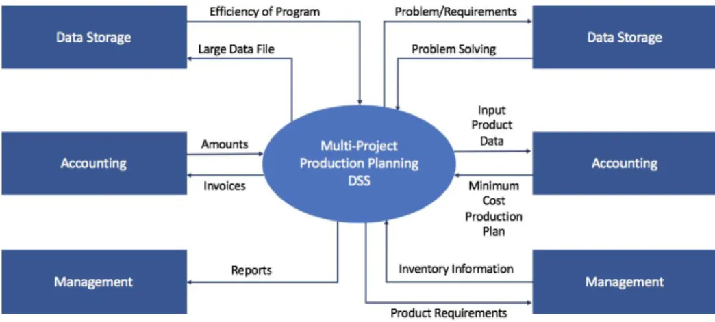
3.1.3 CONTEXT DIAGRAM

The System Context Diagram displays how the external environment and the system interact.

Figure 2: Context Diagram

3.2 SYSTEMS ANALYSIS

Systems analysis defines the problems to be solved and provides a design of a system to solve the problem.The first step in systems analysis is determining the problem, and then analyze the problem. In this problem there are three objectives and five constraints given. All of these aspects of the problem had to be analyzed thoroughly in order to create a final solution. The objective of the problem is to find a way to minimize the production costs, holding costs, and setup costs. When completing these objectives the constraints must also be kept in mind, when solving this problem. The constraints are: In each time period machines will be set up once and a single

prod_{uct will be produced, the flow conservation constraints show that the production}

in a particular period plus the inventory from the last period should be equal to the demand plus the inventory at the end of the period, the amount of product produced in the period should be less than or equal to production capacity for this product, and finally the last constraint is non negativity.

(15)

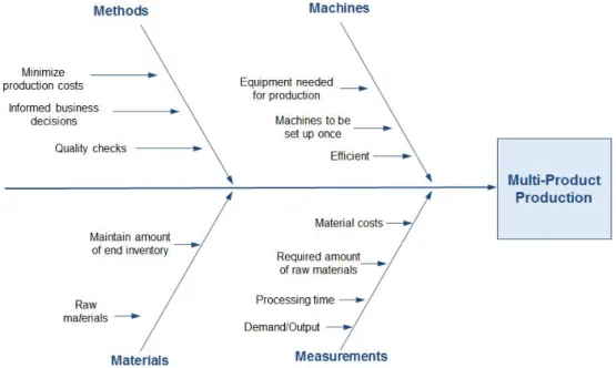
3.2.1 FISHBONE DIAGRAM

The Fishbone Diagram is a tool that is used for categorizing the causes of a problem in order to identify its root causes.

Figure 3: Fishbone Diagram

3.2.2 REQUIREMENT ANALYSIS

The Requirement Analysis is the process of determining user expectations for a new or modified product or system. The requirement analysis helps

determine the needs and conditions that must be met in order for the system to succeed. This analysis is critical to the success of a development project. The requirements which are determined must be actionable, measurable, testable, related to identified business needs or opportunities, and defined to a level of detail sufficient for system design. The following are the requirements which are applicable for this Decision Support System:

● Functional Requirements

○ These are the requirements which must be identified in order to complete the task.

(16)

■ The end inventory matches the previous period

■ Minimize the production costs

■ Minimize the inventory holding costs

■ Minimize the setup costs

■ Completes objectives

■ Attains to constraints

■ Effective and accurate decision support system

● Non-functional Requirements

○ These are the requirements that judge the operation of the system.

○ The non-functional requirements are:

■ Easy-to-use user interface

■ Performance

■ Easy to learn how to operate the system

■ Aesthetically pleasing to the user

■ Quality

■ Coverage

■ Timeliness

■ Design Requirements

3.2.3 LOGICAL DESIGN

Logical models reduce the risk of missing business requirements because often people are too preoccupied with technical results, they also allow the DSS creator to communicate with end-users in less technical languages. One of the ways to display the logical design on this system is through a Data Flow Diagram (DFD). The DFD shows the flow of data through the system. Another way to show the logical design of this system is through a use case diagram. The use case diagram depicts the event steps typically defining the interactions between a role and a system to achieve a goal.

(17)

Figure 4: Use Case Diagram

(18)

3.3 SYSTEM DESIGN

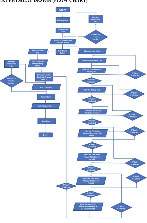
3.3.1 PHYSICAL DESIGN (FLOW CHART)

(19)

3.4 SYSTEM IMPLEMENTATION & CONSTRUCTION

3.4.1 USER INTERFACE: FORMS AND INPUT SHEETS

Forms were used in this DSS in order to help input the data for the user. Figure 7 displays the welcome form. Once the system opens, this is the first form which pops up onto the screen. The form has the company logo and welcomes the user to the DSS and prompts the user to continue.

Figure 7: Welcome Form

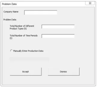
Once the user clicks on the “Click to Continue” button, they will be prompted by the “Problem Data Form” (Figure 8). This form allows the user to input the company name in addition to the values for the number of products and time periods. The form then has the option for the user to manually enter the data into Excel or for the data to be read from an existing file.

(20)

Figure 8: Problem Data Form

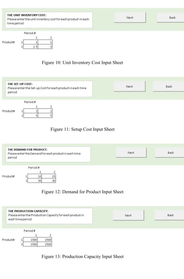
Once the user clicks on the “Accept” button, then the user will be brought to an Excel sheet (Figure 9). This sheet will prompt the user to enter the

production unit costs. The matrix for the amount of products and periods will already be outlined from the data which was inputted into the problem data form (Total number of products and the total number of time periods). Once the user clicks on the “Next” button, they will be brought to the next sheet where they will need to input the unit inventory costs (Figure 10). The matrix will again automatically by outlined for the user. If the user selects the “Back” button, they will be brought back to the previous sheet they were on. The same procedure will continue for the set-up costs (Figure 11), the demand for

product (Figure 12), and the production capacity (Figure 13). On this DSS there will only be one sheet open at a time. Once the user clicks the next button a new sheet appears and the previous one is hidden.

(21)

Figure 10: Unit Inventory Cost Input Sheet

Figure 11: Setup Cost Input Sheet

Figure 12: Demand for Product Input Sheet

(22)

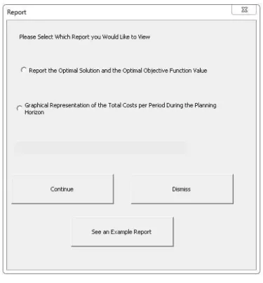
Once the user clicks on the “Next” button on the production capacity input form, the user will be prompted with the “Report Form” (Figure 14). This form allows the user to choose which solution report they would like to view. Once they click continue the corresponding report tab will open. If the user would like to see an example report, they can do so by clicking the button “See an Example Report”. Then the user will be prompted by another form, the “Example Report Form” (Figure 15). Here they will be able to choose which sample report they would like to view. Once the user chooses a report and then clicks the “Continue” button the corresponding report will open on an Excel sheet.

(23)

Figure 15: Example Report Form

Figure 16 and Figure 17 show the example reports which will appear when the user selects to see the example report. Figure 16 is the Example Report, which represents the Optimal Solution and the Optimal Objective Value there are pre-made matrixes on the sheet which represent what the user has filled in already, and they will be able to see the solution to the problem using those numbers. Figure 17 is Example Report , this report gives a graphical

representation of the total costs per period during the planning horizon. This report uses the same values in example report in Figure 16. If the user clicks the “Back to Report Options” button on either report sheet, they will be returned to the “ Report From”

(24)

Figure 16: Example Report #1 (Optimal Solution and the Optimal Objective Value)

Figure 17: Example Report #2 (Graphical representation of the total costs per period during the planning horizon)

3.4.2 SOURCE CODE

The VBA code in this DSS is intended to make the experience of using the software very simple for the user. Figure 18 is the sub procedure which is connected to the “click to continue” button on the “Welcome Form”. This procedure hides all sheets not currently in use, then displays and activates the sheet associated with that form. This helps to make the DSS more user friendly by displaying only one sheet at a time.

(25)

Figure 18: Welcome Form Code

Figure 19 is the module that will create the tables on each Excel sheet

(according to the number or products and the number of time periods entered by the user). First it clears the contents of the page, then creates the matrix. This sub procedure is then called into each sheet when the user clicks the “Next Button”, this can be seen in Figure 20 and 21.

(26)

Figure 19: Make Table

Figure 20 is the sub procedure connected to the “Accept” button on the “Problem Data Form”. When this button is clicked it initializes both product number and period number and assigns the respective values. It then hides the previous sheet and displays/activates the sheet related to this form. The sub procedure also calls the “MakeTable” sub procedure (Figure 19).

(27)

The “Next” and “Back” buttons are on every sheet, Figure 20 is an example of the sub procedures behind the buttons on one of the sheets. As stated before, this procedure hides all sheets not currently in use and then displays and activates the sheet associated with that form. This helps to make the DSS more user friendly by displaying only one sheet at a time.

Figure 21: Next and Back Buttons

Figure 21 and Figure 22 represent the code for the “Report Form” and the “Example Report Form”. These sub procedures allow the user to select which report they would like to view and the corresponding report sheet will open.

(28)

Figure 22: Report Options

Figure 23: Example Report Options

In Report #1 (Optimal Solution and the Optimal Objective Value), the user will need to run Solver in order to obtain a final solution. All the user will

(29)

page which will run the solver. Figure 24 displays the program used to complete this task.

Figure 24: Run Solver

3.4.3 LEVEL OF AUTOMATION USING VBA

In this DSS there will only ever be one sheet open at a time, there is a sub procedure that hides all sheets not currently in use, then displays and activates the sheet associated with that form. This helps to make the DSS more user friendly by displaying only one sheet at a time. The user will not have to worry about changing the input values for the parameters, as there are “Next” and “Back” buttons on each sheet. This allows the users to go back and forth without any trouble. The results are all automatically calculated. In Report #1 (Optimal Solution and the Optimal Objective Value) the user does not need to enter any values into the solver, or make any constraints. This is all done for them. All the user needs to do is click the button “Solve for Optimal Solution” in order to receive the results. Also for Report #2 (Graphical representation of the total costs per period during the planning horizon), the graph is

(30)

4. RESULTS

Below are photos of the results of the Decision Support System. These results are based off of the values that the user had previously inputted for the problem parameters. Figure 25 and Figure 27 show the 2 reports of the final solution for the users problem. (The source data is in Figures 9-13). Figure 26 shows the constraints which are in the solver system. These

constraints help determine the final answer. The calculated results represent a minimum cost production plan specific to the users specified parameters.

Figure 25: Report #1 (Optimal Solution and the Optimal Objective Value)

Figure 26 displays the constraints that solver will apply to solve the production problem. Here the user can manage and edit the different constraints, set the objective function to max or min and also choose the desired solving method. After selecting the desired options and clicking solve, the system will present the user with a minimum cost production plan corresponding to the data they have entered into the DSS.

(31)

Figure 26: Solver Parameters for Report #1

Figure 27 displays a graphical representation of the total incurred costs over a time period. The values calculated using solver are also displayed in tables beside the graph, these values correspond to the points on the graph. The three displayed costs are production cost,

inventory holding cost and setup cost which are based on the production data previously entered by the user.

(32)

Figure 27: Report #2 (Graphical representation of the total costs per period during the planning horizon)

(33)

6. DISCUSSION

This DSS is able to determine the least cost production plan that will satisfy the end user. It determines the best use of scarce resources in order to meet the customer’s demand at the least possible cost. The results which were obtained are extremely accurate, and the Solver system is all automated, which means the user does not need to solve anything independently.

The main objective of this project was to better comprehend the phases of developing a Decision Support System. Many challenges were faced while completing this project. These challenges enhanced the already known skills and knowledge about DSS’s. One of the biggest tasks that our team faced was determining where to begin. After a basic example was developed using small values for the various parameters, it became more clear how to start formulating the problem on Excel. Linear programming (LP) concepts were used to

determine how to create the DSS. Once the minimization equation (objective function) and the associated constraints were determined, the LP concepts were applied to formulate and solve the problem in Excel’s Solver application.

One of the best aspects about the DSS is the users interaction with the system. The system is extremely easy to use. Only one sheet is open at all times, in order to not confuse the users with an abundance of Excel sheets. Also, the system is highly automated, so the users only need to enter their data for the required parameters and do not have to solve anything by themselves.

Throughout the project the greatest difficulties were experienced when trying to formulate and solve the problem with Excel’s Solver tool. Further knowledge of and practice with, this application is required to solve problems of this degree of difficulty. The main weakness of this system is that the end user is still required to input several values associated with the production data. In the case of a production plan that involves manufacturing many different products the amount of input data needed could be quite large thus becoming a very tedious task for the user. One such situation where this system can be applied is to determine the best use of scarce resources in order to minimize production costs yet still satisfy the customer’s

(34)

7. CONCLUSION

Overall, this project is extremely realistic. Many Industrial Engineers work on the optimization of multi product production, which is exactly what this project displayed. It helped our team fully understand all of the aspects which need to be taken into account when finding the optimum solution for a production facility. This project also served the purpose of creating a real world scenario. These crucial deadlines create a sort of workplace atmosphere during the project. Being given a task that is fully in your hands, from start to finish, was great practice for future tasks that any Industrial Engineering student may have to take on as a professional engineer in the workplace.

(35)