Spatial and Temporal Diffusion of
House Prices in the UK
Sean Holly
M. Hashem Pesaran
Takashi Yamagata
CES
IFO
W
ORKING
P
APER
N
O
.
2913
CATEGORY 12: EMPIRICAL AND THEORETICAL METHODS
JANUARY 2010
An electronic version of the paper may be downloaded • from the SSRN website: www.SSRN.com • from the RePEc website: www.RePEc.org • from the CESifo website: Twww.CESifo-group.org/wpT
CESifo Working Paper No. 2913
Spatial and Temporal Diffusion of
House Prices in the UK
Abstract
This paper provides a method for the analysis of the spatial and temporal diffusion of shocks in a dynamic system. We use changes in real house prices within the UK economy at the level of regions to illustrate its use. Adjustment to shocks involves both a region specific and a spatial effect. Shocks to a dominant region - London - are propagated contemporaneously and spatially to other regions. They in turn impact on other regions with a delay. We allow for lagged effects to echo back to the dominant region. London in turn is influenced by international developments through its link to New York and other financial centers. It is shown that New York house prices have a direct effect on London house prices. We analyse the effect of shocks using generalised spatio-temporal impulse responses. These highlight the diffusion of shocks both over time (as with the conventional impulse responses) and over space.
JEL-Code: C21, C23.
Keywords: house prices, cross sectional dependence, spatial dependence.
Sean Holly Faculty of Economics University of Cambridge [email protected] M. Hashem Pesaran Faculty of Economics University of Cambridge [email protected] Takashi Yamagata
Department of Economics and Related Studies University of York
December 2009
We are grateful to Alex Chudik, Chris Rogers, Ron Smith, Elisa Tosetti, and participants in the Cambridge Finance Workshop for helpful comments where a preliminary version of this paper was first presented.
1
Introduction
This paper provides a method for the analysis of the spatial and temporal di¤usion of shocks in a dynamic system. We use changes in real house prices within the UK economy at the level of regions to illustrate its use. Adjustment to shocks involves both a region speci…c and a spatial e¤ect. Shocks to a dominant region - London - are propagated contemporaneously and spatially to other regions. They in turn impact on other regions with a delay. We allow for lagged e¤ects to echo back to the dominant region. London in turn is in‡uenced by international developments through its link to New York and other …nancial centers. We analyse the e¤ect of shocks using generalised spatio-temporal impulse responses. These highlight the di¤usion of shocks both over time (as with the conventional impulse responses) and over space.
The present paper provides a relatively simple and consistent approach to modelling spatial and temporal adjustments quantitatively.1 We approach the analysis from the
perspective of recent developments in the literature on panel data models with a spatial dimension that manifests itself in the form of cross sectional dependence. One of the most important forms of cross section dependence arises from contemporaneous dependence across space and this is the primary focus of the spatial econometrics literature. This spatial dependence (Whittle, 1954) approach models correlations in the cross section by relating each cross section unit to its neighbour(s). Spatial autoregressive and spatial error component models are examples of such processes. (Cli¤ and Ord, 1973, Anselin, 1988, Kelejian and Robinson, 1995, Kelejian and Prucha, 1999, 2009, and Lee, 2004). Proximity, of course, does not have to be limited to proximity in space. Other measures of distance such as economic (Conley, 1999, Pesaran, Schuermann and Weiner, 2004), or social distance (Conley and Topa, 2002) could also be employed. In a regional context proximity of one region to another can depend on transport infrastructure. The ability to commute easily between two areas is likely to be a much better indication of economic inter-dependence than just physical closeness.2
Another approach to dealing with cross sectional dependence is to make use of mul-tifactor error processes where the cross section dependence is characterized by a …nite number of unobserved common factors, possibly attributable to economy-wide shocks that a¤ect all units in the cross section, but with di¤erent intensities. With this ap-proach the error term is a linear combination of a few common time-speci…c e¤ects with heterogeneous factor loadings plus an idiosyncratic (individual-speci…c) error term. Pe-saran (2006) has proposed an estimation method that consists of approximating the linear combinations of the unobserved factors by cross section averages of the dependent and explanatory variables and then running standard panel regressions augmented with the cross section averages. An advantage of this approach is that it yields consistent estimates even when the regressors are correlated with the factors, and the number of factors are unknown. A maximum likelihood procedure is also suggested by Bai (2009).
1The way in which space and time interact has long been a primary concern of epidemiologists and
regional scientists. For a qualitative analysis of spatio-temporal processes using geographical information systems, see Peuquet (1994). However, there is also widespread interest in the environmental sciences as well. For a recent contribution see, for example, Kneib and Fahrmeir (2009). The study of the human brain through the use of magnetic resonance imaging also involves spatial-temporal modeling. See, for example, Gössl et al. (2001), and Fahrmeir and Gössl (2002).
2At the industry level interdependency between industries and …rms are more likely to re‡ect patterns
of intermediate input usage rather than physical proximity. See Horvath (1998, 2000) and Holly and Petrella (2008).
More recently Pesaran and Tosetti (2009) have sought to combine the insights of these two approaches and propose a panel model in which the errors are a combination of a multifactor structure and a spatial process. To achieve this a distinction is drawn between what is termed weak and strong cross section dependence. (Chudik, Pesaran and Tosetti, 2009). A process is said to be cross sectionally weakly dependent at a given point in time, if its weighted average at that time converges to its expectation in quadratic mean, as the cross section dimension is increased without bounds. If this condition does not hold, then the process is said to be cross sectionally strongly dependent. The distinctive feature of strong correlation is that it is pervasive, in the sense that it remains common to all units however large the number of cross sectional units. Signi…cantly, spatial dependence typically entertained in the literature turns out to be weakly dependent in this framework. Holly, Pesaran and Yamagata (2009) model house prices at the level of US States where there is evidence of signi…cant spatial dependence even when the strong form of cross sectional dependence has been swept up by the use of cross sectional averages. If we were to extend the sample by including regions or countries in Europe we would still expect that the spatial e¤ects of New York State would be con…ned to its neighbouring states and not extend to Europe. By contrast common factors coming from the aggregate US economy could still have pervasive e¤ects for regions of Europe.
As compared to purely spatial or purely factor models analysed in the literature, the spatio-temporal model estimated in this paper uses London house prices as the common factor and then models the remaining dependencies (contemporaneously or with a lag) conditional on London house prices. This allows us to consistently estimate separate conditional error correcting models for the di¤erent regions in the UK, which we then combine with a model for London to solve for a full set of spatio-temporal impulse response functions. Two alternative speci…cations are considered for London house prices, one speci…cation that only depends on lagged London and neighbouring house price changes, and another which also depends on New York house prices.
While we are able to demonstrate that London is a dominant region for the rest of the UK, it is not immediately obvious why it should be uniquely so. One possibility we consider is that London is the largest city in Europe but more signi…cantly is a major world …nancial centre. Developments in world …nancial markets can impact directly on the London housing market. Because London’s traditional role as a …nancial and trading centre and the attraction that it has for economic migration of highly skilled workers, residential prices re‡ect both local factors in the UK but also movements abroad. In particular, there is a well established international market in residential property in which London along with New York plays a role. Our test results clearly show that New York house prices are signi…cant drivers of house prices in the UK, but only through London. We also explored the possibility that Paris house prices could be one of the drivers of London house prices but found little evidence in its support.
It is important to note that the focus of our analysis di¤ers from many others where the intention is to understand what determines regional house prices in terms of income, housing costs and other …xed factors to explain di¤erences in regional house prices.3 Al-though our approach does not preclude the inclusion of observable covariates such as incomes and interest rates we have focussed on the dispersion of house price shocks, con-ditioning on a dominant region (London) and neighbourhood e¤ects, so the formulation is particularly parsimonious. It can be seen as a …rst step towards a more structural
under-3See, for example, Ashworth and Parker (1997), Cameron and Muellbauer (1998), Gallin (2006), and
standing of the inter-play of house price di¤usion and the evolution of the real economy nationally and regionally.4
There have been a number of other studies that have considered the spatial di¤usion of house prices. One of the …rst was Can (1990). He studied what he calls ‘neighbourhood dynamics’by using a hedonic model of house prices where the price of a house depends on a series of characteristics, and incorporates both spatial spillover e¤ects and spatial parametric drift. More recently Fingleton (2008) has developed a GMM estimator for a spatial house price model with spatial moving average errors. However, both of these studies con…ne themselves to the cross section dimension and do not consider the adjust-ment of prices over time. Studies of house prices that do consider both dimensions are van Dijk et al. (2007) and Holly et al. (2009). These studies develop a model that al-lows for stochastic trends, cointegration, cross-equation correlations and the latent-class clustering of regions. Dijk et al. apply their model to regional house prices in the Nether-lands. They pick up a ‘ripple’ e¤ect, by which shocks in one region are propagated to other regions. Holly et al. consider the evolution of real house prices and real disposable incomes across the 48 U.S. States and after allowing for unobserved common factors …nd statistically signi…cant evidence of autoregressive spatial e¤ects in the residuals of the cointegrating relations. Chudik and Pesaran (2009a) show that signi…cant improvements in …t is achieved if Holly et al.’s regressions are augmented with spatially weighted cross sectional averages.
Conventional impulse response analysis traces out the e¤ect of a shock over time. However, with a spatial dimension as well, dependence is both temporal and spatial (Whittle, 1954). Our results suggest that the e¤ects of a shock decay more slowly along the geographical dimension as compared to the decay along the time dimension. For example, the e¤ects of a shock to London on itself, die away and are largely dissipated after two years. By contrast the e¤ects of the same shock on other regions takes much longer to dissipate, the further the region is from London. This …nding is in line with other empirical evidence on the rate of spatial as compared to temporal decay discussed in Whittle (1956), giving the examples from variations of crop yields across agricultural plots, ‡ood height and responses from population samples.
The rest of the paper is set out as follows: In Section 2 we propose a model of house price di¤usion where we distinguish between the dominant and the non-dominant regions. In Section 3 we show how the individual models of regional house prices that have been treated separately for estimation purposes can be brought together and used for impulse response analysis along the time as well as the spatial dimensions. We also consider an extension of the basic model to allow for the e¤ects of external shocks in the form of New York house prices. In Section 4 we report some empirical results using quarterly regional real house price data for the UK over the period 1974q1-2008q2. Finally, in Section 5 we
4Another branch of the literature explores the transmission of shocks in real estate markets including
both residential and commercial property both within countries and across national borders. For example, Case et al. (2000) show that correlations between international real estate markets are high, given the degree to which they are segmented. They attribute a substantial amount of the correlation across world property markets to GDP which is correlated across countries. Herring and Wachter (1999) have pointed out that the 1997 Asian crisis was characterized by a collapse in real estate prices and a consequent weakening of the banking system before exchange rates came under attack. The essential link was that the real estate collapse impacted very negatively on the balance sheets of banks. Herring and Wachter point to a strong correlation between real estate cycles and banking crisis across a wide variety of countries. Bond, Dungey and Fry (2006) have also considered the transmission of real estate shocks during the East Asian crisis and the role they played in …nancial contagion.
draw some conclusions.
2
A Price Di¤usion Model
Suppose we are interested in the di¤usion of (log) prices,pit, over time and regions indexed
by t = 1;2; :::; T and i = 0;1; :::; N and we have a priori reason to believe that one of the regions, say region 0, is dominant in the sense that shocks to it propagate to other regions simultaneously and over time, whilst shocks to the remaining regions has little immediate impact on region0, although we do not rule out lagged e¤ects of shocks from regions i = 1;2; ::; N to region 0. This is an example of a ‘star’ network within which each region can be viewed as a node. A …rst order linear error correction speci…cation is given by5
p0t= 0s(p0;t 1 ps0;t 1) +a0+a01 p0;t 1+b01 ps0;t 1+"0t (2.1)
and for the remaining regions
pit = is(pi;t 1 psi;t 1) + i0(pi;t 1 p0;t 1) +ai
+ai1 pi;t 1 +bi1 pi;ts 1+ci0 p0t+"it; (2.2)
for i= 1;2; :::; N. ps
it denotes the spatial variable for region i de…ned by
psit = N X j=0 sijpjt, with N X j=0 sij = 1; for i= 0;1; :::; N: (2.3)
The weights sij 0 can be set a priori, either based on regional proximity or some
economic measure of distance between regions i and j. In the empirical application we use a contiguity measure where sij is equal to 1=ni if i and j share a border and zero
otherwise, withni being the number of neighbors ofi. psit can be viewed as a local average
price for regioni. The weightssij can be arranged in the form of a spatial matrix,S, which
is row-standardized, namelyS N+1= N+1, where N+1 is an(N+ 1) 1vector of ones.
Note also that whenS captures contiguity measures its column norm will be bounded in
N, namely that Ni=0 sij < K, for all j; and as shown in Chudik and Pesaran (2009b),
conditional on the dominant unit the remaining spatial dependence will be weak and conditional (on London) pair-wise dependence of the regions vanishes ifN is su¢ ciently large.
The price equations are allowed to be error correcting, although whether they are is an empirical issue. In principle, the speci…cation of the error correcting equations depends on the number of the cointegrating relations that might exist amongst the house prices across theN+1regions. To avoid over-parametrization in the above speci…cations we have opted for relatively parsimonious speci…cations where London prices are assumed to be cointegrating with the average prices in the neighbourhood of London,ps
0t, whilst allowing
for prices in other regions to cointegrate with London as well as with the neighbouring regions. In the case where prices cointegrate across all pairs of regions with the coe¢ cients
(1; 1);it is easily seen that prices of each region must also cointegrate with prices of the neighbouring regions. It is interesting to note that the reverse is also true, namely if prices in each region cointegrate with prices of the neighbouring regions with the coe¢ cients
(1; 1), then all price pairs would be cointegrating. Our error correcting speci…cations can therefore be justi…ed as a parsimonious representation of pair-wise cointegration of prices across regions. The empirical validity of such an approximation for modelling of regional house prices in the UK will be investigated below.
Finally, note that the price change in the dominant region, p0t, appears as a
con-temporaneous spatial e¤ect for the ith region. But there is no contemporaneous local average price included in the equation for p0t. Implicit in the above speci…cation is
that conditional on the dominant region’s price variable and lagged e¤ects the shocks,
"it, are approximately independently distributed across i. The assumption that p0t, is
weakly exogenous in the equation pit, i= 1;2; :::; N can be tested using the procedure
advanced by Wu (1973), which can also be motivated using Hausman’s (1978) type tests. Following Wu’s approach denote the OLS residuals from the regression of the model for the dominant region by
^
"0t= p0t ^0s(p0;t 1 ps0;t 1) ^a0 a^01 p0;t 1 ^b01 ps0;t 1;
and run the auxiliary regression
pit = is(pi;t 1 psi;t 1) + i0(pi;t 1 p0;t 1) (2.4)
+ai+ai1 pi;t 1+bi1 psi;t 1+ci0 p0t+ i^"0t+ it;
and use a standard t-test to test the hypothesis that i = 0 in this regression (for each i
separately). This test is asymptotically equivalent to using Hausman’s procedure which involves testing the statistical signi…cance of the di¤erence between the OLS and the IV estimates of (ai; ai1; bi1; ci0), using p0;t 1 and ps0;t 1 as instruments for p0t in (2.2).
It is clear that the test can only be computed if the instruments are not already included amongst the regressors of the model for the non-dominant regions. In our set up this is satis…ed ifN >1. WhenN = 1; ps
0;t 1 = p1;t 1, and ps1;t 1 = p0;t 1 and the model
reduces to a bivariate VAR in p0t and p1t.
3
Spatio-temporal Impulse Response Functions
Although the regional price model can be de-coupled for estimation purposes, for simula-tion and forecasting the model represents a system of equasimula-tions that needs to be solved simultaneously. We begin by writing the system of equations in (2.1) and (2.2) as
pt =a+Hpt 1+(A1+G1) pt 1+C0 pt+"t; (3.5) where pt= (p0t; p1t; :::; pN t)0, a= (a0; a1; :::; aN)0,"t= ("0t; "1t; :::; "N t)0, H= 0 B B B B B @ 0s 0 0 0 10 1s+ 10 0 0 0 .. . ... . .. ... ... N 1;0 0 N 1;s+ N 1;0 0 N0 0 0 N s+ N0 1 C C C C C A 0 B B B B B @ 0ss00 1ss01 .. . N 1;ss0N 1 N ss0N 1 C C C C C A A1 = 0 B B B B B @ a01 0 0 0 0 a11 0 0 0 .. . ... . .. ... ... 0 0 aN 1;1 0 0 0 0 aN1 1 C C C C C A ; G1 = 0 B B B B B @ b01s00 b11s01 .. . bN 1;1s0N 1 bN1s0N 1 C C C C C A ; C0 = 0 B B B B B @ 0 0 0 0 c10 0 0 0 0 .. . ... . .. ... ... cN 1;0 0 0 0 cN0 0 0 0 1 C C C C C A ;
where s0
i = (si0; si1; :::; siN). Recall that s0i N+1 = 1. It is therefore, easily veri…ed that
H N+1 = 0, and hence H is rank de…cient. From this it also follows that one or more
elements of the price vector,pt, must have a unit root.
Solving for price changes we have
pt = (IN+1 C0) 1a+ (IN+1 C0) 1 pt 1 +(IN+1 C0) 1(A1+G1) pt 1+ (IN+1 C0) 1"t; pt= + pt 1+ pt 1+R"t; (3.6) where = Ra; with R= (IN+1 C0) 1; = RH, =R(A1 +G1). (3.7)
Since R is a non-singular matrix it follows that and H have the same rank, and will also be rank de…cient ( N+1 = RH N+1 = 0). Therefore, (3.6) represents a
system of error correcting vector autoregressions in pt. The number of cointegrating or long run relations of the model depends on the rank of H(or ). The underlying price speci…cations in (2.1) and (2.2) imply the possibility of at mostN cointegrating relations. For example, if all regional house prices were cointegrated with prices in London, then we will haveN cointegrating relations. In what follows we denote the number of cointegrating relations byr(0 r N), and write = 0where and are(N+1) rfull column rank matrices. The choice of r is an empirical issue to which we shall return to below.
To examine the spatio-temporal nature of the dependencies implied by (3.6) we …rst write it as a vector autoregression (VAR)
pt = + 1pt 1+ 2pt 2+R"t (3.8)
where 1 = (IN+1+ 0+ ), and 2 = . The temporal dependence of house prices
is captured by the coe¢ cient matrices 1 and 2, and the spatial dependence by R and
the error covariances, Cov("it; "jt) for i6=j. The temporal coe¢ cients in 1 and 2 are
also a¤ected by the spatial patterns in the regional house prices as we have constrained the lagged e¤ects and the error correction terms to match certain spatial patterns as characterized by the non zero values of sij. The above VAR model can now be used for
forecasting or impulse response analysis.
For impulse response analysis it is important to distinguish between two types of counterfactuals. Assuming that the Wu test of the weak exogeneity of p0tis not rejected,
then it would be reasonable to assume that Cov("0t; "it) = 0; for i = 1;2; :::; N. In this
case the impulse responses of a unit (one standard error) shock to house prices in the dominant region on the rest of regions at horizonh periods ahead will be given by
g0(h) = E(pt+hj"0t =p 00;It 1) E(pt+hjIt 1)
= p 00 hR e0; for h= 0;1; :::; (3.9)
where It 1 is the information set at time t 1, 00 =V ar("0t),e0 = (1;0;0; :::;0)0, and
h = 1 h 1+ 2 h 2;for h= 0;1; :::; (3.10)
with the initial values 0 =IN+1, and h =0, forh <0.6 6See also Chapter 6 in Garratt et al. (2006).
To derive the impulse responses of a shock to non-dominant regions we need to allow for possible contemporaneous correlations across the regions i and j for i; j = 1;2; :::; N. This can be achieved using the generalized impulse response function advanced in Pesaran and Shin (1998). In the present application we would have
gi(h) =
hR ei
p
ii
; for h= 0;1; :::; H (3.11)
where ei is an(N + 1) 1 vector of zeros with the exception of its ith element which is
unity, = 0 B B B B B B B @ 00 0 0 0 0 0 11 12 1;N 1 1N 0 21 22 2;N 1 2N .. . ... ... . .. ... ... 0 N 1;1 N 1;2 N 1;N 1 N;N 1 0 N1 N2 N 1;N N N 1 C C C C C C C A ; (3.12)
where ij = E("it"jt). The elements of can be estimated consistently from the OLS
residuals,^"it of the regressions for the individual regions, namely by, ^ij =T 1 Tt=1^"it^"jt,
for i; j = 1;2; :::; N, and ^00 =T 1 Tt=1^"0t^"0t. With the above speci…cation of , where
its …rst row and column are restricted, gi(h) =
1=2
ii hR ei = g0(h) for i= 0: So the
generalized impulse response function (GIRF) de…ned by (3.11) with given by (3.12) is applicable to the analysis of shocks to the dominant and non-dominant regions alike. The distinction between the two types of regions is captured by the zero-bordered form of . The recursive nature of the model with London as the dominant unit identi…es the e¤ects of shocks to London house prices. But due to the non-zero correlation of shocks across the remaining regions the e¤ects of shocks to region i6= 0 is not identi…ed.
It is worth noting that
R= (IN+1 C0) 1 = 0 B B B B B @ 1 0 0 0 c10 1 0 0 0 .. . ... . .. ... ... cN 1;0 0 1 0 cN0 0 0 1 1 C C C C C A : (3.13)
Also since sii= 0, we have
A1+G1 = 0 B B B B B @ a01 b01s01 b01s0;N 1 b01s0N b11s10 a11 b11s1;N 1 b11s1N .. . ... . .. ... ... bN 1;1sN 1;0 bN 1;1sN 1;1 aN 1;1 bN 1;1sN 1;N bN1sN0 bN1sN1 bN1sN;N 1 aN1 1 C C C C C A ; (3.14)
and recalling that N
j=0sij = 1, thenkA1+G1kr= maxi(jai1j+jbi1j)< K, andkA1+G1kc =
maxj jaj1j+ Ni=0jbi1jsij which is also bounded in N since Ni=0sij < K, and jai1j and
jbi1j are bounded inN; by assumption.7
7kAk
In the context of the IVAR model discussed in Pesaran and Chudik (2009a,b), the spatio-temporal aspects of the underlying di¤usion process are characterized by the co-e¢ cient matrices R, ; 1 and 2. In the present application, due to the dominance of
region 0, we have
kRkc = 1 + Ni=1jci0j=O(N); (3.15)
and the column norm of R is unbounded in N. As shown in Pesaran and Chudik the dominant region can be viewed as a common factor for the other regions, and conditional on p0t, the cross dependence of pit across i = 1;2; :::; N will be weak and not allowing
for it at the estimation stage can only a¤ect e¢ ciency which will become asymptotically negligible when N is su¢ ciently large.
In cases where N is relatively small (as in the empirical application that follows), the estimation of the conditional models will be less e¢ cient as compared to the full maximum likelihood estimation, treating all the equations of the model simultaneously. But such an estimation strategy is likely to be worthwhile only if N is really small, say 5 or 6. Even for moderate values of N the number of parameters to be estimated can be quite large compared to T (the time dimension) which could adversely a¤ect the small sample properties of the maximum likelihood estimates.
Also, one can clearly generalize the model by introducing other (observed) national or international factors into the equation for the dominant region such as real disposable income (which need not be region speci…c), interest rates, or house prices in the US or Europe. In this paper we shall only consider the e¤ects of New York house prices, and leave other extensions of the model to future research.
3.1
The Price Di¤usion Model with Higher Order Lags
For higher lag order processes, the model of the dominant region is given by
p0t= 0s(p0;t 1 ps0;t 1) +a0+ k X `=1 a0` p0;t `+ k X `=1 b0` ps0;t `+"0t (3.16)
and for the remaining regions by
pit = is(pi;t 1 psi;t 1) + i0(pi;t 1 p0;t 1) (3.17)
+ai+ k X `=1 ai` pi;t `+ k X `=1 bi` psi;t `+ k X `=0 ci` p0;t `+"it;
for i = 1;2; :::; N. Combining (3.16) and (3.17), the full system of equations can be written as pt=a+Hpt 1+ k X `=1 (A`+G`) pt `+ k X `=0 C` pt `+"t: (3.18)
Solving for price changes we have
pt = + pt 1+
k
X
`=1
` pt `+R"t; (3.19)
where =Ra with R= (IN+1 C0) 1; =RH, as before, and
Writing (3.19) as a VAR in price levels pt = + k+1 X `=1 `pt `+R"t; (3.20)
where 1 =IN+1+ + 1, ` = ` ` 1 for `= 2; :::; k, and k+1 = k.
The generalised impulse response function for the ith region at horizon h is the same as before and is given by (3.11), except that h must now be derived recursively using
the following generalization of (3.10):
h = k+1
X
`=1
` h `; for h= 0;1; :::; (3.21)
with the initial values 0 =IN+1, and h =0, forh <0.
Note that the equations (3.16) and (3.17) could have di¤erent lag-orders for each terms for each region, kia, kib, kic, say. In the empirical section, we consider the case
in which these lag-orders are selected by an information criteria (IC), such as Akaike IC (AIC) and Schwarz Bayesian Criterion (SBC). The heterogeneity of the lag orders across regions and variable type can be accommodated by de…ning k = maxifkia; kib; kicg; and
then setting to zero all the lag coe¢ cients that are shorter than k.
3.2
Bootstrap GIRF Con…dence Intervals
As is well known the asymptotic standard errors of the estimated impulse responses are likely to be biased in small samples. There is also the possibility of non-Gaussian shocks that ought to be taken into account in small samples. For both of these reasons we compute bootstrapped con…dence intervals for the estimates of gi(h), over h and i, to
evaluate their statistical signi…cance.
To this end denote the estimated model of (3.20) as pt = ^+ `k=1+1^`pt `+R^^"t,
and the estimated GIRF as bgi(h) = ^hR ^ e^ i=
p
^ii. We generate B bootstrap samples
denoted byp(tb); b = 1;2; :::; B, then compute bootstrap GIRFbgi(b)(h)for eachp(tb). Firstly, thebth bootstrap samples are obtained recursively based on the DGP
p(tb) =^+ k+1 X `=1 ^ `p (b) t `+R^^" (b) t ; (3.22) where "(tb) = ^1=2 (b)
t , where the elements of
(b)
t are random draws from the
trans-formed residual matrix, ^ 1=2(^"
1;^"2; :::;^"T), with replacement. The k+ 1 initial
obser-vations are equated to the original data.
Secondly using the obtained bootstrap samples p(tb), estimate the model (3.20), so that thebth bootstrap GIRF is computed as
bg(ib)(h) = ^ (b) h R^(b) ^(b)ei q ^(iib) , h= 0;1; :::; H; i= 0;1;2; :::; N: (3.23)
The 100(1 )% con…dence interval is obtained as =2 and 1 =2 quantiles ofbg(ib)(h)
for eachh and i.
The bootstrap samples are generated from the price equations selected at the estima-tion stage, namely with the same lag orders and restricted error correcestima-tion terms.
3.3
The Model with New York House Prices
The baseline model can also be easily extended to include other observable e¤ects such as international and domestic factors. Here we focus on the former and extend the model for London, (2.1), to include the New York house price changes, denoted by pN Y;t:
p0t = 0s(p0;t 1 ps0;t 1) + 0N Y(p0;t 1 pN Y;t 1) +a0 (3.1)
+a01 p0;t 1+b01 p0s;t 1+cN Y;0 pN Y;t+"0t
and the pN Y;t is modelled as
pN Y;t=aN Y +aN Y;1 pN Y;t 1+"N Y;t: (3.2)
It is assumed that "0t and "N Y;t are uncorrelated. This is not a restrictive assumption
since pN Y;tis already included in the London house price equation. As shown in Pesaran
and Shin (1999), by including a su¢ cient number of lagged changes of pN Y;t in (3.1)
one can ensure that the errors from the two equations are uncorrelated.
The extended model, when combined with the price equations for other regions in the UK yields:
pt =a+Hpt 1+(A1+G1) pt 1+C0 pt+"t; (3.3)
where pt= (pN Y;t; p0t; :::; pN t)0, a= (aN Y; a0; :::; aN)0, "t= ("N Y;t; "0t; :::; "N t)0,
H= 0 B B B B B B B @ 0 0 0 0 0 0N Y 0s+ 0N Y 0 0 0 0 10 1s+ 10 0 0 0 .. . ... ... . .. ... ... 0 N 1;0 0 N 1;s+ N 1;0 0 0 N0 0 0 N s+ N0 1 C C C C C C C A 0 B B B B B B B @ 0 00 N+1 0 0ss00 0 1ss01 .. . ... 0 N 1;ss0 N 1 0 N ss0 N 1 C C C C C C C A A1 = 0 B B B B B @ aN Y;1 0 0 0 0 a01 0 0 0 .. . ... . .. ... ... 0 0 aN 1;1 0 0 0 0 aN1 1 C C C C C A ;C0 = 0 B B B B B B B @ 0 0 0 0 0 cN Y;0 0 0 0 0 0 c10 0 0 0 0 .. . ... ... . .. ... ... 0 cN 1;0 0 0 0 0 cN0 0 0 0 1 C C C C C C C A ; G1 = 0 B B B B B B B @ 0 00 N+1 0 b01s00 0 b11s01 .. . ... 0 bN 1;1s0N 1 0 bN1s0N 1 C C C C C C C A : Therefore, we have pt= + pt 1+ pt 1+R"t; (3.4) where = Ra with R= (IN+2 C0) 1; = RH, =R(A1+G1).
which as before leads to
pt = + 1pt 1+ 2pt 2+R"t (3.5)
As before the spatio-temporal properties of the model critically depend on the column norms of the coe¢ cient matrices R, 1 and 2. We saw that with London being the
only dominant region only the …rst column of R was unbounded in N. For the present extended model we have
R= 0 B B B B B B B B B @ 1 0 0 0 0 0 cN Y;0 1 0 0 0 0 cN Y;0c10 c10 1 0 0 0 cN Y;0c20 c20 0 1 0 0 .. . ... ... . .. ... ... ... cN Y;0cN 1;0 cN 1;0 0 0 1 0 cN Y;0cN0 cN0 0 0 0 1 1 C C C C C C C C C A ;
which has two dominant columns. But since New York a¤ects UK house prices only through London, there is only one dominant region as far as UK house prices are con-cerned, namely London. This is re‡ected in the columns ofRsince the non-zero elements of the second column are all proportional to the corresponding elements of the …rst col-umn. Therefore, there is only one dominant unit driving UK house prices outside of London. Similar considerations also applies to the dynamic transmission of shocks.
The transmission of shocks through the idiosyncratic errors, "it,i=N Y;0;1; :::; N, is
characterised by the covariance matrix, :
= 0 B B B B B B B B B @ N Y 0 0 0 0 0 0 00 0 0 0 0 0 0 11 12 1;N 1 1N 0 0 21 22 2;N 1 2N .. . ... ... ... . .. ... ... 0 0 N 1;1 N 1;2 N 1;N 1 N;N 1 0 0 N1 N2 N 1;N N N 1 C C C C C C C C C A :
where it is assumed that has bounded matrix column (row) norm.
Finally, weak exogeneity of p0t and the signi…cance of the error correction terms in
the pit equations for i= 1;2; :::; N need to be tested as before.
4
Empirical Results
4.1
Regions and Their Connections
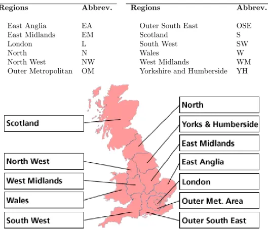
We apply the methodology described above to regional house prices (de‡ated by the general price level) in the UK using the quarterly mix-adjusted house price series collected by the Nationwide Building Society.8 The panel data set covers quarterly real house price
changes over the period 1973q4 to 2008q2 for London and11 regions.9
8The mix adjustment of the house price index is intended to correct for price variations due to location
and physical characteristics of the housing stock.
The de…nition of regions used by the Nationwide (Table 1) di¤ers in signi…cant ways from the regional de…nitions used by the O¢ ce of National Statistics which are based on the Nomenclature of Territorial Units for Statistics (NUTS) of the European Union. The main di¤erences arise with the de…nition of the North, the North West, East Anglia and the South East. The construction of the neighbourhood variables is described in Table 2. The general principle in construction was to use physically contiguous regions. However, that is not appropriate for London because the London Region is encircled …rst by the Outer Metropolitan Region which in turn is encircled by the Outer South East. In this case it may be inappropriate to rely solely on contiguity.
In general, contiguity can be a useful guide to determining the neighbours for each region. However, the relationships between house prices in di¤erent regions also interact with decisions to migrate and to commute. There are many ways in which information about house prices in di¤erent towns and regions are disseminated.10 In this regard a
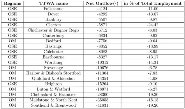
major factor in this process is migration and commuting. However, as pointed out by Cameron and Muellbauer (1998) there are many barriers to mobility, especially because of large di¤erences in the level of house prices in di¤erent regions (see also Barker, 2004). Commuting provides a substitute such that at the margin the relative price of a property of equivalent type (including an adjustment for di¤erent access to schools, countryside, etc.) at two di¤erent locations will depend on the time and cost of commuting. The extent of commuting within the UK can be seen from Table 3. This provides travel to work areas for 2001 obtained from the 2001 Census.11 In terms of net ‡ows the table reports the largest 10 areas by in‡ow and the largest 10 areas by out‡ow. London receives by far the largest in‡ow of workers each day with the large metropolitan cities of Manchester, Leeds, Glasgow and Birmingham next. In terms of out‡ows the three largest areas are Chelmsford and Braintree, Maidstone and North Kent, and Southend and Brentwood. Although some proportion of this could be to other areas, it is likely that the main destination is London. In Table 4 we identify a number of towns around London that have net out‡ows. All are connected to London via high speed rail12, and
all are in the Outer Metropolitan or Outer South East region. Of a total of 261,584 identi…ed as commuting to outside of their town some 64% of commuters come from the Outer Metropolitan Region. By contrast commuting into the other large cities is almost exclusively from within the region in which the large cities are located. So because of the connections between areas and London provided by commuting, we used the OM and OSE regions as nearest neighbours to London.13
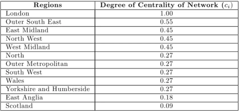
The neighbourhood connections in Table 2 with London connected to all regions forms a star network with London at its central hub. The extent of the interconnection of each region i can be measured by the degree of its centrality, ci, de…ned as the number of
regions with connections to region i divided by the total number of regions minus one.14
The degree of centrality of the regional house price network is given in Table 5. Perhaps not surprisingly Scotland turns out to have the lowest degree of centrality (0:09) with
10For example, large chains of estate agents collate information on house prices across the country and
allow the easy comparison of houses in di¤erent locations.
11These are provided by the O¢ ce of National Statistics for England and Wales and by the General
Register O¢ ce for Scotland.
12For an empirical analysis of the e¤ect on house prices of easy access to public transport (both rail
and underground) see Gibbons and Machin (2005).
13The only other region that provides a signi…cant number of commuters to London (approximately
16,000 according to the 2001 Census) is the South West. See Piggott (2007).
London (by construction) the highest. Next most connected region is Outer South East (0:55), followed by East Midland, North West, and West Midland (each with ci = 0:45).
After Scotland the least connected region turns out to be East Anglia (0:18) which is nevertheless an important commuting region to London.
An alternative measure of connection for our purposes is commuting distances of the various regions from London. This measure is particularly relevant given the central role London house prices seem to play in the process of house price di¤usion. Therefore, we consider ordering the regions (starting with London) according to their distance from London in the analysis of spatial impulse responses that follows. Regional distances from London are measured as geometrical average of distances from London to particular towns and cities in each region. For example, the distance to the North West is taken to be the geometrical average of the distance from London to Manchester, Liverpool and Lancaster.15 Note that these distances are only used in our analysis to order the
regions with respect to London. Local averages used in the regressions are measures of neighbourhood e¤ects that are de…ned in terms of contiguity and not in terms of distances.
4.2
Cointegrating Properties of UK House Prices
The logarithm of real house prices and their quarterly rates of change across the 12
regions are displayed in Figure 1. There is a clear upward trend in real house prices over the 1974-2008 period, with prices in London and Outer Metropolitan areas rising faster than other regions. The bottom panel of the graph displays the considerable variations in house price changes that have taken place, both over time and across regions. It is also interesting to note that volatility of real house price changes (around 3.5% per quarter) are surprisingly similar across all the regions except for Scotland which is much lower at around 2.7% per quarter. The average rate of price increases in Scotland has been around 0.55% per quarter which is lower than the rate of increase of real house prices in London (at around 0.76% per quarter), but is in line with the rate of price rises in many other regions in the UK with much higher price volatilities.
The time series plots in Figure 1 suggest that the price series could be cointegrated across the regions, a topic which has attracted considerable attention in the literature. See, for example, Giussani and Hadjimatheou (1991), Alexander and Barrow (1994) and Ashworth and Parker (1997). Two related issues are also discussed in the literature. One concerns the possibility that house prices are convergent across regions, namely that shocks that move regional house prices apart are temporary (Holmes and Grimes, 2008). As we shall see below this requires that house price pairs are cotrending as well as cointegrating with coe¢ cients that are equal but of opposite signs. The second issue relates to the so-called "ripple e¤ect" hypothesis, under which shocks that originate in the London area and the South East fan out across the country, with the further away regions being the last to respond to the shock (Giussani and Hadjimatheou, 1991, Peterson et al., 2002).
Cointegration of regional house prices can be tested either jointly or pairwise. A joint test would involve setting up a VAR in all of the 12 regional house price series and then testing for cointegrating across all possible regions. This approach is likely to be statistically reliable only if the number of regions under consideration is relatively small, around 4-6, and the time series data available su¢ ciently long (say 120-150 quarters).
15Because of the concentric shape of the Outer Metropolitan and Outer South East regions we used a
The pairwise approach, developed in Pesaran (2007), can be used to test for cointegration either relative to a baseline (or an average) price level or for all possible pairs of prices. When applied to all possible pairs, the test outcome gives an estimate of the proportion of price pairs for which cointegration is not rejected, as well as providing evidence on possible clustering of cointegration outcomes. This approach is reliable when N and T
are both su¢ ciently large. The full pairwise approach has been recently applied to UK house prices (over the period 1983q1-2008q4) by Abbott and de Vita (2009) who …nd no evidence of long-run convergence across regional house prices in the UK. Given the focus of our paper, namely the spatio-temporal nature of price di¤usion, the issue of whether all regional house price pairs are cointegrating is of secondary importance. Clearly, our analysis can be carried out even if none of the house price pairs are cointegrated by simply setting the error correction coe¢ cients ( is and i0) in (2.1) and (2.2) to zero for all i.
But it is important that cointegration is allowed for in cases where such evidence is found to be statistically signi…cant.
With this in mind, and given oura priori maintained hypothesis that London can be taken as the dominant region, in the left panel of Table 6 we present trace statistics for testing cointegration between London and region i house prices, computed based on a bivariate VAR(4) speci…cation in p0t and pit for i= 1;2; :::;11. The null hypothesis that
London house prices are not cointegrated with house prices in other regions is rejected at the 10% signi…cance level or less in all cases, with the exception of the Outer Metropolitan, Wales, North and Scotland. The test results for Wales and to a lesser extent for Outer Metropolitan and North are marginal. Only in the case of Scotland do we …nd no evidence of cointegration with London house prices.
Cointegration whilst necessary for longrun convergence of house prices is not su¢ -cient. We also need to establish that house prices are cotrending and that the cointegrat-ing vector correspondcointegrat-ing to(pit; p0t) is (1; 1). The joint hypothesis thatpit and p0t are
cotrending and their cointegrating vector can be represented by (1; 1) is tested using the log-likelihood ratio statistic which is asymptotically distributed as a 2
2. To carry out
these tests we use bootstrapped critical values (given at the foot of Table 6) since it is well known that the use of asymptotic critical values can lead to misleading inferences in small samples.16 The joint hypothesis under consideration is rejected at the 10% level
only in the case of Outer South East and East Anglia. Once again, these rejections are rather marginal and none are rejected at the 5% level. Together these test results support the error correction formulations (2.1) and (2.2). This does not, however, mean that all the error correction terms must be included in all the price equations. The evidence of pairwise cointegration simply suggests that one or more of the error correction coe¢ cients should be statistically signi…cant in one or both of the price equations in a given pair.
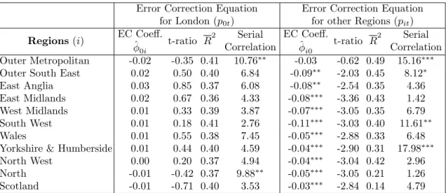
The estimates of the error correction coe¢ cients and their associated t-ratios for each price pair involving London are summarized in Table 7. The right hand panel gives the estimates for the London equation and the left panel for the other regions. As can be seen none of the error correction terms is signi…cant in the London equation, whilst they are signi…cant in the equations for all other regions, with the exception of Outer Metropolitan, which seems to have very similar features to London. These results are also compatible with London viewed as the dominant region. Prices in London are long run forcing for all other regions (with the exception of the Outer Metropolitan), whilst London is not long run forced by any other region. The concept of long-run forcing or long-run causality was …rst introduced in Granger and Lin (1995) and later applied to
cointegrating models in Pesaran, Shin and Smith (2000). It is to be distinguished from the more familiar notion of "Granger causality" which does not even allow for short term feedbacks from the non-causal to the causal regions.
4.3
Estimates of Regional House Price Equations
The regression results for a model in which London acts as the dominant region and there is the possibility of error correcting towards London and towards neighbouring regions are summarized in Table 8. Price equations for individual regions are estimated by ordinary least squares (OLS) which yield consistent estimates under the weak exogeneity of the London prices. For the London region there is no error correction term and London house price changes are regressed on their lagged values and lagged values of average house price changes in neighbouring regions. For the other 11 regions similar regressions are estimated but with contemporaneous and lagged changes in London house prices also included as additional regressors along with the error correction terms. Local averages are constructed as simple averages of house price changes of the neighbouring regions as set out in Table 2. The lag orders for each region is selected separately using the Schwarz Bayesian criterion using a maximum lag order of 4. We also used an unrestricted model of 4 lags in all variables, as well as using the Akaike criterion to select the lag orders and found very similar results.17
Estimates for the error correction coe¢ cients, i0 and is in equation (3.17), are
pro-vided in columns 2 and 3 of Table 8. The estimates, ^i0, refer to the error correction term
(pi;t 1 p0;t 1) which capture the deviations of region i house prices from London, and
^
is is associated with(pi;t 1 psi;t 1);which gives the deviations of regionith house prices
from its neighbours. In line with the literature the evidence on convergence of house prices across the regions is mixed. Considering the error correction terms measured rel-ative to London we …nd that it is statistically signi…cant in …ve regions (East Anglia, East Midlands, West Midlands, South West and North). By contrast, the error correc-tion term measured relative to neighbouring regions is statistically signi…cant only in the price equation for Scotland, with none of the error correction terms being statistically signi…cant in the remaining six regions, which include, perhaps not surprisingly, the dom-inant region, London and its surrounding regions Outer Metropolitan and Outer South East. We are left with the three regions, Wales, Yorkshire and Humberside, and North West, for which the absence of any statistically signi…cant error correcting mechanism in their price equations is di¢ cult to explain. A number of factors could be responsible for this outcome. The sample period might not be su¢ ciently informative in this regard, or these regions might have di¤erent error correcting properties that our parsimonious speci…cation can not take into account.
We now turn to the short-term dynamics and spatial e¤ects. To somewhat simplify the reporting of the estimates, in columns 4-6 of Table 8 we report the sum of the lagged coe¢ cients, with the associated t-ratios provided in brackets. Column 7 reports the con-temporaneous impact of London on other regions. The estimates show a considerable degree of heterogeneity in lag lengths and short term dynamics. Surprisingly, the own lag e¤ects are rather weak and are generally statistically insigni…cant. Own lag e¤ects are statistically signi…cant only in the regressions for the North. In contrast, the lagged price changes from neighbouring regions are generally strong and statistically highly signi…-cant, clearly showing the importance of dynamic spill-over e¤ects from the neighbouring
regions.
The contemporaneous e¤ect of London house prices are sizeable and statistically sig-ni…cant in all regions. The size of this e¤ect seems to be closely related to the commuting distance of the region from London. Wales seems to be an exception although the rather high contemporaneous e¤ects of London house price changes on Wales is partly o¤set by the large negative e¤ect of lagged London price changes. It is also noticeable that the direct e¤ect of London on the Outer South East and Wales is greater than the impact on the Outer Metropolitan Region, even though this region is physically contiguous with London.18
To ensure that the above results are not subject to simultaneity bias, we used the Wu-Hausman statistic to test the null hypothesis that changes in London house prices are exogenous to the evolution of house prices in other regions. The test statistics, reported in the 8th column of Table 8, clearly show that the null can not be rejected. This …nding is consistent with earlier evidence provided by Giussani and Hadjimatheou (1991) who use cross-correlation coe¢ cients and Granger causality tests to show the existence of a ripple e¤ect in house price changes starting in Greater London and spreading to the North. But note that there are statistically signi…cant short-run feedbacks to London house prices from its neighbouring regions. Therefore, London house prices are "Granger caused" by its neighbouring house prices, although as noted above house prices in London’s neighbouring regions are not long- run causal for London. Evidently, a dominant region could be a¤ected by its neighbours in the short-run but not in the long-run. Short-run feedbacks could be the result of forward looking behaviour on the part of the neighbours, for example.
4.4
On the Choice of the Dominant Region
Thus far we have carried out our empirical analysis on the maintained assumption that London is the dominant region. The results provided so far are in fact compatible with this view. First, we have shown in Table 7 that London prices are long-run causal for all regions with the exception of the Outer Metropolitan region. House prices in none of the other regions are long-run causal for London. Also the hypothesis that contemporaneous changes in London prices are weakly exogenous for house prices in all other regions can not be rejected (as can be seen from Wu-Hausman statistics in Table 8). We have also noted that the presence of short-term feedbacks to London from the neighbouring regions is not incompatible with our maintained hypothesis.
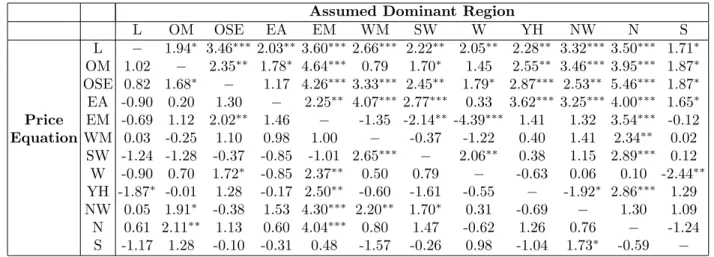
However, it is also possible that there may be other forms of pair-wise dominance. Scotland could be dominant for the North, for example. To shed light on such possibilities, in Table 9 we allow each region in turn to be ‘dominant’and then use the Wu-Hausman statistics to test the hypothesis that the assumed ‘dominant’region is weakly exogenous for the other 11 regions. The …rst column of this table con…rms the earlier results that London can be regarded as weakly exogenous for the other 11 regions. But the null hypothesis that other regions are weakly exogenous is rejected, in the case of at least 2 regions. For some regions that are relatively remote from London the number of rejections is much higher. It is also worth noting from the …rst row of Table 9 that prices changes in none of the regions can be regarded as weakly exogenous in price equation for London.
18An inspection of the ratio of London house prices to prices elsewhere suggests that since the mid
1990s house prices in the Outer Metropolitan region have declined relative to London, though a similar pattern is not apparent for other regions.
The weak exogeneity test results in Table 9 and the earlier test results of long-run causality in Table 7 provide strong evidence in favour of London being the dominant region, with the Outer metropolitan region being the second best candidate.19
4.5
A Common Factor Representation
As shown in Chudik and Pesaran (2009b) the VAR model with a dominant unit can also be viewed as a VAR with a dynamic factor. Therefore, the price di¤usion model proposed in this paper is also a dynamic factor model where the common factor is observed and identi…ed as the London price level. But in reality unobserved common factors could still be present in addition to the dominant unit(s). However, to test for such a possibility requiresN to be su¢ ciently large which is not the case in our application. An alternative speci…cation would be to assume a common factor model without a dominant unit where all regions are treated symmetrically and all price changes are related to the same unobserved common factors. Under such an approach the common factors are typically estimated as the principle components of the regional price series which again requireN to be relatively large. It is not clear to us if such a strategy would be statistically reliable in our application whereN = 12. There is also the additional di¢ culty of how to interpret the results based on common factors, since a pure common factor representation would surely destroy the spatial features that we have managed to identify and estimate within our set up.
4.6
Spatial-temporal Impulse Responses
The individual house price equations summarized in Table 8 present a rather complicated set of dynamic and interconnected relations, with the parameter estimates only providing a partial picture of the spatio-temporal nature of these relationships. For a fuller under-standing we need to trace the time pro…le of shocks both over time and across regions. Conventional impulse response analysis traces out the e¤ect of a shock over time where the time series under examination is in‡uenced by past values of itself and possibly other variables. However, when we have a spatial dimension as well, dependence extends in both directions, spatially and temporally (Whittle, 1954).
In Figure 2 we plot generalised impulse responses of the e¤ects of a positive unit shock (one standard error) to London house prices on the level of house prices in London as well as in the other 11 regions. Part A of this …gure shows the point estimates of the e¤ects of the shock on the level of house prices across all the regions, whilst part B displays the 90% bootstrapped error bounds for each region separately.
The positive shock to London house prices spills over to other regions gradually raising prices across the country. Generally the closer is the region to London the more rapid the response to the shock. Scotland in particular, but also the North and the North West take considerably longer to adjust to the shock. But the e¤ects eventually converge across all the regions, albeit rather slowly in the case of some regions. The bootstrapped error bounds also support this conclusion.
The spatio-temporal e¤ects of the London shock is better captured in Figure 3 where the same information as in Figure 2 is plotted in terms of the change rather than the level of house prices. In this …gure the responses to the London shock are plotted along the two
19The other main index of regional house prices, the Halifax, publishes a series for Greater London
dimensions with the regions ordered by distance from London. The rate of decay in the time dimension is captured by the downhill direction going from right to left. Movement initially along the ridge going from left to right captures the spatial pattern.
Another view of the results is provided in Figure 4 where the impulse response func-tions for the price changes are plotted across regions (again ordered by their distance to London) for di¤erent horizons, h = 0;1; :::12: Figure 4 is a contour of the GIRF and clearly shows the leveling o¤ of the e¤ect of the shocks over time and across regions. But the decay along the geographical dimension seems to be slower as compared to the decay along the time dimension. This important feature of the impulse response is best seen in Figure 5 where the e¤ect of a unit shock to London house prices on London over time are directly compared to the impact e¤ects of the same shock on regions ordered by their distance from London. Broken lines are bootstrap 90% con…dence band of the GIRFs for the regions. The decay of the impact e¤ects across regions is noticeably slower than the time decay of the shock on London. It is also interesting that the lower bound of the regional decay curve is systematically above the time decay curve for London, which suggests that the di¤erence in the two rates of decay could be statistically signi…cant.
4.7
E¤ects of New York House Prices
We have found that London house prices are weakly exogenous for prices in other re-gions, and long run causal. It is now interesting to ask if there are any exogenous drivers for London house price. Why should exogenous shocks to UK house prices originate in London? There are a number of possible reasons for this. London and its surrounding regions account for the largest concentration of income and wealth in the country. Macro-economic and …nancial shocks are likely to have their …rst e¤ects in London, due to the role that London has played historically as one of the world’s …nancial centres. London’s close links to New York as the pre-eminent …nancial centre in the global economy could also be an important channel through which global …nancial shocks can travel to the rest of the UK through London. With this in mind we also examined the possibility that house prices in New York have an impact on London house prices.
The NY house price series we use is based on the Bureau of Labor Statistics’de…nition of Metropolitan and non-metropolitan areas de‡ated by the New York consumer price index.20 The quarterly, time series of London and New York real house prices are shown
in Figure 6 allowing for the di¤erent scaling of the two series. There is a clear relationship between the two house price series, with London prices tending to follow New York price relatively closely. But, due to the non-stationary nature of real house price series one needs to consider such visual relationships with care.21
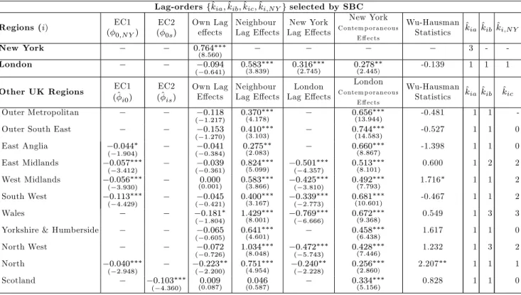
Since quarterly data on New York house price series are available only from end of 1975 onwards, we re-estimated all the regional price equations over the sample period 1976q1-2008q2 so that the estimates for the extended model are all based on the same sample information. The regression results are reported in Table 10. We …rst note that the change in the estimation sample from 1973q4-2008q2 to 1976q1-2008q2 has not a¤ected the estimates of the regional house prices and the results for these regions (reported under
20The areas included in the calculation of the NY house price series are the New York-White
Plains-Wayne Metropolitan Division comprises the counties of Bergen, NJ, Bronx, NY, Hudson, NJ, Kings, NY, New York, NY, Passaic, NJ, Putnam County, NY, Queens, NY, Richmond, NY, Rockland, NY, and Westchester, NY. For data sources and other details see Appendix A.
"Other UK Regions" in Table 10) are very similar to those reported in Tables 8.
Turning to the London price equation, we now focus on the extent to which London prices are in‡uenced by New York house prices. We …rst estimated an error correcting regression for London with the term, p0;t 1 pN Y;t 1; included as one of the regressors.
But did not …nd the error correction term to be statistically signi…cant. We then consid-ered if there were short-term feedbacks from New York to London, and run a regression of London house price changes on lagged price changes in London and New York plus the contemporaneous price change in New York. In all cases there is a statistically sig-ni…cant lagged e¤ect of New York house prices on London even when we condition on lagged neighbourhood e¤ects for London. It is also interesting that lagged e¤ects of New York house price changes on London prices are quantitatively more important than the contemporaneous e¤ect of New York house price changes on London.22
We also explored whether Paris as a major part of the market for real estate interna-tionally, might a¤ect London house prices. However, using data from 1991 on apartment prices for Paris, with the bordering departments of Hauts-de-Seine, Seine-Saint-Denis and Val-de-Marne as contiguous regions, we did not …nd any role for Paris house prices in explaining London house prices.
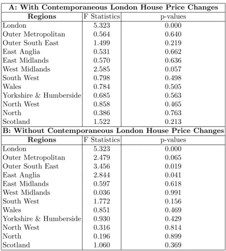
So far we have assumed that New York house price changes a¤ect UK regional house prices only through London. But it might be argued that these e¤ects could be more pervasive, possibly in‡uencing all regions directly. To test this hypothesis in Table 11 we give the F statistics for testing the joint signi…cance of the contemporaneous and lagged e¤ects of New York house prices changes in all the UK regional price equations. In panel A of the table the statistics are computed conditioning on the contemporaneous changes in London house prices, whilst in panel B only contemporaneous changes in New York house prices are included. When we condition on contemporaneous London prices the test results are highly signi…cant only in the London equation. When contemporane-ous London prices are excluded, New York hcontemporane-ouse prices become signi…cant in London’s neighbouring regions and East Anglia, but are statistically insigni…cant in other regions. These test results taken together clearly show that New York house prices are signi…cant drivers of house prices in the UK only through London.
To close the system (for the computation of impulse responses) we estimated a pure autoregression in New York house price changes. The lag order was selected by SBC which turned out to be3. The estimates are given in Table 10 and show that New York house price changes are highly persistent which is important for the way shocks transmit from New York to London and then to the rest of UK. The impulse responses of a positive unit shock to New York house prices on New York and London house price changes is given in Figure 7 and show the highly persistent e¤ects of New York house price changes on London. Initially the e¤ect of the shock is much more pronounced on New York, but after one quarter the e¤ects of the New York shock are very similar for London and New York, with the e¤ects persisting more in London than in New York, although the di¤erences are not statistically signi…cant.
For completeness, we also computed the impulse responses of the e¤ects of a unit shock to London house prices on the UK regions in the extended model with New York House prices included in the London equation. The results are summarized in Figure 8. Not surprisingly these impulse responses are very similar to those given in Figure 2 for the baseline model without New York house prices. Note that in our model a
22We also considered including changes in the GBP/US$ rate in the London house price equation, but
shock to London house prices does not feedback to New York house prices. As a result the di¤erences in impulse responses of a shock to London in the two models (with and without New York prices) are only due to the di¤erences in the parameter estimates across the two models. In the present application these di¤erences are rather small, thus explaining the similarities of the impulse responses in Figures 2 and 8.
What is of greater interest is the impulse responses of a New York shock on the level of regional house prices in the UK. The results of this shock scenario is given in Figure 9. The impact e¤ects of the New York shock on UK house prices is very small, since changes in New York house prices only a¤ect London prices directly and mainly with a lag. But once London prices start to change, as the result of the New York shock, the e¤ects begin to travel to the rest of the UK directly through the contemporaneous e¤ects of London house prices on the rest of the UK as well as indirectly through the spatial inter-linkages. The outcome is very similar to the regional impulse responses given in Table 8, with the regions further away from London being initially less a¤ected, although all regional house prices eventual convergence due to the dominant role that London plays in the di¤usion of house prices in the UK.
5
Conclusions
This paper suggests a novel way to model the spatial and temporal dispersion of shocks in non-stationary dynamic systems. Using UK regional house prices we establish that London is a dominant region in the sense of Chudik and Pesaran (2009b) and moreover that it is long run forcing in the sense of Granger and Lin (1995). House prices within each region respond directly to a shock to London and in turn the shock is ampli…ed both by the internal dynamics of each region and by interactions with contiguous regions. Using this approach we can track the di¤usion of shocks using spatial-temporal impulse responses. Furthermore, we identify an independent role for shocks to London coming from developments in house prices in New York. These proxy the e¤ect of global …nancial developments on house prices in London.
Modelling both the temporal (time series) and the spatial dimension at the same time means that we modify the conventional impulse response analysis. With a spatial dimen-sion as well, dependence is both temporal and spatial (Whittle, 1954). The results then suggest that the e¤ects of a shock decay more slowly along the geographical dimension as compared to the decay along the time dimension. When we shock London, the e¤ects on London itself die away and are largely dissipated after two years. By contrast the e¤ects of the shock to London on other regions takes much longer to dissipate, the further the region is from London. This …nding is in line with other empirical evidence on the rate of spatial as compared to temporal decay discussed in Whittle (1956), giving the examples from variations of crop yields across agricultural plots, ‡ood height and responses from population samples. A subject for further study is to see if this di¤erential pattern of decay over time and space continues to prevail in other economic applications, not only in the case of house price di¤usion, but also, for example, the di¤usion of technological innovations using a suitable economic distance.
References
[1] Abbott, A. J. and G. DeVita (2009), Testing for long-run convergence across regional house prices in the UK: A pairwise approach. Mimeo, Oxford Brookes University.
[2] Anselin, L., (1988).Spatial Econometrics: Methods and Models, Boston: Kluwer Academic Publish-ers.
[3] Alexander, C. and Barrow, M. (1994). Seasonality and co-integration of regional house prices in the UK,Urban Studies, 31, 1667-1689.
[4] Ashworth, J. and S.C. Parker (1997). Modelling regional house prices in the UK. Scottish Journal of Political Economy,44, 225-246.
[5] Bai, J., (2009). Panel data models with interactive …xed e¤ects, Econometrica, 77, 1229-1279 [6] Barker, K. (2004). Review of Housing Supply: Delivering Stability: Securing our future housing
needs. Final Report - Recommendations.www.barkerreview.org.uk. London: HM Treasury. [7] van Dijk, B., Franses, P.H., Paap, R. and van Dijk, D (2007), Modeling Regional House Prices,
Tinbergen Institute,Erasmus University, Report EI 2007-55.
[8] Bond, S.A., Dungey, M. and R. Fry (2006). A web of shocks: crises across Asian real estate markets.
Journal of Real Estate Finance and Economics,32, 253–274.
[9] Cameron, G. and J. Muellbauer, (1998). The housing market and regional commuting and migration choices.Scottish Journal of Political Economy,45, 420-446.
[10] Can, A., (1990). The measurement of neighborhood dynamics in urban house prices. Economic Geography 66, 254-272
[11] Case, B., Goetzmann, W. and K.G. Rouwenhorst, (2000). Global real estate markets: Cycles and fundamentals. NBER Working Paper No. 7566.
[12] Chudik, A. and Pesaran, M. H., (2009a). In…nite dimensional VARs and factor models,ECB working paper No. 998, January 2009.
[13] Chudik, A. and Pesaran, M. H., (2009b). Econometric analysis of high dimensional VARs featuring a dominant unit, Cambridge University, under preparation.
[14] Chudik, A., Pesaran, M.H. and E. Tosetti, (2009). Weak and strong cross section dependence and estimation of large panels, CESifo Working Paper Series No. 2689.
[15] Cli¤, A. and J.K. Ord, (1973).Spatial Autocorrelation, London: Pion.
[16] Conley, T.G., (1999), GMM Estimation with Cross Sectional Dependence,Journal of Econometrics, 92, 1-45.
[17] Conley, T.G. and G. Topa., (2002). Socio-economic Distance and Spatial Patterns in Unemployment,
Journal of Applied Econometrics, 17, 303-327.
[18] Fahrmeir, L. and C. Gössl, (2002). Semiparametric Bayesian models for human brain mapping,
Statistical Modeling, 2, 235-249.
[19] Fingleton B. (2008) Generalized Method of Moments estimator for a spatial model with Moving Average errors, with application to real estate prices,Empirical Economics, 34, 35-57.
[20] Gallin, J. (2006). The long-run relationship between house prices and income: Evidence from Local Housing Markets,Real State Economics, 34, 417–438.
[21] Garratt, A., K. Lee, M.H. Pesaran and Y. Shin, (2006). Global and National Macroeconometric Modelling: A Long Run Structural Approach, Oxford University Press, Oxford.
[22] Gibbons, S. and S. Machin, (2005). Valuing rail access using transport innovations.Journal of Urban Economics,57, 148-169.
[23] Giussani, B. and G. Hadjimatheou, (1991). Modeling regional house prices in the U.K,Journal of Financial Intermediation 13, 414-435.
[24] Gössl, C., Auer, D. P. and L. Fahrmeir, (2001). Bayesian spatiotemporal inference in functional magnetic resonance imaging.Biometrics, 57, 554-562.
[25] Goyal, S., (2007),Connections: An Introduction to the Economics of Networks, Princeton University Press.
[26] Granger, C.W.J. and Lin, J.L. (1995). Causality in the Long Run,Econometric Theory, 11, 530-536. [27] Hausman, J.A., (1978). Speci…cation tests in econometrics.Econometrica, 46, 251-272.
[28] Herring, R. and S. Wachter, (1999). Real estate booms and banking busts: An international per-spective. Wharton Working Paper Series 99-27.
[29] Holly, S., Pesaran, M.H. and T. Yamagata, (2009). A spatio-temporal model of house prices in the U.S..Journal of Econometrics,forthcoming.
[30] Holly, S. and I. Petrella, (2008). Factor demand linkages and the business cycle: interpreting aggre-gate ‡uctuations as sectoral ‡uctuations. Cambridge Working Paper No. 0827.
[31] Holmes, M.J. and Grimes A. (2008). Is there long-run convergence among regional house prices in the UK?Urban Studies, 45, 1531-1544.
[32] Horvath, M., (1998). Cyclicality and sectoral linkages: Aggregate ‡uctuations from independent sectoral shocks.Review of Economic Dynamics,1„781-808.
[33] Horvath, M., (2000). Sectoral shocks and aggregate ‡uctuations.Journal of Monetary Economics,
45, 69-106.
[34] Johansen, S., (1991). Estimation and hypothesis testing of cointegrating vectors in Gaussian vector autoregressive models.Econometrica, 59, 1551-1580.
[35] Kelejian, H.H., and Prucha, I. (1999), A generalized moments estimator for the autoregressive parameter in a spatial model,International Economic Review, 40, 509-533.
[36] Kelejian, H.H., and Prucha, I. (2009), Speci…cation and estimation of spatial autoregressive models with autoregressive and heteroskedastic disturbances,Journal of Econometrics, forthcoming. [37] Kelejian, H.H. and Robinson, D.P., (1995). Spatial autocorrelation: a suggested alternative to the
autoregressive model, In: L. Anselin and R. Florax (Eds.),New Directions in Spatial Econometrics, Berlin: Springer-Verlag.
[38] Kneib, T. and Fahrmeir, L., (2009). A space-time study on forest health. In: R. Chandler and M. Scott (eds.), Statistical Methods for Trend Detection and Analysis in the Environmental Sciences. Wiley & Sons, Hoboken, forthcoming.
[39] Lee, L.F. (2004), Asymptotic distributions of quasi-maximum likelihood estimators for spatial au-toregressive models,Econometrica, 72, 1899-1925.
[40] Pesaran, B., and Pesaran, M.H., (2009).Time Series Econometrics using Micro…t 5, Oxford Uni-versity Press, Oxford.
[41