Globalisation versus Informality: Evidence from developing countries

(1)

FIW, a collaboration of WIFO (www.wifo.ac.at), wiiw (www.wiiw.ac.at) and WSR (www.wsr.ac.at)

FIW – Working Paper

Globalisation versus Informality:

Evidence from developing countries

PHAM Thi Hong Hanh

*

A number of theoretical studies have tended to trace the nature of globalization process’ impacts (mostly characterised by trade opening) on informality, while relevant empirical literature has been not well developed. The paper aims to fill this knowledge gap by shedding further light on the linkages running from globalisation to informality in developing countries. Moreover, in this study, globalisation is characterised not only by trade integration but also by other globalisation aspects, such as social globalisation, financial globalisation and so forth. To achieve the main objective, we employ the Bayesian statistical techniques, which allow one to determine, from a large set of different globalization indicators, a subset of indicators most likely to influence the size of informality. Our finding reveals that the indicators with consistently high inclusion probabilities are trade integration, trade reforms, de jure financial openness and social globalisation. On the other hand, many covariates found significant in previous empirical studies are not robust to including in informality modelling.

JEL : F16, F41, O17, J21

Keywords: Globalisation; Informality; Bayesian Model Averaging; Developing countries

LEMNA, Institute of Economics and Management, University of Nantes Chemin de la Censive du Tertre, BP 52231, 44322 Nantes Cedex 3, FRANCE Phone: +33 (0)2 40 14 17 33, Fax: +33 (0)2 40 14 16 50

E-mail:

Abstract

The author

FIW Working Paper N° 74

October 2011

(2)

(3)

Globalisation versus Informality:

Evidence from developing countries

PHAM Thi Hong Hanh

LEMNA, Institute of Economics and Management, University of Nantes Chemin de la Censive du Tertre, BP 52231, 44322 Nantes Cedex 3, FRANCE

Phone: +33 (0)2 40 14 17 33 Fax: +33 (0)2 40 14 16 50

E-mail: [email protected]

Abstract: A number of theoretical studies have tended to trace the nature of globalisation process’ impacts (mostly characterised by trade opening) on informality, while relevant empirical literature has been not well developed. The paper aims to fill this knowledge gap by shedding further light on the linkages running from globalisation to informality in developing countries. Moreover, in this study, globalisation is characterised not only by trade integration but also by other globalisation aspects, such as social globalisation, financial globalisation and so forth. To achieve the main objective, we employ the Bayesian statistical techniques, which allow one to determine, from a large set of different globalisation indicators, a subset of indicators most likely to influence the size of informality. Our finding reveals that the indicators with consistently high inclusion probabilities are trade integration, trade reforms, de jure financial openness and social globalisation. On the other hand, many covariates found significant in previous empirical studies are not robust to including in informality modelling.

Keywords: Globalisation; Informality; Bayesian Model Averaging; Developing countries

(4)

1. Introduction

Over the last decade, globalisation has become a phenomenal aspect of the world economy. In terms of trade globalisation, by 2008, the ratio of trade flows to the world GDP valued at around 60%, compared with less than 40% in the mid-1990s. Similarly, in terms of cross-border financial transactions, FDI net flows reached more than 6% of the world GDP, while this figure only attained to less than 2.5% in the mid-1990s.1_{By and large, globalisation}

process is believed to strongly affect the world economic growth as well as other macroeconomic aspects. Among others, this paper pays a special attention to possible causal linkages running from globalisation to informality in developing countries.

In the literature, the existing theoretical works have seemed to only focus on possible effects of “trade globalisation” aspect on informality. Concerning this issue, existing theoretical studies can be classified into two groups. Firstly, basing on the Harris-Todaro (1970) dual-economy model of rural-urban migration, Chandra and Khan (1993) and Marjit and Beladi (2007a) suggest that tariffs reduction results in a raise in both employment and wages in the informal sector when informal output is traded. By contrast, according to Beladi and Yabuuchi (2001), trade opening may decrease the size of informal employment when informal outputs are used as intermediate inputs in the formal sector. Secondly, in the light of trade models with differentiated wages, when capital is sufficiently mobile, trade integration can boost both informal employment and informal wages (Marjit and Maiti, 2005; Kar et al., 2003). In order to validate different theoretical hypotheses, empirical works have been developed and mostly available for a small group of Latin American countries. According to these studies, impacts of trade opening on informal economy strongly depend on country-specific circumstances. For instance, trade integration reduces informal activities in Mexico (Maloney, 1998), but increases informality size in Colombia and has no significant impact on Brazilian informal employment (Goldberg and Pavcnik, 2003b).

While globalisation process is manifold dimensions: economic (including trade and financial), social, political, cultural, environmental and so forth, the previous cited studies have only deepened our understanding of trade opening’s impacts on informality. They have seemed to ignore impacts of other important globalisation aspects. Recently, using a new database of International Labour Organisation (ILO), Bacchetta et al. (2009) tend to clarify the multi-dimension of globalisation process as well as to investigate its impacts on informal

1_{Author’s computation from WDI data}

(5)

employment of developing countries. In order to capture the multifaceted nature of globalisation, the authors introduce in their estimated models a large set of globalisation indicators drawn from various international sources. The authors draw a mixed picture of globalisation’s impacts on informal employment in developing countries. On one hand, they suggest that more open economies may have a lower incidence of informal employment. On the other hand, trade reforms seem to associate with higher informal employment. Similarly, larger FDI inflows may lead to an increase in informal employment. Complementing to the work of Bacchetta et al. (2009), Fugazza and Fiess (2010) use three different data sets to assess the sign of such a complex relationship. This work also draws a mixed picture and no clear-cut conclusion regarding the connection between globalisation and informal employment. In a cointegration framework, more openness to trade is associated with greater informal employment and output for most countries, while lower trade restrictions appear to generate lower informal employment and output in most cases. However, the system-GMM estimation generates contrasting results that fewer trade restrictions associate with more informal output but less informal employment. Up to now, the works developed by Bacchetta et al. (2009) and Fugazza and Fiess (2010) can be seen as the pioneer ones that endeavour to trace possible impacts of all globalisation dimensions on informal employment of developing countries. These works have focused on regression models involving a large and specific set of covariates collected from various data sources and regrouping information on different aspects of globalisation. Nevertheless, this empirical strategy seems to ignore uncertainty regarding the model specification itself, which can have dramatic consequences on inference, because the inference regarding the effects of included covariates can depend critically on the inclusion versus the exclusion of other covariates. Consequently, the potential uncertainty problem may lead to little agreement on the relationship between globalisation and informality between these two recent empirical studies.

So that, in our present paper, we aim to revisit potential affects of different globalisation dimensions on informality in developing countries by employing another empirical technique that is the Bayesian Model Averaging (BMA) technique. Employing the BMA technique allows us to confront uncertainty regarding the appropriate set of covariates to include in a regression model explaining informality. Moreover, differing from earlier empirical works, which aim to clarify the nature (positive or negative, significant or insignificant) of globalisation’s impacts on informal employment, the main objective of this paper is to

(6)

determine, from a large set of potential covariates, a subset of globalisation indicators with high inclusion probabilities in the “true” informality model.

The reminder of this paper is organised as follows. Instead of providing a brief literature review of globalisation’s impacts on informality that has been extensively documented in the orthodox work of Bacchetta et al. (2009), Section 2 outlines our empirical strategy that encompasses specifying the BMA technique. Section 3 describes different datasets being used for the testing. Section 4 reports and analyses the econometric results as well as robustness checks, and makes comparisons to related literature. Concluding remarks are in

Section 5.

2. Empirical model specifications

As mentioned, to achieve the research objective, we employ here the BMA technique for which the statistical foundation is extensively documented in excellent surveys by Raftery (1995) and Hoeting et al. (1999). In the empirical literature, the BMA technique has been widely accepted as a way of accounting for model uncertainty, particularly in regression models for identifying the determinants of economic growth (e.g. Leamer, 1978; Levine and Renelt, 1992; Fernandez et al., 2001a, b; Sala-i-Martin et al., 2004). Moreover, BMA has been also used to evaluate an extensive set of potential determinants of other macroeconomic variables, notably FDI determinants (e.g. Eicher et al., 2011; Blonigen and Piger, 2011). Hence, in this paper, applying the BMA technique allows us to identify globalisation indicators, which truly affect informality in developing countries, from a large set of potential indicators.

Specifically, we focus on the following linear regression model:

(

I

)

N with X y i i i 2 , 0

σ

ε

β

α

+ + ≈ = (1)

where y is the dependent variable holding the size of informality,

α

_iis a constant, X_iis a set of potential independent variables explaining the dependent variable y,

β

_iis the coefficients, and

ε

is a normal independent and distributed (IDD) error term with mean zero and variance

σ

2

. If there are many potential explanatory variables in a matrix X, we are interested in two questions: Which appropriate variables X_i∈

{ }

X should be included in the model? And how important are they? However, the fact is that the direct approach to do inference on a single linear model with all potential explanatory variables X is inefficient or even infeasible with a limited number of observations.

(7)

Now, suppose X contains K potential variables and the model uncertainty problem in (1) is mainly due to the selection of variableX_i. In this case, a particular selection of X_idefines the

th

i model, denotedM_i. If the variable Xi∈

{ }

X can be freely included in the regression model, there are K

2 variable combinations and thus K

2 models to consider. The Bayesian approach tackles the uncertainty problem by estimating alternative models for all possible combinations of

{ }

X

and constructing a weighted average over all of them. In the Bayesian words, the posterior probability that M_iis the “true” model of y is as follow:

(

)

(

_{( )}

) ( )

(

₍

) ( )

_{) ( )}

∑

₌ = = K j j j i i i i i M p X M y p M p X M y p X y p M p X M y p X y M p ₂ 1 , , , , (2)

where p

( )

M_i is the prior probability that M_iis the "true" model,

p

( )

y

X

denotes the marginal or integrated likelihood which is constant over all models and is thus simply a multiplicative term. Therefore, the posterior model probability (PMP)

p

(

M

_i

y

,

X

)

is proportional to the marginal likelihood of the model

p

(

y

M

_i

,

X

)

.

Turning now to our regression model, the PMP can be used to confront the model uncertainty present in the informality regression. The PMP allows us to select the “true” model with highest posterior probability and then to make inference about other alternative models based on this “best” model. Nevertheless, if the PMP is widely dispersed across a large number of models, making inferences from a single and highest probability model can yield biased empirical results. Hence, instead of the PMP, the BMA technique calculates the averaging posterior inference across all alternative models. Precisely, for any statistic

θ

, the BMA posterior distribution is calculated as:

(

y X

)

p

(

M y X

) (

p M X y

)

p _i i i K , , , , 2 1

∑

₌ =

θ

(3)

where

p

(

θ

M

i

,

y

,

X

)

represents the posterior distribution for

θ

conditional onMi. The BMA

posterior distribution

p

(

θ

y

,

X

)

is not conditioned on a particular model, which is the “true” model, but is conditioned on the data. Hence, BMA is believed to confront uncertainty regarding the appropriate set of covariates included in a regression model.

In order to implement BMA, specifications for both the prior model probability p

( )

M_i and the prior density function for the parameters

{

α

,

β

,

σ

}

of M_i are required. Suppose the prior

(8)

model probability is p

( )

M_i uniform with respect to all alternative models, it is calculated as follow:

( )

Mi K p 2 1 = (4)

The prior model probability specification (4) is a common choice in BMA approaches. It means that the prior probability of any single covariate in the “true” model is at least 50%. Unlike the specification of prior model probabilityp

( )

M_i , that of prior parameter densities is not an easy task.

In our analysis, we use two different automatic procedures for setting parameter priors. First, we take into consideration a Bayesian regression linear model with a specific prior structure called “Zellner's g prior”. Following this procedure, each individual model M_iis considered as a normal error structure. In order to specify the priors on the model parameters, we assume that constant

α

_iand error term

ε

have improper priors, meaning they are evenly distributed. Hence, the implementation of BMA only depends on the specification of curial prior probability of coefficients

β

_i. Here, we formulate the prior beliefs on coefficients into a normal distribution with a specified mean and variance. According to Zellner's g setting, the variance

structure is defined as follow:

1 ' 2 1 −       i iX X g

σ

with

























≈

−1 ' 2

1 ,

0

_i _i i

X

g

N

g

σ

β

The previous formula means that the coefficients

β

_iare believed to be zero and that their variance-covariance structure is in line with that of X. The parameter g embodies how certain one is that the coefficients

β

_iare zero. A small g corresponding to few prior coefficient variance implies one is quite certain that the coefficients are indeed zero. By contrast, a large

g means that one is very uncertain that the coefficients are zero. Hence, the specification of prior of coefficients

β

_iconcerns the value of the parameter g. In the literature, g value is set through a popular default approach so-called the Unit Information Prior (UIP), which sets

N

g= commonly for all modelsM_i. According to Kass and Wasserman (1995) and Rafery (1995), the UIP setting suggests a convenient approximation to the marginal likelihood based on the Bayesian Information Criterion (BIC). For this reason, the UIP procedure seems to be simple to implement.

(9)

In the second step, as a robustness check, we employ an alternative prior specification developed by Fernandez et al. (2001a) (henceforth, the FLS). Unlike the UIP procedure, the FLS setting should be applied if one wishes to use little subjective information in setting prior densities. In addition, Fernandez et al. (2001a) employ a uniform model prior and the birth-death Markoz Chain Monte Carlo (MCMC) sampler.2_{Differing from the UIP approach}

withg =N , in the FLS procedure g prior is set to

(

2

)

; max N K

g = .3

3. Data issues

Our empirical study is based on an unbalanced annual panel data covering various individual indicators, such as the size of informality, globalisation indicators and other macroeconomic indicators, for a selected sample of developing countries over the period 1990-2006 (see ANNEX 1 for a detailed description of the data and their sources).

Informality data

The data sets covering the size of informality in developing countries come from two principal sources. The first data set used in this paper is available in the ILO’s Key Indicators of the Labour Market (KILM) database. As defined in the ILO report (1993) on “Decent Work and the Informal Economy”, informal employment of a country comprises:

own-account workers and employers who have their own informal sector enterprises;

contributing family workers, irrespective of whether they work in formal or informal sector enterprises;

employees who have informal jobs, whether employed by formal sector enterprises, informal sector enterprises, or as paid domestic workers by households;

members of informal producers’ cooperatives;

persons engaged in the own-account production of goods for own final use by their household (e.g. subsistence farming, do-it-yourself construction of own dwellings). The ILO informal employment database allows us to construct an unbalanced panel for 49 countries (17 Latin American countries; 11 Asian countries; 15 African countries; and 6 East and Central European countries) over the period 1990-2006. Here the size of informality is measured by the ratio of informal employment to total employment.

2_{“Birth-death MCMC sampler is the standard model sampler used in most BMA routines. One of the K potential}

covariates is randomly chosen; if the chosen covariate forms already part of the current model Mi, then the

candidate model Mj will have the same set of covariates as Mi but for the chosen variable. If the chosen covariate

is not contained in Mi, then the candidate model will contain all the variables from Mi plus the chosen covariate”

(Zeugner, 2011).

(10)

The second data set used in this paper employs the shadow economy estimates of informal activity developed by Schneider (2005, 2007), which are derived from a combination of the Currency Demand Approach and the dynamic multiple-indicators multiple causes (DYMIMIC). Schneider (2005) provides a snapshot of informality for 110 countries in 1990/91, 1994/95 and 1999/2000, and then Schneider (2007) provides annual observations for the same countries over the period 2000-2004. However, in order to consist with the country sample in the first data set, we only use the shadow economy estimates by Schneider for 49 developing countries of interest. In this second data set, the size of informality is measured as the share of informal sector’s GDP in official GDP.

Globalisation indicators

As mentioned, globalisation is manifold dimensions. In this paper, we pay our attention to two main dimensions of globalisation process, notably economic and non-economic dimensions. In order to capture the non-economic dimensions of globalisation, we use a number of different globalisation indicators developed by the Zurich-based Konjunkturforschungsstelle (KOF) (Dreher et al., 2008), including three social globalization indicators and one political globalization indicator (see Annex 2). Likewise, we classify economic dimension of globalization process into three sub-dimensions:

First, to measure general degree of economic globalization of a given country we use the “Actual economic flows” indicator also provided by Dreher et al. (2008). This indicator presents a weighted average of trade, foreign direct investment, portfolio investment and income payments to foreign nationals.

Second, the financial dimension of globalization is measured through two alternative indicators being considered as “de facto” one or “de jure” one. The “de facto” indicator is calculated as the ratio of foreign assets and liabilities to GDP.4_According

to Baltagi et al. (2009), the advantage of this indicator is to provide a useful summary of the financial integration progress of a country. We also deploy the second “de facto” indicator, which is considered as the share of FDI inflows in GDP. Whereas the “de jure” indicator is the Chinn and Ito (2006) index of capital account openness (KAOPEN)5_{that is widely used in previous cross-country studies.}

Third, to capture trade globalisation dimension we use a broad set of indicators. The first one is the trade openness indicator. Among others, the most well-known trade

4_{This indicator is initially constructed by Lane and Milesi-Ferretti (2006).} 5_{Available at:}_{http://www.ssc.wisc.edu/~mchinn/research.html}_.

(11)

openness indicator is the Sachs and Warner (1995) index.6_{Although this index serves as}

a proxy for a wide range of policy and institutional differences and not only of trade policy (Rodriguez and Rodrik, 1999), it can only suggest that a country is either open or closed. Also, this index is difficultly constructed due to the unavailability of many data components. Furthermore, the statistical correlation between the SW index and other variables of interest is not always obvious and difficult to set an econometric model and to interpret the empirical results. For these reasons, we deploy a standard trade openness indicator measuring the sum of exports and imports to GDP. The second one is a set of de jure trade openness indicators including: i) Trade restrictions; ii) Most-favoured nation (MFN) rate; iii) Revenue from trade taxes. The last one comprises the diversification and concentration index of exports and imports.

Data setting

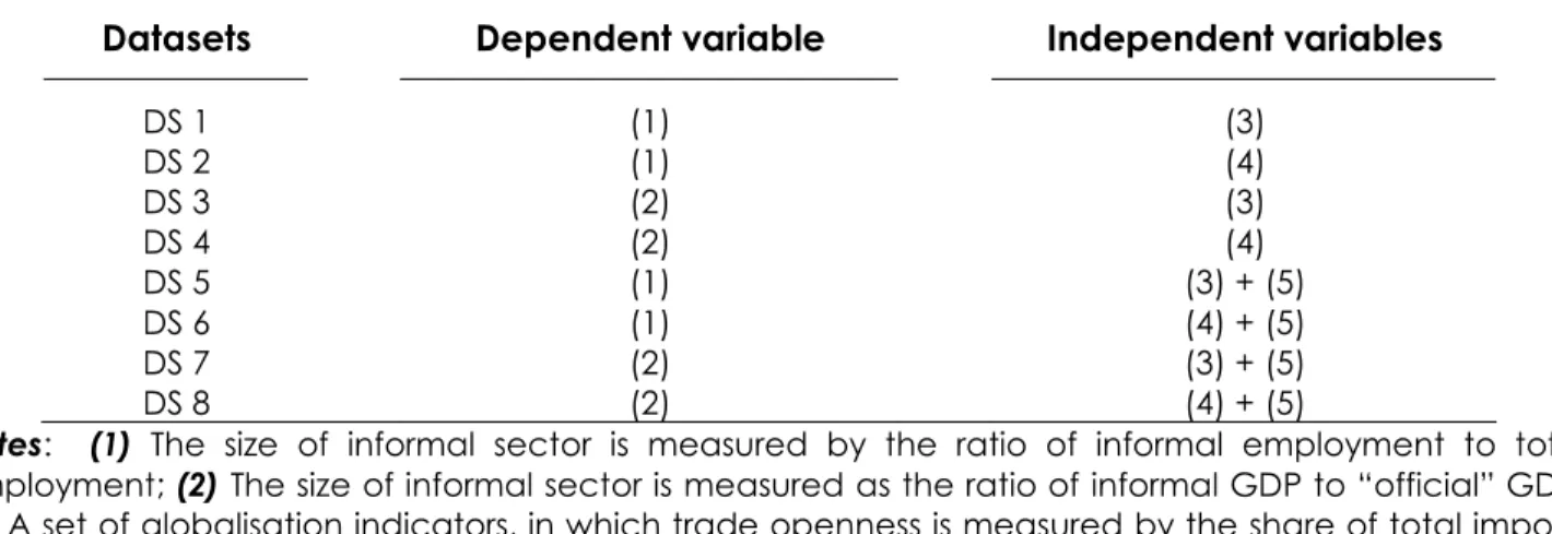
Remind that the main objective of this paper is not to identify the determinants of informal employment in developing countries, but is to clarify the multi-dimensions of globalisation process and their possible impacts on informality of developing countries by employing the BMA technique. Thus, the inclusion of other explanatory variables beside a large number of globalisation indicators is not strongly required. However, in order to compare our BMA results to those of previous studies (Bacchetta et al., 2009; Fugazza and Fiess, 2010), together with a data set only including globalisation indicators, we build another dataset that includes both globalisation indicators and other macroeconomic indicators collected from various international sources. The choice of these additional explanatory variables is strongly based on Bacchetta et al. (2009) and Fugazza and Fiess (2010) (see further Annex 2). Besides, to gain a better understanding of impacts of trade integration on informal employment, we construct another alternative dataset, in which we use two separate trade openness indicators, notably exports to GDP ratio and imports to GDP ration, instead of the ratio of total exports and imports to GDP. By and large, our empirical study is based on eight alternative data sets summarised in Table 1.

6_{The SW index, which is constructed by Sachs and Warner (1995), is a dummy variable for openness based on five}

individual dummies for specific trade-related policies. Relying on this index, a country is classified as closed if it displays at least one of the following characteristics: Average tariff rates of 40 percent or more; Non-tariff barriers covering 40 percent or more of trade; A black market exchange rate that is depreciated by 20 percent or more relative to the official exchange rate, on average, during the 1970s or 1980s; A state monopoly on major exports; A socialist economic system.

(12)

Table 1: Data setting’s outline

Datasets Dependent variable Independent variables

DS 1 (1) (3) DS 2 (1) (4) DS 3 (2) (3) DS 4 (2) (4) DS 5 (1) (3) + (5) DS 6 (1) (4) + (5) DS 7 (2) (3) + (5) DS 8 (2) (4) + (5)

Notes: (1) The size of informal sector is measured by the ratio of informal employment to total employment; (2) The size of informal sector is measured as the ratio of informal GDP to “official” GDP;

(3) A set of globalisation indicators, in which trade openness is measured by the share of total imports and exports to GDP; (4) A set of globalisation indicators, in which trade openness is measured by exports/GDP ratio and imports/GDP ratio; (5) A set of other explanatory variables;

4. Empirical analysis

This section reports and discusses the BMA results. It also reports the results of an alternative econometrical technique that check the sensitivity of the results to different estimation methods and different data settings. Finally, we compare our main findings with those of related literature.

Estimation results

The main results are presented in Tables 2-5. Tables 2 and 3 contain the BMA estimates of restrictive regressions that only include various globalisation indicators in the matrixX_i. Tables 4 and 5 report the BMA estimates of a larger regression comprising both globalisation indicators and other macroeconomic indicators. In addition, Tables a present the results using the data set with the sum of exports and imports to GDP as a de facto trade openness indicator, while Tables b report the results using the dataset with two separate ratios, exports/GDP and imports/GDP. In all reporting tables, the importance of the covariates in explaining the dependent variables is given in the first column PIP, which represents posterior inclusion probabilities calculated through the UIP procedure. The second column displays the coefficients averaged over all models, including the models wherein the variable was not contained (implying that the coefficient is zero in this case). The last column presents the robustness test from the FLS alternative prior specification.

Results for the ILO datasets

We begin with the empirical results using the ILO datasets (reported in Tables 2 and 4), in which the size of informal sector is measure as the ratio of informal employment to total

(13)

employment. Going straight to question of interest, we note that among 14 different globalization indicators, only 3 variables have inclusion probabilities above 50% in the levels specification, meaning a fairly parsimonious globalization dimensions are sufficient to explain the size of informal sector in developing countries. Globalization indicators have high inclusion probabilities are trade openness, KAOPEN index and personal contacts level. On the other hand, our empirical results show that broad categories of globalization dimensions have received little statistical support, particularly those related to the MFN rate, actual economic flows and foreign assets and liabilities. From these results, many comments may arise.

Firstly, trade openness measured as the share of total trade in GDP plays a significant role in explaining informal employment. We see that with 99.7%, virtually all of posterior informality model include trade openness indicator. Moreover, its unconditional coefficient is positive, meaning that more openness to trade generates larger size of informal employment. However, this coefficient is quite low (0.13). This suggests that trade openness plays a significant but not much important role in increasing the size of informal employment. In the case of separately using exports/GDP ratio and imports/GDP ratio as two de facto trade openness indicators, we find that the inclusion probability of imports is high (97.9%) while that of exports is fairly small (only 7.9%). This result indicates different impacts of imports and exports on informal employment: imports growth seems to be correlated with more informality while exports growth is not sufficient to explain informal employment rates. Unlike a high inclusion probability of de facto trade openness, all other trade indicators have such a small PIP value. It means that trade reforms in developing countries plays an insignificant role in explaining the evolution of their informal labour markets. In other words, even though trade reforms require an economic adjustment process and labour reallocation across sectors in developing countries, such reforms may only have impacts (positive or negative) on formal sector.

Secondly, we also obtain mixed results regarding the impacts of financial globalization on informal employment. With a high inclusion probability (58.7% and 59.5%), KAOPEN index, a

de jure financial openness indicator, confirms its significant role in explaining the size of informal employment. Precisely, less restrictions on cross-border financial transactions lead to higher informal employment rates. Conversely, with small PIP values, both inward FDI flows and foreign assets seem to have no impact on informal employment. This result could be interpreted as evidence that most foreign investment inflows take place in the formal sector.

(14)

However, if we take into consideration the structuralism hypothesis of the informal economy serving the formal sector, foreign investment could still increase informality rates through an indirect channel: foreign investment inflows encourage the development of formal sector, which in turn lead to an enlargement of informal sector to respond to larger demand of formal sector. This hypothesis will be considered in our further research.

Looking now at non-economic dimensions of globalization, our empirical results also offer a mixed picture. On one hand, the covariate “personal contacts” has a most important PIP value (100%) and a negative coefficient. Accordingly, personal contacts level has helped to reduce informality in our sample developing countries. On the other hand, with small PIP values, other social and political globalization indicators do not seem to matter much. Consequently, their coefficients are quite low.

We now turn our attention to Tables 4a and 4b, in which the BMA estimates are reported for a larger dataset including both globalization covariates and other ones. Despite the different magnitudes of each PIP and PM value, the qualitative nature of our results regarding all globalisation covariates, by and large, remains unaltered in this dataset. Furthermore, we also find another set of 6 variables out of the 13 additional potential covariates that have high inclusion probabilities (above 50%). These 6 variables can be classified into two sub-categories: the size of economy (GDP and population indicators) and regulation (government spending, rule of law and government accountability). In terms of economic size, a high PIP value and a negative coefficient of GDP per capita indicates that an increase in economic development level can reduce informal employment in developing countries. In addition, population-related indicators, which have been used to control for the growth of labour force, have also a remarkable impact on informal employment. Regarding the regulatory environment, our empirical results nevertheless provide a more nuanced picture of the connection between government regulation and informal employment. With a high PIP and a negative coefficient, governance efficiency can be shown to contribute to a decline in informal rates. By contrast, regarding to the rule of law, we obtain such a “curious” result. A negative coefficient of this covariate implies that high informality rates seem to be an undesired outcome of the rule of law in our sample developing countries. Likewise, labour market regulation measured as decentralised wage bargaining systems and minimum wage levels has no effect on informal employment. It embodies that the adjustments in labour

(15)

market regulation have been not enough efficient to allow developing countries to increase formalisation rates and to decrease the size of informal sector.

Results for Schneider’s shadow economy datasets

Now we look at the empirical results (reported in Tables 3 and 5) for Schneider’s shadow economy datasets, in which the share of informal GDP in “official” GDP is used as a measure of the average size of shadow economy. Above all, using Schneider datasets our results provide only partial support to previous results using the ILO datasets, which stipulates that economic integration, here characterized by the KAOPEN and trade openness covariates, plays an important role in explaining the growth of shadow economy. In detail, posterior inclusion probabilities of KAOPEN index, trade openness indicator and imports ratio have a high value of 97.7%, 99.8% and 100% respectively. This is also true if economic integration is replaced by a more general concept “Actual economic flows” that represents a weighted average of trade, FDI, portfolio investment and income payments to foreign nationals. Moreover, the negative value of exports coefficient (-0.28 in Table 3b) indicates that exports growth can be shown to contribute to high formalization rates that in turn reduce shadow activities. Together with these similar results, we find a broad set of different results as using the shadow economy dataset.

Firstly, we obtain PIP value above 50% for two trade reforms indicators, notably trade restrictions and MFN rate. In addition, the coefficients of these covariates are negative, meaning that trade reforms seem to be correlated with less informality. At the same time, the relative concentration and diversification of merchandise exports have high PIP values. Moreover, these two covariates have a comparatively large coefficient and seem to be most important. However, they have quite different impacts on shadow economy. While trade concentration may reduce shadow activities, trade diversification may lead to the deepening of informal sector. Regarding other globalization indicators, the empirical results confirm the role of cultural proximity in reducing informality in developing countries.

Examining now the results relating to a larger shadow economy dataset in Tables 5a and 5b, we first note that the effects of economy size (characterized by GDP per capita and population-related indicators) appear to be either quantitatively or qualitatively similar to those obtained for the ILO dataset. Specifically, higher level of GDP per capita can lead to less informality while the population growth has been considered as a main source of informality in developing countries. Tables 5a and 5b also list other explanatory variables that

(16)

have high inclusion probabilities, including top marginal tax rates, transfers and subsidies, and corruption. Among others, high marginal tax rates for top earners seem to foster shadow economy. This result is in line with those presented in the literature assuming that high marginal tax rates would set incentives for high-skilled employees to become informal. Also, transfers and subsidies tend to contribute to the enlargement of shadow economy. By contrast, a negative coefficient of corruption index embodies that the growth of shadow economy probably results from a high level of corruption.

By and large, regarding a group of covariates including de facto trade openness, de jure

financial openness, economy size-related indicators and government effectiveness, our empirical analysis gives similar findings from both ILO and Schneider datasets. Relating to other globalization indicators and a set of additional macroeconomic variables, our findings are different across these two datasets. Table 6 provides a comparison of main findings.

Our different empirical results are probably due to the differences in data setting. First, the ILO dataset is an unbalance panel data, which covers information on informal employment of 55 developing countries over the period 1990-2006. By contrast, the Schneider dataset is a balance panel data, which provides information on economic growth of shadow economy during three shorter periods 1990/91, 1994/95 and 1999-2004. Second, each dataset is based on a given definition of concept “informality” as well as a given method of estimating informality rates. The ILO database defines “the informal sector as production units operated by single individuals or households that are not constituted as separate legal entities independent of their owners and in which capital accumulation and productivity are low”, while Schneider (2005) defines “the shadow economy includes all market-based legal production of goods and services that are deliberately concealed from public authorities for the following reasons: (1) to avoid payment of income, value added or other taxes, (2) to avoid payment of social security contributions, (3) to avoid having to meet certain legal labor market standards, such as minimum wages, maximum working hours, safety standards, etc., and (4) to avoid complying with certain administrative procedures, such as completing statistical questionnaires or other administrative forms”. Likewise, to estimate the size of informality, the ILO dataset employs the direct methods7_{while Schneider (2005, 2007) applies}

7_{The direct methods are microeconomic in nature and use either voluntary survey data or the results from tax}

audits to construct estimates of total economic activity and its official and unofficial (or measured and unmeasured) components.

(17)

an indirect and modeling approach, which is a comparison of the DYMIMIC model and currency-demand model.

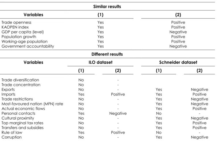
Table 6: Main findings Similar results

Variables (1) (2)

Trade openness Yes Positive KAOPEN index Yes Positive GDP per capita (level) Yes Negative Population growth Yes Positive Working-age population Yes Positive Government accountability Yes Negative

Different results

ILO dataset Schneider dataset

Variables

(1) (2) (1) (2)

Trade diversification No - Trade concentration No -

Exports No - Yes Negative Imports Yes Positive Yes Positive Trade restrictions No - Yes Negative Most-favoured nation (MFN) rate No - Yes Negative Actual economic flows No - Yes Positive Personal contacts Yes Negative No - Cultural proximity No - Yes Negative Top marginal tax rates No - Yes Positive Transfers and subsidies No - Yes Positive Rule of law Yes Positive No - Corruption No - Yes Negative

Variables with low inclusion probabilities in both datasets: Most-favoured nation (MFN) rate; Trade restrictions; Revenue from trade taxes; FDI; Foreign assets and liabilities; Information flows; Political globalization; GDP growth; Government spending; Price controls; Minimum wages; and Wage bargaining.

Notes: (1) High inclusion probabilities; (2) Nature of connection with informality

Even though we find a broad set of different results from two datasets, these results are not contrary each other. Importantly, the results from Schneider’s dataset seem to complement to those obtained from the ILO dataset, and vice versa.

Robustness checks

As revealed, the BMA estimates suggested by Fernandez et al. (2001a) are carried out to examine the sensitivity of our empirical results to alternative estimation strategies and datasets. Here we only report the PIP values estimated by the FLS method in the last column of Tables 2-5. Even though the magnitudes of each estimated PIP are different compared to those obtained from the IUP approach, the qualitative nature of our results remains unaltered

(18)

across different datasets. It supports that our empirical results are robust to a range of alternative measures, datasets and estimation approaches.

Comparisons with earlier studies

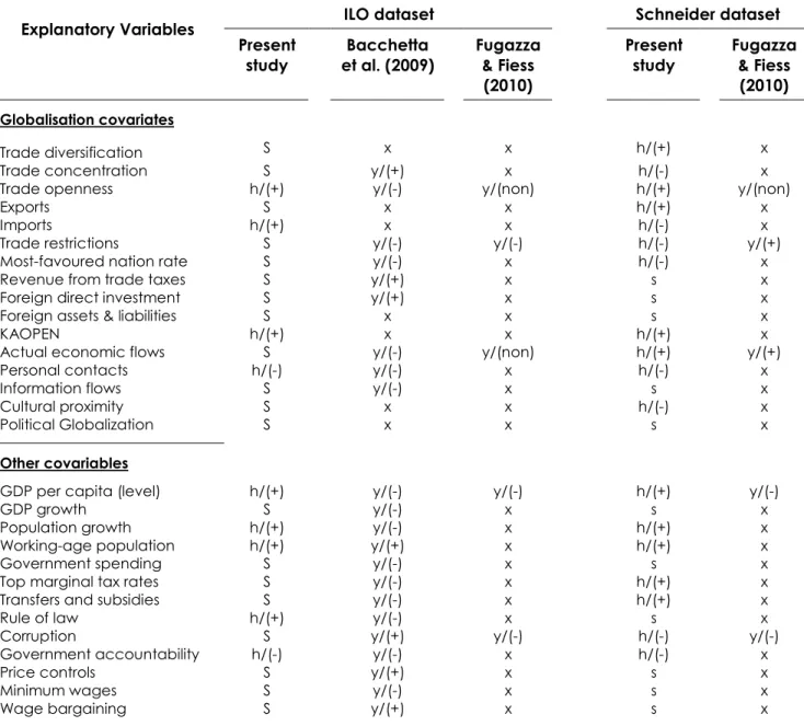
With the BMA results in hand, we now turn to address another question of how these results compare to those of previous studies. Reminder that empirically investigating the relationship between globalisation and informality for a large sample of developing countries has not received the attention. Up to now, there have been only two recent empirical works that tend to develop this issue, one by Bacchetta et al. (2009) and another by Fugazza and Fiess (2010). Our results, particularly those related to the ILO dataset can be compared with those of Bacchetta et al. (2009) who also use the same dataset. On the other hand, our results, which are obtained from Schneider’s dataset, can be compared with those suggested by Fugazza and Fiess (2010). We list our main findings as well as those of two cited previous studies in Table 7.

The work developed by Bacchetta et al. (2009) aims to clarify such a complex interaction between globalisation and informal economy in developing countries. To do so, their empirical analysis is based on the ILO database providing information on informal employment for 31 developing countries. In addition, the multifaceted nature of globalisation process is measured not only by trade integration indicators but also by financial, social and political globalisation indicators. The authors also include in their estimation models a large number of other macroeconomic variables. In general, our present study uses the same indicators favoured in Bacchetta et al. (2009). However, our findings provide only partial support to those of Bacchetta et al. (2009). Specifically, our findings are consistent with those suggested by Bacchetta et al. (2009) on role of various variables (e.g. personal contacts, GDP per capita, working-age population, and government effectiveness) in explaining the size of informal employment in developing countries. Regarding trade openness, according to Bacchetta et al., this globalisation dimension seems to be correlated with less informality. In sharp contrast, we find that trade openness, particularly imports growth, can increase informality rates in developing countries. Here, our finding seems to be consistent with much of theoretical models supporting a positive connection between trade opening and informality. Also, differing from Bacchetta et al., who exclude de jure financial indicator in their regression estimations, our empirical results indicate that this indicator (KAOPEN index) having a high PIP and a positive coefficient can be shown to contribute to an increase in

(19)

informality rates. In other words, capital account openness or global capital mobility has become a determinant factor of the deepening of informal activities in developing countries. This finding seems to complement to the theoretical hypothesis of Marjit and Acharyya (2003), who argue that the impact of globalisation on informality depends on the degree of capital mobility between the formal and the informal economy. Looking at other covariates (e.g. trade reforms, political globalisation, government policies and regulation), Bacchettat et al. (2009) find that all these variables enter significantly in all estimations and consequently have positive or negative impact on informal employment. Yet, employing the BMA technique, we obtain a fairly small PIP value for each of these variables. It means that they should not be considered as appropriate covariates to include in a regression model explaining informal employment in developing countries.

In another related empirical work, Fugazza and Fiess (2010) only tend to assess the sigh of the relationship between trade liberalisation and informality. In their study, three different datasets are used: ILO micro-founded data; ILO survey-based data; and Schneider estimates. Here, we only refer to the findings of Fugazza and Fiess (2010) that are obtained from two latter datasets. Also, it should be worth noting that in Fugazza and Fiess (2010) all datasets include information on informal sector for both developed and developing country. Additionally, with respect to their research objective, the authors only include a narrow set of trade globalisation indicators in their regression estimation, notably de facto trade openness indicator (trade/GDP) and trade restrictions. Above all, employing the generalised method of moments (GMM) of Arellano and Bond (1991) as well as the system-GMM of Blundell and Bond (1998), Fugazza and Fiess fail to identify the nature of the relationship between de facto

trade liberalisation and informality in all estimations. Besides, using the same Schneider dataset, while our empirical results signify that informal output falls with more restricted trade, Fugazza and Fiess find contrasting evidence that more trade restrictions is always associated with a larger share of informal output in total GDP. Nevertheless, relating to variable “actual economic flows”, our empirical study offers a similar finding with that of Fugazza and Fiess. Specifically, higher economic flows generate higher share of informal output, while this variable has no significant impact on informal employment.

To this end, the differences in empirical findings between our study and the two previous works may be explained by the fact that the model specifications are not identical, the estimation procedures are not the same and the data setting and frequencies used for

(20)

estimation are different in each study. Furthermore, there is also little agreement on the nature of such a complex relationship between globalisation and informality in earlier theoretical studies. Therefore, little empirical consensus on this relationship has been ineluctable. Notwithstanding these important differences, it is always useful to carry out such a comparison that allows us to clarify the extent of our current contribution in the context of related literature.

5. Concluding remarks

This paper aims to identify, from a large set of potential covariates, a subset of globalisation indicators, which truly and significantly influence informality in developing countries. With respect to this aim, we take the Bayesian Model Averaging procedure that allows us to confront uncertainty regarding the potential set of covariates included in a given regression model. Also, this procedure allows us to find out the globalisation indicators with high inclusion probabilities in the “true” informality model. In this paper, we implement two alternative BMA procedures, one based on the “unit information prior” approach and another one developed by Fernandez et al. (2001a), for two different datasets. The first one measures the size of informality as the share of informal employment in total employment, which is collected from the ILO database. The second one deploys the estimates of Schneider (2005, 2007) on the share of informal GDP to official GDP. Both these datasets contain a broad set of 14 globalisation indicators and a group of 13 additional explanatory variables.

The results presented in this paper are robust to a range of alternative measures, datasets and estimation methods. They, by and large, provide some important systematic investigation of the appropriate determinants of informality in developing countries. First, our empirical results indicate that the globalisation covariates with consistently high inclusion probabilities are: de facto trade openness; de jure financial openness; trade diversification and concentration; economic flows; social globalisation (except information flows); trade restrictions and the MFN rate. Accordingly, these variables should be included in empirical work or for modelling informality. Second, this paper does not support the inclusion of a set of variables favoured in Bacchetta et al. (2009) (including FDI, foreign assets and liabilities, trade taxes and information flows) as well as other macroeconomic variables (e.g. government spending; price controls; minimum wages, and wage bargaining). Specifically, we find that the BMA estimates of these variables are not robust to considering them as appropriate covariates in informality model. Third, this paper embodies that the size of informal sector in

(21)

developing countries depends not only on some specific aspects of globalisation process but also on other macroeconomic aspects, such as the size of economy (GDP per capita), population-related factors, government policies and regulation. Lastly, our empirical findings also suggest that the nature (positive or negative, significant or insignificant) of the relationship between globalisation process and informality strongly depends on informality measures. This last finding may raise an important question about the compatibility between different informality datasets, particularly between the ILO dataset and Schneider’s dataset used in this current contribution.

To this end, the empirical evidence presented in this paper offer a mixed picture of globalisation’s role in explaining informal activities in developing countries. In this case, formal economic modelling should be called for to deepen our understandings of the real impacts of each globalisation dimension on informality, which are important implications for the design of labour markets’ regulation in developing countries.

References

Arellano, M., and Bond, S., 1991. “Some tests of specification for panel data: Monte Carlo evidence and an application to employment equations”, Review of Economic Studies, 58: pp. 277–297.

Bacchetta, M., Ernst, E., and Bustamante, J., 2009. “Globalisation and informal jogs in developing countries”, Joint study of the International Labour Office and the Secretariat of the World Trade Organization.

Baltagi, B.H., Demetriades, P., and Law, S.H., 2009. “Financial development and openness: Evidence from panel data”, Journal of Development Economics, 89, pp.285-96.

Beladi, H.; Yabuuchi, S., 2001. “Tariff-induced capital infl ow and welfare in the presence of unemployment and informal sector”, Japan and the World Economy, 13/1, pp. 51-60.

Blonigen, B.A., and Piger, J., 2011. “Determinants of Foreign Direct Investment”, NBER Working paper, N. 16704.

Blundell, R., and Bond, S., 1998. “Initial conditions and moment restrictions in dynamic panel data models”, Journal of Econometrics, 87: pp. 111–143.

Chandra, V., and Khan, M.A., 1993. “Foreign investment in the presence of an informal sector”,

Economica, 60/237, pp. 79-103.

Dreher, A., Gaston, N., Martens, P. 2008. Measuring globalization: Gauging its consequence. New York, Springer.

Eicher, T., Helfman, L., Lenkoski, A., 2011. “Robust FDI Determinants: Bayesian Model Averaging in the presence of selection bias”, Center for Statistics and the Social Sciences, University of Washington, N. 110.

Fernandez C., E. Ley and M. Steel, 2001b. “Benchmark Priors for Bayesian Model Averaging”, Journal of Econometrics, 100, pp.381-427.

Fernandez, C., E. Ley and M. Steel, 2001a. “Model Uncertainty in Cross-Country Growth Regressions”,

Journal of Applied Econometrics, 16, pp.563-576.

Fugazza, M., and Fiess, N., 2010. “Trade liberalisation and informality: New stylised facts”, Policy Issues in International trade and Commodities studies series, N. 43.

(22)

Goldberg, P.K.; Pavcnik, N., 2003b. “The response of the informal sector to trade liberalization”, Journal of Development Economics, 72/2, pp. 463-496.

Harris, J.R.; Todaro, M.P., 1970. “Migration, unemployment, and development: A two-sector analysis”,

American Economic Review, 60/1, pp. 126–42.

Hoeting, J.A., Madigan, D., Raftery, A.E., Volinsky, C.T., 1999. “Bayesian Model Averaging: A Tutorial (with Discussion)”, Statistical Science 14, 382-401.

Kar, S.; Marjit, S.; Sarkar, P. 2003. “Trade reform, internal capital mobility and informal wage: Theory and evidence”, WIDER Conference on Sharing Global Prosperity. Helsinki.

Kass, R.E., Wasserman, L., 1995. “A Reference Bayesian Test for Nested Hypotheses and its Relationship to the Schwarz Criterion”, Journal of the American Statistical Association, 90, pp. 928- 934.

Lane, P.R., Milesi-Ferretti, G.M., 2006. The external wealth of nations Mark II: revised and extended estimates of foreign assets and liabilities 1970–2004. IMF Working Paper, No.06/69.

Leamer, E.E., 1978. Specification Searches: Ad Hoc Inference with Non experimental Data. Wiley, New York.

Levine, R. and D. Renelt, 1992. “A Sensitivity Analysis of Cross-Country Growth Regressions” American Economic Review, 82, pp.942-963.

Maloney, W.F. 1998. “The structure of labor markets in developing countries: Time series evidence on competing views”, Policy Research Working Paper, N. 1940, Washington, DC, World Bank.

Marjit, S.; Kar, S.; Beladi, H., 2007a. “Trade reform and informal wages”, Review of Development Economics, 11/2, pp. 313-320.

Marjit, S.; Maiti, D.S., 2005. « Globalization, reform and the informal sector”, Research Paper 2005/12, United Nations University - World Institute for Development Economics Research.

Raftery, A.E., 1995. “Bayesian Model Selection for Social Research”, Sociological Methodology, 25, pp. 111-163.

Rodriguez, F., and Rodrik, D., 1999. Trade policy and economic growth: a skeptic’s guide to cross -national evidence. NBER Working Paper, No.7081.

Sachs, J., and Warner, A., 1995. Economic reform and the process of global integration. Brookings Papers of Economic Activity, 1, pp.1–118.

Sala-i-Martin, X.G., G. Doppelhofer and R. Miller, 2004. “Determinants of Long-Term Growth: A Bayesian Averaging of Classical Estimates (BACE) Approach”, American Economic Review, 94, pp. 813-835. Schneider, F., 2005. “Shadow Economies around the World: What do we really know?”, European

Journal of Political Economy, 21/3, pp. 598-642.

Schneider, F., 2007. “Shadow economies and corruption all over the world: New estimates for 145 countries”, Economics: The Open-Access, Open-Assessment E-Journal. V.1. Nr. 2007–9.

(23)

Table 2.a: BMA Results for DS1 (ILO database) Zellner's g (UIP) FLS Variables PIP PM PIP Trade diversification 14.1 1.47 12.2 Trade concentration 9.7 0.68 4.8 Trade openness 99.7 0.13 99.7 Trade restrictions 34.2 -0.06 45.0

Most-favoured nation (MFN) rate 6.4 0.25 3.5

Revenue from trade taxes 20.0 -0.20 19.6

Foreign direct investment 14.1 0.06 13.7

Foreign assets and liabilities 6.8 0.26 9.6

KAOPEN 58.7 0.96 63.2

Actual economic flows 6.3 -0.00 7.2

Personal contacts 100 -0.94 100

Information flows 13.4 -0.20 11.9

Cultural proximity 7.1 0.00 2.9

Political Globalization 10.5 -0.01 6.4

Notes: Posterior Inclusion Probabilities (PIP); Posterior Median (PM)

Table 3.a: BMA Results for DS3 (Shadow economy database) Zellner's g (UIP) FLS Variables PIP PM PIP Trade diversification 93.62 22.41 95.6 Trade concentration 26.2 -2.58 31.8 Trade openness 99.8 0.02 44.3 Trade restrictions 59.5 -0.10 63.4

Most-favoured nation (MFN) rate 66.8 -0.13 71.5

Revenue from trade taxes 9.7 4.8 8.3

Foreign assets and liabilities 6.0 -0.02 4.0

KAOPEN 97.69 1.93 99.2

Actual economic flows 77.0 0.11 71.5

Personal contacts 11.5 -0.01 7.7

Information flows 7.6 0.00 6.3

Cultural proximity 41.7 -0.04 38.7

Table 2.b: BMA Results for DS2 (ILO database) Zellner's g (UIP) FLS Variables PIP PM PIP Trade diversification 10.4 0.89 13.1 Trade concentration 6.4 0.41 15.4 Exports 7.9 0.00 11.2 Imports 97.9 0.27 99.2 Trade restrictions 41.1 -0.07 30.8

Most-favoured nation (MFN) rate 7.7 0.00 8.9

KAOPEN 59.5 0.99 57.9

Actual economic flows 5.8 0.00 7.2

Notes: Posterior Inclusion Probabilities (PIP); Posterior Median PM Table 3.b: BMA Results for DS4 (Shadow economy database)

Zellner's g (UIP) FLS Variables PIP PM PIP Trade diversification 65.5 14.15 72.4 Trade concentration 0.37 -4.47 47.1 Exports 93.4 -0.28 93.5 Imports 100 0.35 99.9 Trade restrictions 51.0 -0.08 56.4

Most-favoured nation (MFN) rate 50.6 -0.08 50.5

KAOPEN 97.7 1.79 95.9

Actual economic flows 94.7 0.17 94.6

Political Globalization 7.2 0.00 5.8

(24)

Table 4.a: BMA Results for DS5 (ILO database)

Zellner's g (UIP) FLS

Variables _PIP _PM _PIP

Trade diversification 15.6 1.95 2.9

Trade concentration 22.9 -2.32 8.6

Trade openness 66.2 5.31 51.6

Trade restrictions 19.7 -2.67 11.6

Most-favoured nation (MFN) rate 9.1 -1.58 6.6

KAOPEN 68.0 1.16 56.9

GDP per capita (level) 91.5 -1.29 74.6

GDP growth 1.8 5.53 4.8

Population growth 74.2 2.52 69.9

Working-age population 100 5.60 100

Government spending 9.3 2.77 4.6

Top marginal tax rates 4.1 9.38 5.5

Transfers and subsidies 19.4 2.34 7.1

Rule of law 100 1.12 100 Corruption 8.7 -1.45 4.2 Government accountability 100 -1.63 100 Price controls 18.5 1.28 10.3 Minimum wages 13.6 -7.13 13.0 Wage bargaining 10.7 -4.71 5.4

Table 4.b: BMA Results for DS6

Zellner's g (UIP) FLS

Trade diversification 10.4 3.02 6.8

Trade concentration 15.3 -1.58 10.1

Exports 12.1 7.10 12.0

Imports 58.9 5.75 54.7

Trade restrictions 21.6 -3.14 10.0

KAOPEN 65.7 1.09 68.1

Cultural proximity 14.2 -6.46 1.3

GDP per capita (level) 84.8 -1.14 81.3

GDP growth 4.7 1.88 1.0

Top marginal tax rates 13.7 1.43 0.4

Transfers and subsidies 9.6 8.72 5.5

Rule of law 100 1.12 100 Corruption 5.6 -1.20 4.6 Government accountability 100 -1.64 100 Price controls 21.8 1.27 3.9 Minimum wages 14.5 -7.77 8.1 Wage bargaining 1.5 -6.14 1.0

(25)

Table 5.a: BMA Results for DS7 (Shadow economy database) Zellner's g (UIP) FLS

Trade diversification 71.5 1.59 7.1 Trade concentration 72.3 -8.57 58.5

Trade openness 70.0 -1.74 32.8

Trade restrictions 6.9 6.84 0.0

Foreign direct investment 85.1 6.24 75.3

KAOPEN 10.4 6.70 15.4

Actual economic flows 100 2.34 100

GDP per capita (level) 100 -1.76 100

GDP growth 7.0 -6.85 4.0

Top marginal tax rates 81.8 5.91 75.9 Transfers and subsidies 54.4 5.04 48.5

Rule of law 15.3 -4.63 15.2 Corruption 50.1 -2.45 61.2 Government accountability 62.2 -3.78 52.7 Price controls 28.5 1.59 35.4 Minimum wages 8.6 2.01 5.1 Wage bargaining 13.3 1.01 12.1

Table 5.a: BMA Results for DS8 (Shadow economy database) Zellner's g (UIP) FLS

Trade diversification 76.0 3.60 23.7 Trade concentration 77.9 -9.43 63.6

Exports 71.0 -5.46 40.9

Imports 75.2 2.02 20.1

Trade restrictions 8.5 1.41 1.3

Foreign direct investment 79.0 5.68 61.3

KAOPEN 5.8 3.63 8.4

Actual economic flows 100 2.41 100

GDP per capita (level) 100 -1.73 100

GDP growth 8.8 -1.06 3.3

Government spending 5.7 -3.15 9.2

Top marginal tax rates 79.8 5.70 68.4 Transfers and subsidies 54.1 4.74 45.1

Rule of law 17.4 -4.93 8.3 Corruption 74.1 -3.43 72.2 Government accountability 48.6 -2.55 38.3 Price controls 27.7 1.44 23.0 Minimum wages 17.1 2.36 5.4 Wage bargaining 16.5 1.32 22.9

(26)

Table 7: Empirical results’ comparison

ILO dataset Schneider dataset

Explanatory Variables Present study Bacchetta et al. (2009) Fugazza & Fiess (2010) Present study Fugazza & Fiess (2010) Globalisation covariates Trade diversification S x x h/(+) x Trade concentration S y/(+) x h/(-) x Trade openness h/(+) y/(-) y/(non) h/(+) y/(non) Exports S x x h/(+) x Imports h/(+) x x h/(-) x Trade restrictions S y/(-) y/(-) h/(-) y/(+) Most-favoured nation rate S y/(-) x h/(-) x Revenue from trade taxes S y/(+) x s x Foreign direct investment S y/(+) x s x Foreign assets & liabilities S x x s x KAOPEN h/(+) x x h/(+) x Actual economic flows S y/(-) y/(non) h/(+) y/(+) Personal contacts h/(-) y/(-) x h/(-) x Information flows S y/(-) x s x Cultural proximity S x x h/(-) x Political Globalization S x x s x

Other covariables

GDP per capita (level) h/(+) y/(-) y/(-) h/(+) y/(-) GDP growth S y/(-) x s x Population growth h/(+) y/(-) x h/(+) x Working-age population h/(+) y/(+) x h/(+) x Government spending S y/(-) x s x Top marginal tax rates S y/(-) x h/(+) x Transfers and subsidies S y/(-) x h/(+) x Rule of law h/(+) y/(-) x s x Corruption S y/(+) y/(-) h/(-) y/(-) Government accountability h/(-) y/(-) x h/(-) x Price controls S y/(+) x s x Minimum wages S y/(-) x s x Wage bargaining S y/(+) x s x

Notes: h: high inclusion probabilities; s: small inclusion probabilities; y: variable is included in the regression model; x: variable is not included in the regression model; (+): positive relationship; (-): negative relationship; (non): insignificant relationship.