Descriptive and Predictive
Modelling Techniques for
Educational Technology
Wilhelmiina H¨am¨al¨ainen
Licentiate thesis August 10, 2006 Department of Computer Science University of Joensuu
Descriptive and Predictive Modelling Techniques for
Educa-tional Technology
Wilhelmiina H¨am¨al¨ainen
Department of Computer Science
P.O. Box 111, FI-80101 Joensuu, FINLAND. Licentiate thesis
Abstract
Data-driven models are the basis of all adaptive systems. Adaption to the user requires that the models are driven from real user data. However, in educational technology real data is seldom used, and all general-purpose learning environments are predefined by the system designers.
In this thesis, we analyze how the existing knowledge discovery methods could be utilized in implementing adaptivity in learning environments. We begin by defining the domain-specific requirements and restrictions for data modelling. These prop-erties constitute the basis for the analysis, and affect all phases of the modelling process from the selection of the modelling paradigm and data preprocessing to model validation.
Based on our analysis, we formulate general principles for modelling educational data accurately. The main principle is the interaction between descriptive and pre-dictive modelling. Prepre-dictive modelling determines the goals for descriptive mod-elling, and the results of descriptive modelling guide the predictive modelling. We evalute the appropriateness of existing dependency modelling, clustering and classification methods for educational technology, and give special instructions for their applications. Finally, we propose general principles for implementing adaptiv-ity in learning environments.
Computing Reviews (1998) Categories and Subject Descriptors:
G.3 Probability and statistics H.1 Models and principles
3 H.3 Information storage and retrieval
I.6 Simulation and modelling I.2 Artificial intelligence K.3 Computers and education
General Terms:
Knowledge discovery, educational technology
Additional Key Words and Phrases:
Acknowledgments
First of all, I want to thank my supervisor, professor Erkki Sutinen for a challenging research topic, valuable comments and support. I am also grateful to professor Hannu Toivonen for his good advice and critical comments.
Several people have helped me in the empirical part of this research. Osku Kan-nusm¨aki has been very helpful to give me all ViSCoS data I needed. Teemu H. Laine has done a great work as my assistant in preprocessing the ViSCoS data. In addition, he has constructed and tested the preliminary multiple linear regression models under my supervision. Ismo K¨arkk¨ainen has kindly offered me his k-means clustering tool and guided how to draw contours byMatlab. Ph.D. Kimmo Fredriks-son has adviced me in usingGnuplot. My students, Fedor Nikitin and Yuriy Lakhtin have made preliminary experiments to modelViSCoSdata by neural networks, and Mikko Vinni has experimented the enlargements of naive Bayes models.
Finally, I want to express my gratefulness to my beloved, Ph.D. Kimmo Fredriksson, and our cat Sofia for all support and understanding.
Contents
1 Introduction 1
1.1 Motivation: modellingViSCoS data . . . 1
1.2 Research methods and contributions . . . 3
1.3 Organization . . . 6
2 Background and related research 7 2.1 Knowledge discovery . . . 7
2.2 Knowledge discovery in educational technology . . . 10
2.3 Related research . . . 11
2.3.1 Predictive models learnt from educational data . . . 12
2.3.2 Descriptive models searched from educational data . . . 19
3 Modelling 25 3.1 Basic terminology . . . 25
3.2 Model complexity . . . 27
3.3 Inductive bias . . . 29
3.4 Robustness . . . 30
3.5 Selecting the modelling paradigm . . . 32
3.5.1 Data properties . . . 33
3.5.2 Inductive bias in the modelling paradigm . . . 34
3.6 Selecting the model . . . 35 5
6 CONTENTS
3.7 Model validation . . . 36
3.7.1 Statistical tests . . . 36
3.7.2 Testing prediction accuracy . . . 38
3.7.3 Testing in practice . . . 40
4 Data 41 4.1 Motivation: ViSCoSdata . . . 41
4.2 Basic concepts . . . 42
4.2.1 Structured and unstructured data . . . 42
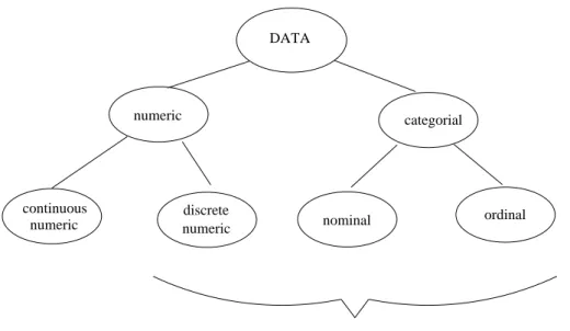
4.2.2 Basic data types . . . 43
4.2.3 Static and temporal data . . . 46
4.3 Properties of educational data . . . 47
4.3.1 Data size . . . 47
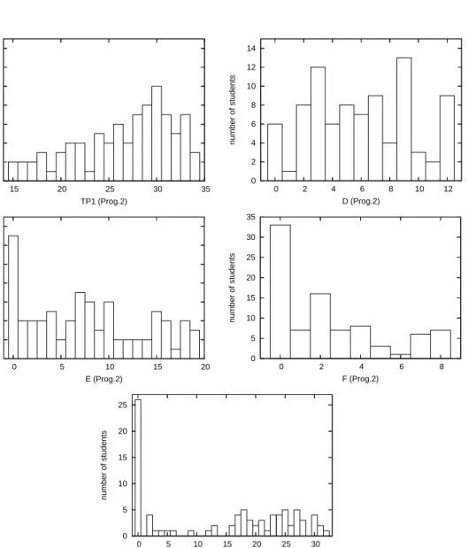
4.3.2 Data distribution . . . 50
4.4 Preprocessing data . . . 53
4.4.1 Feature extraction . . . 54
4.4.2 Feature selection . . . 61
4.4.3 Processing distorted data . . . 63
5 Modelling dependencies between attributes 67 5.1 Dependencies . . . 68
5.2 Correlation analysis . . . 69
5.2.1 Pearson correlation coefficient . . . 69
5.2.2 Restrictions and extensions . . . 71
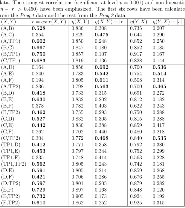
5.2.3 Pair-wise functional dependencies in ViSCoSdata . . . 73
5.3 Linear regression . . . 74
5.3.1 Multiple linear regression model . . . 74
CONTENTS 7
5.3.3 Multiple linear regression models for ViSCoSdata . . . 79
5.4 Discovering pair-wise statistical dependencies . . . 81
5.4.1 χ2-independence test and mutual information . . . . 82
5.4.2 Pair-wise statistical dependencies in the ViSCoSdata . . . . 83
5.5 Discovering partial dependencies by association rules . . . 85
5.5.1 Association rules . . . 86
5.5.2 Association rules in the ViSCoSdata . . . 88
5.6 Bayesian models . . . 89
5.6.1 Bayesian network model . . . 91
5.6.2 Bayesian models for the ViSCoSdata . . . 92
5.7 Comparison and discussion . . . 95
5.7.1 Modelled relations . . . 95
5.7.2 Properties of data . . . 96
5.7.3 Selecting the most appropriate method . . . 98
6 Clustering 99 6.1 Clustering problem . . . 100
6.2 Measures for distance and similarity . . . 102
6.3 Hierarchical clustering . . . 104
6.4 Partitioning methods . . . 110
6.5 Probabilistic model-based clustering . . . 112
6.6 Comparison of clustering methods . . . 117
6.7 Clustering the numericViSCoS data . . . 120
8 CONTENTS
7 Classification 127
7.1 Classification problem . . . 127
7.2 Tree models . . . 129
7.2.1 Decision trees . . . 129
7.2.2 Decision trees for the ViSCoS data . . . 132
7.3 Bayesian classifiers . . . 134
7.3.1 General Bayesian models vs. naive Bayes models . . . 134
7.3.2 Naive Bayes models for the ViSCoSdata . . . 136
7.4 Neural networks . . . 138
7.5 k-Nearest neighbour classifiers . . . 141
7.6 Comparison of classification methods . . . 143
7.7 Empirical comparison of classifiers for theViSCoS data . . . 145
8 Implementing adaptivity in learning environments 149 8.1 Adaption as context-aware computing . . . 149
8.2 Action selection . . . 151
8.2.1 Inferring the context and selecting the action separately . . 152
8.2.2 Selecting the action directly . . . 154
8.3 Utilizing temporal information in adaption . . . 156
8.3.1 Hidden Markov model . . . 156
8.3.2 Learning hidden Markov models from temporal data . . . . 158
8.3.3 Dynamic Bayesian networks . . . 159
9 Conclusions 163
Appendix: Basic concepts and notations 166
Chapter 1
Introduction
In all empirical science we need paradigms – good instructions and practices, how to succeed. Educational technology is still a new discipline and such practices are just developing. Especially paradigms for modelling educational data by knowledge discovery methods have been missing. Individual experiments have been made, but the majority of research has concentrated on other issues, and the full potential of these techniques has not been realized.
One obvious reason is that educational technology is an applied science and many other disciplines of computer science are involved. Most of the researchers in the domain have expertise in educational science, while few master machine learning, data mining, algorithmics, statistics, and other relevant disciplines. The other rea-son is domain-specific: the educational data sets are very small – the size of a class – and specialized techniques are needed to model the data accurately.
This thesis tries to meet this need and offer a wide overview of modelling paradigms for educational purposes. These paradigms concern both descriptive modelling – dis-covering new information in educational data – and predictive modelling – predicting learning outcomes. Special emphasis is put on selecting and applying appropriate modelling techniques for small educational data sets.
1.1
Motivation: modelling
ViSCoS
data
University of Joensuu has a distance learning program ViSCoS(Virtual Studies of Computer Science) [HSST01] which offers high-school students a possibility to study university-level computer science courses. The program has been very popular, but
2 CHAPTER 1. INTRODUCTION
the programming courses have proved to be very difficult and the drop-out and fail-ing rates have been large. To handle this problem, we have begun researchfail-ing ways to recognize the likely drop-out or failure candidates in time. This is valuable infor-mation for the course tutors, but also a critical element for developing adaptivity in the learning environment.
After discussing with ViSCoSteachers, we have defined the following goals for this research:
1. Identify common features for drop-outs, failed and skilled students:
Given the final results of the course, we should try to identify common fea-tures shared by drop-outs, failed and skilled students. As a sub-problem, we should discover whether these students fall into any homogeneous groups.
2. Detect critical tasks which affect course success:
Given the task points and final results, we should identify tasks that indi-cate drop-out, failure or excellent performance. It is possible that the tasks contain some ”bottle-neck” tasks, which divide the students.
3. Predict potential drop-outs, failed or skilled students:
Given the exercise task points in the beginning of course, we should predict who will likely drop out, fail or succeed excellently. The predictions should be made as early as possible, so that the tutoring could be adapted to stu-dent’s needs. Predicting the drop-outs and failed students is the most critical, because they should be intervened immediately. However, specially skilled students would also benefit from new challenges.
4. Identify the skills measured by tasks:
Given the course performance data, we should try to identify the skills mea-sured by the exercise tasks. According to course designers, the tasks measure different skills, but such evaluations are always subjective. As a modest goal, we could at least try to find groupings of tasks.
5. Identify student types:
Given the task points and grouping of tasks, we should try to discover, if the students fall into any clear groups. Supposing that the task groups measure different skills, we can further study the relations between skills and course results.
In the following chapters, we will process this problem further. We will define the modelling goals, select the appropriate modelling paradigms, analyze the available data, preprocess it and finally construct various models.
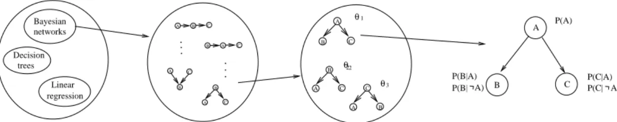
1.2. RESEARCH METHODS AND CONTRIBUTIONS 3 Bayesian networks Decision trees Linear regression A B C A B C A B C C A B A C B Modelling paradigms Model family Model class A B C P(B|A) P(B| A) P(C|A) P(C| A) P(A) Model . . . . .. 2 A B C B C A θ θ θ 1 2 3
Figure 1.1: The hierarchy of modelling concepts with examples from Bayesian net-works.
1.2
Research methods and contributions
The main problem of this research is to develop general principles for modelling educational data. This probelm can be divided into five subproblems (the concepts are defined in Table 1.1 and illustrated in Figure 1.1):
1. Selecting the modelling paradigm.
2. Defining the model family: the set of possible model structures is restricted by defining the variables and optionally some constraints on their relations. 3. Selecting the model structure: the optimal model structure is learnt from data
or defined by an expert.
4. Selecting the model: the optimal model parameters are learnt from data. 5. Validation: the descriptive or predictive power of the model is verified. The scientific paradigm in computer science contains general principles how to per-form optimally in each of these subproblems. However, each domain has its own requirements and restrictions. The general principles should be applied and revised and new principles created according to domain-specific needs. In educational tech-nology, such principles have been missing. This is exactly the goal of this research. First we should determine the specific requirements and restrictions of data mod-elling for educational purposes. Then we should select, apply and revise the existing modelling principles for our needs.
The principles proposed in this thesis have been derived from three components (Figure 1.2): general modelling principles, and the specific requirements and re-strictictions in educational technology.
4 CHAPTER 1. INTRODUCTION
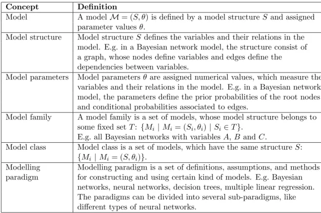
Table 1.1: The basic concepts concerning modelling.
Concept Definition
Model A model M= (S, θ) is defined by a model structure S and assigned
parameter valuesθ.
Model structure Model structure S defines the variables and their relations in the
model. E.g. in a Bayesian network model, the structure consist of a graph, whose nodes define variables and edges define the
dependencies between variables.
Model parameters Model parameters θ are assigned numerical values, which measure the
variables and their relations in the model. E.g. in a Bayesian network model, the parameters define the prior probabilities of the root nodes and conditional probabilities associated to edges.
Model family A model family is a set of models, whose model structure belongs to
some fixed set T: {Mi |Mi= (Si, θi) |Si∈T}.
E.g. all Bayesian networks with variablesA,B and C.
Model class Model class is a set of models, which have the same structure S:
{Mi |Mi = (S, θi)}.
Modelling Modelling paradigm is a set of definitions, assumptions, and methods
paradigm for constructing and using certain kind of models. E.g. Bayesian
networks, neural networks, decision trees, multiple linear regression. The paradigms can be divided into several sub-paradigms, like different types of neural networks.
1.2. RESEARCH METHODS AND CONTRIBUTIONS 5 in educational technology Requirements principles General modelling Restrictions technology in educational
Modelling principles for educational technology
Figure 1.2: The main components of the research.
The main requirement in educational systems is that the model is robust, i.e. it is not sensitive to small variations in data. This is crucial, because the data changes often. The model should adapt to new students, new teachers, new exercise tasks or updated learning material, which all affect the data distribution. For the same reason, it is desirable that the model can be updated, when new data is gathered. A special requirement in educational technology is that the model is transparent, i.e. the student should understand, how the system models her/him (e.g. [OBBE84]). The main restrictions cumulate from educational data. According to our analy-sis, the educational data sets are typically very small – only 100-300 rows. The attributes are mixed, containing both numeric and categorial values. In additon, there are relatively many outliers, exceptional data points, which do not fit the general model.
Based on these assumptions, we have selected the most appropriate modelling paradigms for educational applications. We have applied them to ViSCoS data and created new methods for our needs. We have collected and derived several good rules of thumb for modelling educational data. All these principles are com-bined into a general framework for implementing adaptivity in educational systems in a data-driven way.
The main contributions of this thesis are the following:
Giving a general overview of possibilities and restrictions of applying knowl-edge discovery to educational domain.
Constructing a general framework for implementing adaptivity in learning systems based on real data.
6 CHAPTER 1. INTRODUCTION
Evaluation of alternative dependency modelling, clustering and classification techniques for educational purposes.
Constructing accurate classifiers from small data sets of ViSCoSdata for pre-dicting course success during the course.
Most of the methods have been implemented by the author. If other tools are used, they are mentioned explicitely.
Some of the results have been represented in the following articles:
H¨am¨al¨ainen, W.: General paradigms for implementing adaptive learning sys-tems [H¨am05].
H¨am¨al¨ainen, W., Laine, T.H. and Sutinen, E., H. Data mining in personalizing distance education courses [HLS06].
H¨am¨al¨ainen, W., Suhonen, J., Sutinen, E. and Toivonen, H. Data mining in personalizing distance education courses [HSST04].
H¨am¨al¨ainen, W. and Vinni, M.: Comparison of machine learning methods for intelligent tutoring systems [HV06].
The third article was accepted, but not published in the conference proceedings due to technical problems. The author has been the main contributor in all papers.
1.3
Organization
The organization of this thesis is the following: In Chapter 2, previous work on applying knowledge discovery techniques in educational domain is presented. In Chapter 3, we discuss about the general modelling principles and give guidelines for modelling educational datasets. In Chapter 4, typical educational data is analyzed and guidelines for feature extraction, selection and other preprocessing techniques are given. In Chapter 5, we evaluate the most appropriate dependency modelling techniques for educational data. In Chapter 6, the existing clustering methods for educational purposes are analyzed and our own clustering method is introduced. In Chapter 7, we analyze the suitability of existing classification methods for educa-tional data. The best methods are compared empirically with the ViSCoS data. In Chapter 8, a general framework for constructing an adaptive educational system from data is introduced. The final conclusions are drawn in Chapter 9. The basic concepts and notations are introduced in Appendix 9.
Chapter 2
Background and related research
In this chapter, we describe the main ideas of knowledge discovery and its appli-cations in educational technology. We report previous experiments on applying knowledge discovery methods in the educational domain.2.1
Knowledge discovery
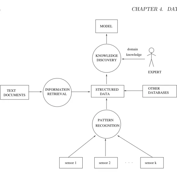
Knowledge discovery in databases (KDD), or briefly knowledge discovery, is a sub-discipline of computer science, which aims at finding interesting regularities, pat-terns and concepts in data. It covers various techniques from traditionally separated disciplines of machine learning, data mining and statistics. However, knowledge dis-covery is not just a combination of data mining and machine learning techniques, but a larger iterative process, which consists of several phases (Figure 2.1).
Understanding the domain is the starting point for the whole KDD process. We should understand both the problem and data in a wider context: what are the needs and goals, what kind of and how much data is in principle available, what policies restrict the access, etc. The preprocessing phase is often very worksome. We have to select suitable data sources, integrate heterogeneous data, extract attributes from unstructured data, try to clean distorted data, etc. The educational data exists in many forms and often we have to do some manual work. Discovering patterns is the actual data mining or machine learning task. Given a good preprocessed data set it is quite straight-forward, but often we have to process in a trial and error manner, and return back to prepare better data sets. In the postprocessing phase the patterns are further selected or ordered and presented (preferably in a visual
8 CHAPTER 2. BACKGROUND AND RELATED RESEARCH 1. Understanding domain 3. Discovering patterns 5. Application 2. Preprocessing data 4. Postprocessing results
Figure 2.1: Knowledge discovery process.
form) to the user. Finally, the results are taken into use, and we can begin a new cycle with new data.
In the current literature, concepts ”knowledge discovery”, ”data mining” and ”ma-chine learning” are often used interchangeably. Sometimes the whole KDDprocess is called data mining or machine learning, or machine learning is considered as a subdiscipline of data mining. To avoid confusion, we follow a systematic division to descriptive and predictive modelling, which matches well with the classical ideas of data mining and machine learning1. This approach has several advantages:
The descriptive and predictive models can often be paired as illustrated in Ta-ble 2.1. Thus, descriptive models indicate the suitability of a given predictive model and can guide the search of models (i.e. they help in the selection of the modelling paradigm and the model structure).
Descriptive and predictive modelling require different validation techniques. Thus the division gives guidelines, how to validate the results.
Descriptive and predictive models have different underlying assumptions (bias) about good models. This is reflected especially by the score functions, which guide the search.
1It matches also the division tounsupervisedandsupervised learningused in machine learning literature.
2.1. KNOWLEDGE DISCOVERY 9 Table 2.1: Examples of descriptive and predictive modelling paradigm pairs. The descriptive models reveal the suitability of the corresponding predictive model and guide the search.
Descriptive paradigm Predictive paradigm
Correlation analysis Linear regression Associative rules Probabilistic rules
Clustering Classification
Episodes Markov models
We will return to the interaction between descriptive and predictive modelling in Chapter 3. Now we will give a brief historical review of classical data mining and machine learning to illustrate the differences of these two approaches. The main differences are summarized in Table 2.2.
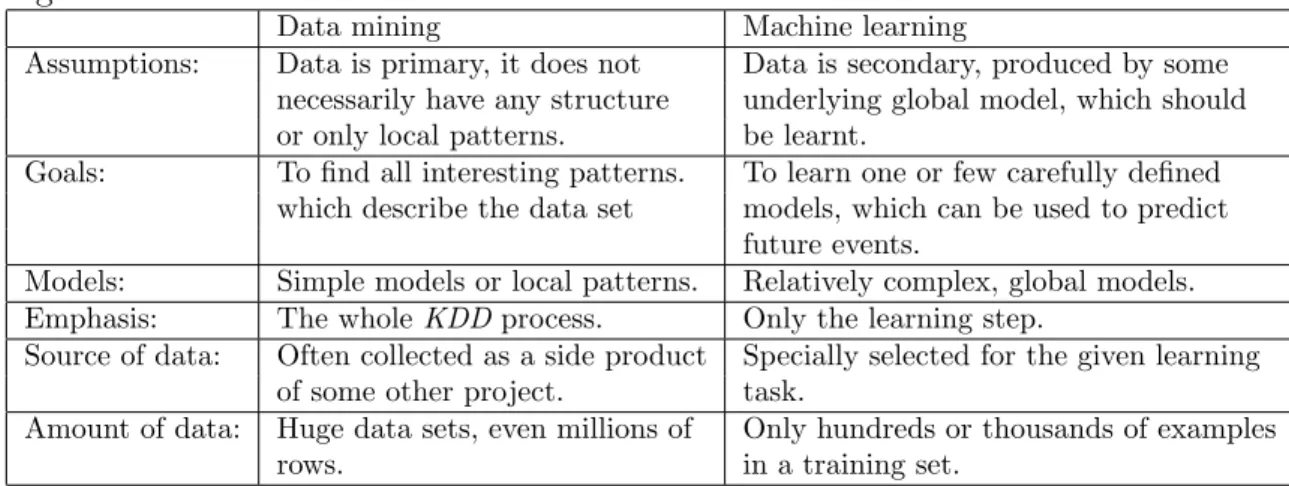
Table 2.2: Summary of differences between classical data mining and machine learn-ing.
Data mining Machine learning
Assumptions: Data is primary, it does not Data is secondary, produced by some necessarily have any structure underlying global model, which should or only local patterns. be learnt.
Goals: To find all interesting patterns. To learn one or few carefully defined which describe the data set models, which can be used to predict
future events.
Models: Simple models or local patterns. Relatively complex, global models. Emphasis: The wholeKDDprocess. Only the learning step.
Source of data: Often collected as a side product Specially selected for the given learning of some other project. task.
Amount of data: Huge data sets, even millions of Only hundreds or thousands of examples
rows. in a training set.
The main difference of data mining and machine learning concerns the goals of modelling and the underlying ontological (and epistemic) assumptions. In machine learning the main goal is to learn amodel, which can be used to predict future events. The underlying assumption is that there is a model, which has produced the data. The model is global, because it explains the whole data set, but more important is that it generalizes to new data. By contrast, in data mining, the main goal is to discover new interesting information which describes the current data set. Often, we do not even try to find global models, but only local patterns, which describe some parts of data. Now the data itself is primary, and we do not assume the existence of any models, before they are discovered. According to these emphases, the primary
10 CHAPTER 2. BACKGROUND AND RELATED RESEARCH
task of machine learning is called prediction task ormodel-first approach, while the primary task of data mining is called descriptive taskor data-first approach.
The other differences between machine learning and data mining are more practical. In machine learning, we can search more complex models, because the task is more focused. We want to learn only one or few carefully defined models, which predict the variable in question. In data mining, the task is less focused, because we want to discover all interesting patterns. The patterns are usually quite simple, because we have no a priori assumptions what kind of patterns to search, and we have to try all possible patterns. In addition, the data sets in traditional data mining are huge, and we could not search complex models efficiently. Typically, the origin of data sets is also different: in machine learning, the training set has been specially selected for the learning task, while in data mining, the data may be originally collected for some other purpose.
Both data mining and machine learning owe a great deal to statistics, and many new ideas have born in the interaction between the disciplines. Data mining and machine learning have naturally more emphasis on computational issues and they have been able to develop efficient search methods for complex models (machine learning) and exhaustive search in large data sets (data mining). The volume of data can be seen as one difference, although both data mining and machine learning methods can be applied to small data sets, as well, as we will demonstrate in this thesis. Statistics has also an important role in validation of results both in data mining and machine learning. This topic is further discussed in Chapter 3.
2.2
Knowledge discovery in educational
technol-ogy
One of the main main goals of educational technology is to adapt teaching to in-dividual learners. Every teacher knows that learning is most effective, when the teacher knows all her/his students and can differentiate the teaching to their indi-vidual needs. In large classes and distance learning this is not possible, and new technology is needed.
In the simplest form, a learning system gives the teachers more information about students. For example, in our ViSCoS project, the most acute need is to predict potential drop-outs and failing students as early as possible. The actual tutoring actions are left for the teacher’s responsibility. In the other extreme are intelli-gent tutoring systems (ITS) (see e.g. [dB00, KV04, CCL03, Was97, Web96, SA98,
2.3. RELATED RESEARCH 11 CHZY03]), where the whole tutoring is automated. This is achieved by two compo-nents: a student model and a tutoring module. The student model consists of a set of features describing the student’s current state. Typically, it contains cognitive information (knowledge level, prerequisite knowledge, performance in tests, errors and misconceptions), user preferences (learning style, goals and habits), action his-tory, and maybe some additional information about learner’s attitudes, emotions and motivation. Some features can be directly observed, but most of them are derived from observations. Given the student model, the tutoring module selects the most suitable actions according to some rules. These actions involve generat-ing tests and exercises, givgenerat-ing hints and explanations, suggestgenerat-ing learngenerat-ing topics, searching learning material and collaborative partners, etc.
The problem of current intelligent tutoring systems is that they are stable. The student model and actions are usually determined by fixed rules. Even if more sophisticated methods like Bayesian networks are used, the model is predefined by the system designers. According to our literature review, none of the existing intelligent tutoring systems learns the model from real student data. Thus, the adaptivity of such systems means that the students are adapted to some existing model or theory, instead of adapting the model to reality of students.
Implementing the whole intelligent tutoring system based on real data can be im-possible. The available data sets are very small, typically the size of a class, and complex models cannot be learnt accurately from data. However, half-automated learning systems or elements of adaptive learning environments can be learnt from data. In simple, single-purpose systems we can collect large amounts of data, be-cause the same task occurs again and again in different variations. This data can be used to learn a model, which predicts the student’s success in the next task, for ex-ample the next error ([MM01]) or the next help-request ([BJSM03]). The student’s general knowledge level can be approximated by her/his expected course score. In a coarse level (e.g. fail/success), the score can be predicted quite accurately already in the beginning of course ([KPP03]). The students’ typical navigation paths in the learning material can be analyzed and used to suggest appropriate material for new students ([SB03]). The students’ knowledge-level errors or misconceptions can be revealed by analyzing their solutions ([SNS00]). This is important information for the teachers, but also for automatic feedback generation.
2.3
Related research
Current adaptive educational systems are very seldom based on real data. However, there has been some research to this direction. To get a complete picture of the
12 CHAPTER 2. BACKGROUND AND RELATED RESEARCH
current state of affairs, we have performed a meta-analysis on research literature addressing either predictive or descriptive modelling on educational data. For this review, we have systematically checked all proceedings of Intelligent Tutoring Sys-tems and volumes of International Journal of Artificial Intelligence in Education since 1998. In addition, we have searched papers in ACM, IEEE and Elsevier dig-ital libraries with appropriate keywords, and checked all relevant references. This massive search resulted over 100 candidate papers, which promised to apply ma-chine learning, data mining or other intelligent techniques on educational data, but only 23 of them described actual experiments using real data. 15 of them address predictive modelling and the rest 8 descriptive modelling.
2.3.1
Predictive models learnt from educational data
In Table 2.3, we have summarized all experiments, which have learnt predictive models from educational data. In some cases, the data was artificially generated, and the applicability to real data remained uncertain.
Predicting academic score or success in studies
In the first five experiments the goal was to predict the academic score or success in studies.
In [KPP03], drop-out was predicted based on demographic data (sex, age, mari-tal status, number of children, occupation, computer literacy, job associated with computers) and the course data in the first half of the course (scores in two writing assignments and participation to group meetings). Six classification methods (naive Bayes, decision tree, feed-forward neural network, support vector machine, 3-nearest neighbour and logistic regression) were compared with different attribute sets. All the methods achieved approximately the same accuracy. In the beginning of the course, given only demographic data, the accuracy was 63%, and in the middle of the course, given all attributes, it was 80%. Naive Bayes classifier achieved the best overall accuracy, when all results in all test cases were compared.
In [MBKKP03], the goal was to predict the course score, but now the drop-outs were excluded. The data was collected from the system log and contained attributes con-cerning each task solved (success rate, success at first try, number of attempts, time spent on the problem, giving up the problem, etc.) and other actions like participat-ing in the communication mechanism and readparticipat-ing support material. Six classifiers (quadratic Bayesian classifier, 1-nearest neighbours, k-nearest neighbours, Parzen window, feed-forward neural network, and decision tree) and their combination were
2.3. RELATED RESEARCH 13 T able 2.3: Summary of exp erimen ts whic h ha ve learn t predictiv e mo dels from educational data. Abbreviations for the most common metho ds are: DT= decision tree, BN = Ba yesian net w ork, NB= naiv e Ba yes classifier, FFNN= feed-forw ard neural net w ork, SVM= supp ort vector mac hine, k -NN= k -nearest neigh b our classifier, LR=logistic regression. In V alidation field, the validation metho d (CV= cross-v alidation, TS=test set) and the b est accuracy (classification rate) are rep orted. In some exp erimen ts, other validation metho ds and accuracy measures w ere used. Reference Predicted attribute Other attributes Data size Metho ds V alidation [KPP03] Drop-out (binary) 11 Demographic, 350 NB,DT, FFNN, SVM, TS, 83% course activit y 3-NN, LR [MBKKP03] Course score 6 Solving history 227 quadratic Ba yes, 1-NN, CV, 87% (binary) in previous tasks k -NN, P arzen windo w, FFNN, DT, com bination [ZL03] Course score 74 Demographic, 300 Bo osting w eak TS, 69% (binary) preferences, habits classifiers [BTR04] Graduating in 6 56 Demographic, > 5000 FFNN, SVM CV, 63% years (binary) academic, attitudinal [ML W + 00] Need for remedial Demographic, earlier ab out 600? Asso ciation rules TS, precision 47%, classes (binary) sc ho ol success classifier, NB recall 91% [BW98] Time sp en t to solv e 25 Concerning problem 1781 FFNN CV, SSE 33% smaller a problem (n umeric) typ e, studen t’s abilities than in random guess [BJSM03] W ords, where the 20 Concerning w ord, 550 000 w ords DT, NB TS? 75% studen t asks help studen t, learning history 53 studen ts [MM01] The next errors Error typ es in previous 3300 BN TS, co efficien t of answ ers (categorial) determination r 2= 0 . 75 [JJM + 05] Mastering a skill Previous answ ers, and 360 (sim ulated HMM Mo del parameters (binary) whether a hin t w as studen ts) w ere compared to sho wn (binary) actual ones [V om04] Mastering a skill Previous answ ers 149 BN CV, correctly (binary) classified skills [DP05] T est score (binary) Answ ers to test 48+41 BN variation CV, compared to LR questions (binary) (2 courses) [CGB03] Appropriate material 5 Concerning learning 400+800 Adaptiv e Ba yes TS 200+400, 89% for a studen t st yle, material typ e sim ulated data [SB03] In teresting material Last h tml pages visited, 30 studen ts, Clustering, a variation Studen t feedbac k for a studen t keyw ords in eac h page 133 pages of DT [CF04] Optimal emotional P ersonalit y typ e 137 Probabilistic rules, Not rep orted state for learning (categorial) DT [SGMM03] Error or Log data? sim ulated data, FFNN Not rep orted misconception size not rep orted
14 CHAPTER 2. BACKGROUND AND RELATED RESEARCH
compared. When the score variable had only two values (pass/fail), the accuracy was very good. The combination of classifiers achieved 87% accuracy, and the best individual classifier, k-nearest neighbours, achieved 82% accuracy. The accuracy was further improved by optimizing the combined classifier by genetic algorithms, but now only training error was reported.
In [ZL03], the approach was very similar: to combine several weak classifiers by boosting to predict the final score. However, now the data was gathered by a questionnaire. In addition to demographic data, it contained attributes concerning the student’s network situation, surfing habits, teaching material applications, on-line learning preferences and habits, overall opinion of the course, etc. Each weak classifier used only one of 74 attributes to predict the course score. The combination achieved only 69% accuracy. However, the boosting revealed the most influencing factors for the course success.
In [BTR04], the goal was to predict, whether the student graduates in six years. The data was gathered by a questionnaire, and contained 56 demographic, academic, and attitudinal attributes. Feed-forward neural networks and support vector machines were learnt from the data. Both methods achieved only 63% accuracy, despite of the large data set (over 5000 rows). In addition, feature selection by principal component analysis only decreased the accuracy.
In [MLW+00], the goal was to select students, who would need remedial classes. The selection was made by comparing the predicted average course score in the next semester to some threshold. The data was described only vaguely (demographic data and school success in the previous year). The authors applied their own classification method, described in [LMWY03]. The idea was to search all association rules, which could be used for predicting the final score. In classification, all relevant rules were applied and a score was calculated based on rule confidences and frequencies. The method was compared to naive Bayes and decision tree classifiers by calculating precision and recall measures. The new method outperformed both naive Bayes and decision trees, although the precision was still low (47%). The problem in this research was that some students had actually participated remedial classes, but their success was estimated as they had been in the normal classes.
How the student succeeds in the next task?
The next four experiments concerned how to predict the student’s success, errors or help request in the next task given data from the previous tasks. All experiments were based on data collected from a real educational system. The systems had been specialized to one simple task type, which was repeated in different variations. Thus, large data sets could be gathered for training.
2.3. RELATED RESEARCH 15 In [BW98], neural networks were used to predict the time spent in solving an exercise task. Each task concerned basic arithmetic operations on fractions. The data set contained beliefs about student’s ability to solve the task, the student’s average score in required sub-skills, the problem type and its difficulty, and the student’s gender. First, a group model was learnt from the whole data. In cross-validation, the model achieved 33% smaller SSE compared to a random guess. Next, the model was adapted to each individual student by setting appropriate weights. Now 50% smaller SSE was achieved, compared to a random guess, but it was not clear, whether these results were validated.
In [BJSM03] a system for teaching pupils to read English was used. The goal was to predict on which word the student asks help. The data set contained student information (gender, approximated reading test results of the day, help request behaviour), word information (length, frequency, location in the given sentence) and the student’s reading history of that word (last occurrence, how many times read, average delay before reading, etc.). Only the poor students’ data was selected, because they ask help most frequently. First, a group model was learnt from all data and then the model was adapted using individual students’ data. Two classifiers, naive Bayes and decision trees were compared. The group models were presumably validated by a separate test set. (The authors tell that they could use only 25% of data for training because of technical problems.) Naive Bayes achieved 75% accuracy and decision trees 71% accuracy. When individual models were compared, only the training errors were reported. Now decision trees performed better, with 81% accuracy. When the information about graphemes (letters or letter groups) in words was taken into account, the accuracy increased to 83%.
In [MM01], a system for learning English punctuation and capitalisation was used. The task was to predict the errors (error types) in the next task, given the errors in the previous tasks. A correct answer should fulfill certain constraints, and each broken constraint corresponded to an error type. The system contained 25 con-straints, which occurred in 45 problems. 3300 records log data was collected, when the system was in test use.
A bipartite Bayesian network was used to represent the relationships between con-straints in the previous and the next tasks. Given this general form of a graph structure, both the model structure and parameters were learnt from data. This group model was adapted to the individual student, by updating the conditional probabilities after every task. The group model was validated by a separate test set. The coefficient of determination, which described the number of correctly predicted constraints as a function of the number of all relevant constraints, was r2 = 0.75. The individual models could not be validated (there was continual training), but they had a positive effect on the students’ scores.
16 CHAPTER 2. BACKGROUND AND RELATED RESEARCH
Computerized adaptive testing
Some researchers have considered the problem of estimating the student’s knowledge (mastering a topic), given a task solution (correct or incorrect). This is an important problem inITSs, but also in computerized adaptive testing (CAT), where we should select the next question according to the student’s current knowledge level. The problem in defining probability P(T opic = mastered|Answer = correct) is that we cannot observe mastering directly. Even if the task measures only one skill, the student can guess a correct answer or make a lapse. In practice, the tasks usually measure several inter-related skills. The next experiments introduce data-driven solutions to this problem.
In [JJM+05], the goal was to predict, whether a student answers correctly to the next task, given the previous task solutions (correct or incorrect) and information, whether a hint was shown. It was assumed that each task measures only one skill. For each skill, a hidden Markov model was created. Each Markov model contained a sequence of hidden state variables (mastering a skill), connected to observation variables (answer and hint). All variables were binary. Artificial data of 360 stu-dents was generated, assuming some model parameters. The data was used for model construction and the parameters were compared. All conditional probabili-ties could be estimated correctly with one decimal precision. However, most of the probabilities were just 0 or 1, based on unrealistic assumptions (e.g. a skill could not be mastered, if no hints were shown).
In [Vom04], the same problem was solved by a Bayesian network. The data was gathered from 149 students, who solved questions on arithmetic operations on frac-tions. The tasks tested 19 skills and seven error types were discovered in students’ solutions. The relevant skills and error types for each task were analyzed. Then a Bayesian network which described the dependencies between the skills was learnt from data. Some constraints like edges and hidden nodes were imposed according to the expert knowledge. Finally, the model parameters were learnt from the data for the best model structures. The models were compared by cross-validation. In each model, the states of skills (mastered or non-mastered) were determined after each task. The differences were very small, and nearly all models could predict correctly 90% of skills after nine questions.
In [GC04], the problem was solved in a more traditional way, based onitem response theory (IRT) [Lor80]. The probability that a student with certain knowledge level answers the item correctly was described by anitem characteristic curve. In [GC04], the item characteristic curve was estimated by a logistic function. The parameters were determined experimentally, but the parameters could be learnt from data, as well.
2.3. RELATED RESEARCH 17 In [DP05], a new variation of belief networks was developed. It was assumed (unre-alistically) that all dependencies were mutually independent, i.e.P(Y|X1, ..., Xk) =
Q
iP(Y|Xi), where Xis are Y’s parent nodes. With this simplification the model
structure could also be learnt from data, by determining the binary conditional de-pendences. The model was compared to a traditionalIRTsystem, where the logistic regression parameters were also learnt from data. The evaluation was based on the number of questions needed to classify the examinees as mastering or non-mastering the topic. This was determined by comparing the estimated final score to a given threshold value. Real data from two courses was used to simulate adaptive ques-tioning process. In the first data set, both methods could classify correctly over 90% of examinees after 5-10 questions, but in the second data set the new method performed much better. It could classify over 90% of examinees correctly after 20 items, while the traditional method required nearly 80 items.
Individually recommended material for students
The problem of adapting learning material or guiding the navigation in www ma-terial is speculated in several sources (e.g. [Bru00, Sch98]). Most systems use fixed rules, but the ideas of general recommendation systems can be easily applied to educational material. However, the underlying idea of recommending similar ma-terial for similar users is not necessarily beneficial in the educational domain. The students should be recommended material, which supports their learning, and not only material which they would select themselves. In the following two experiments the recommendations were learnt from real data.
In [CGB03], the goal was to recommend students the most appropriate material according to their learning style. The material was first preselected according to its difficulty and the student’s knowledge level. The student’s learning style was defined by a questionnaire, which measured three dimensions (visual/verbal, sensing/conceptual, global/sequential). The material was characterized by two at-tributes, learning activity (explanation, example, summary, etc.) and resource type (text, picture, animated picture, audio, etc.). A variation of naive Bayes, called adaptive Bayes, was used for predicting the most appropriate material, given learn-ing the style and material attributes. The model was otherwise like a naive Bayes, but the conditional probabilities were updated after each new example. The idea was that all actually visited pages were interpreted as appropriate material. The model was compared to traditional naive Bayes and an adaptive Bayes with fading factors, where smaller weights were given to older examples. The test data con-sisted of two simulated data sets, where students’ preferences changed 2-3 times. The best results (89% training error) were achieved with an adaptive Bayes using
18 CHAPTER 2. BACKGROUND AND RELATED RESEARCH
fading factors.
In [SB03], the goal was to recommend interesting www pages for students. Now the recommendations were based on keywords that occurred in the pages. First, the last 10 pages visited by the student were clustered according to their keywords. The cluster with the most recent page was selected and a decision tree was learnt to classify new pages into this cluster. The authors developed a new version of the classical ID3 decision tree algorithm, which created decision trees in three dimen-sions. In the new SG-1algorithm, several decision trees were created, when several attributes achieved the same information gain. The method was tested with real students, but the students followed the recommendations rarely and argued that the system suggested irrelevant links. The problem was further analyzed by clus-tering all 133 pages according to their keywords. The clusclus-tering revealed one large, heterogeneous cluster as a source for unfocused recommendations.
Other work
The last two experiments in the table are very vaguely reported, and not validated. In [CF04], the goal was to determine the most optimal emotional state for learning, given the student’s personality type. 137 students answered a questionnaire, which determined their personality type (extraversion, people with high lie scale, neuroti-cism, psychoticism), and selected their optimal emotional state from 16 alternatives. The authors reported that they used naive Bayes classifiers for rule construction, but in fact they just used the same parameter smoothing technique which is used in estimating parameters for Bayesian networks. In addition, they reported that they could learn the current emotional state from a colour series by decision trees with 58% accuracy, but no details were given.
In [SGMM03], the goal was to diagnosize the student’s errors and misconceptions related to basic physics. The data was collected with a simulation tool, where students were asked to draw gravitation and contact forces, which affect the given objects. The teacher planned a set of simulated students and determined their knowledge levels in different categories. In addition, each student’s behaviour was described by some fuzzy values. Then a feed-forward neural network was trained to classify the errors. 87% training accuracy was achieved, but the results were not validated.
In addition, there has been some general discussion, how to apply machine learn-ing methods in educational technology. For example, [LS02] discusses in a very superficial level, how to apply machine learning in intelligent tutoring systems.
2.3. RELATED RESEARCH 19
2.3.2
Descriptive models searched from educational data
Descriptive data modelling techniques (other than basic statistics) are more sel-domly applied to educational data than predictive techniques. One reason may be that data mining is still quite a new discipline. In Table 2.4, we have summarized all experiments, which have searched descriptive models from educational data. Some of the methods could be used for predictive modelling as well, but the intention has been descriptive analysis. For example, decision trees are often used to discover decision rules. These rules are interpreted – and sometimes even called – as asso-ciation rules. However, this is misleading, because the decision rules can be very rare (i.e. non-frequent) and decision trees reveal only some subset of rules affecting the class variable. The reason is that the decision tree algorithms find only a local optimum and sometimes the attributes are selected randomly. Thus, a full search of real association rules should be preferred.Analyzing factors which affect academic success
The first three researches in the Table analyze the most influencing factors on aca-demic success or failure (acaaca-demic average score or drop-out).
In [SK99], the factors which affect average score and drop-out among distance learn-ers were analyzed. The data was collected by a questionnaire. The questions con-cerned job load, social integration, motivation, study time, planned learning, and face-to-face activities. First, all correlations were analyzed, and a path model was constructed. According to this model, the most influencing factors on average score were study time, planned learning and face-to-face activities. In the second exper-iment, a logistic regression model for predicting drop-out (enrollment in the next semester) was constructed. Now social integration and face-to-face activities were the most significant factors.
In [SAGCBR+04], a quite similar analysis was performed. The task was to ana-lyze the factors which affect academic average mark, desertion and retention. The data set consisted of nearly 23 000 students, described by 16 attributes, including age, gender, faculty, pre-university test mark, and time length of stay at univer-sity. First, the dependences were determined by regression and contingency table analysis. Then the data was clustered, resulting 79 clusters. The clusters with the highest academic average score, the lowest academic average score, and the longest period of stay were further analyzed. Finally, decision rules for predicting good or poor academic achievement, desertion or retention were searched by C4.5 algorithm. The confidences of rules were determined and the strongest rules were interpreted.
20 CHAPTER 2. BACKGROUND AND RELATED RESEARCH T able 2.4: Summary of exp erimen ts whic h ha ve searc hed descriptiv e mo dels from educational data. Reference Goal A ttributes Data size Metho ds [SK99] F actors whic h affect score 20, concerning job load, 1994 Correlation, logistic and drop-out motiv ation, study time, activit y regression [SA GCBR + 04] F actors whic h affect academic 16, mostly demographic and 23000 Clustering, decision success/failure academic trees [BTR04] F actors whic h affect 6, demographic and attitudinal 100 Correlation, linear drop-out regression, discriminan t analysis [KB05] Na vigation patterns in log Action typ e, time-stamp, user, 1170 sessions Asso ciation rules, episo ds data target [R VBdC03] Relations b et w een kno wledge Kno wledge lev el, visited pages, 50 studen ts Asso ciation rules b y lev el in concepts and time sp en t time-stamps, success in tasks genetic algorithms on pages [MSS02] Grouping studen ts according T ask p oin ts 102 Clustering to skills [V C03] Disco vering dep endencies Studen t’s kno wledge in 15 436 Classification rules in questionnaire data topics, test score [SNS00] Analysis of kno wledge-lev el Erroneous Prolog programs 65+56 Clustering errors in studen ts’ solutions
2.3. RELATED RESEARCH 21 In [BTR04], only the factors which affect drop-out in distance learning were ana-lyzed. The data set consisted of 100 students, described by six attributes: age, gen-der, number of completed courses, employment status, source of financial assistance and ”locus of control” (belief in personal responsibility for educational success). The data was analyzed by correlation analysis, linear regression and discriminant analysis. The analysis revealed that the locus of control could alone predict 80% of drop-outs and together with financial assistance 84% of drop-outs.
Mining navigation patterns in log data
In adaptive hypermedia systems the main problem is to define recommendation rules for guiding students’ navigation in the learning material. One approach is to base these rules on students’ actual navigation patterns. The following two experiments have addressed this problem.
In [KB05], the aim was to find recommendation rules for navigation in hyperme-dia learning material. The data consisted of 1170 sessions of log data. For each action, the action type, time-stamp, user id, and target object (concepts and frag-ments) were recorded. 90% of data was used for the pattern discovery and 10% for verifying the results. In the first experiment, temporal order was ignored, and as-sociation rules between visited concept were discovered. In the second experiment, the temporal order was taken into account, and segmential and traversal patterns were discovered. Segmential patterns (serial episodes) described typical orderings between actions, which were not necessarily adjacent. In traversal patterns it was required that the actions were adjacent. The discovered patterns were used to pre-dict the actually visited concepts in the test data. Sequential patterns achieved the best accuracy, about 51%, but slightly better results were achieved when all pattern types were combined.
In [RVBdC03], a new way to discover interesting association rules in log data was proposed. The goal was to find relations between the student’s knowledge level in a concept, time spent to read material associated to that concept, and the student’s score in a related task. The data consisted of visited pages and timestamps, the student’s current knowledge level and success in tasks. The association rules were discovered by a new method based on genetic algorithms, where an initial set of rules was transformed by genetic operations, using a selected fitness measure. The method was tested in the course data of 50 students, and compared to the traditional apriori algorithm. The apriori algorithm worked faster and found more rules, as expected. However, the authors speculated that their method could find more interesting rules, because the fitness measure and other parameters could be selected according to modelling purposes.
22 CHAPTER 2. BACKGROUND AND RELATED RESEARCH
Analyzing students’ competence in course topics
Some researchers have made preliminary experiments to analyze students’ compe-tence in course topics, based on exercise or questionnaire task points. The problem in such an analysis is that a task can require several skills, but not in equal amounts. This is especially typical for computer science, where majority of knowledge is cu-mulative and interconnected. Some solution ideas have been discussed in [WP05]. [MSS02] described the first experiment to cluster data gathered in the ViSCoS project. The data consisted the weekly exercise points in Programming courses, but it was gathered earlier than our current data set. The goal was to cluster the students according to their points in different skills. The exercise tasks were analyzed and weights for 14 concepts were defined by experts. Because the task points were recorded on weekly basis, it was assumed that the students had got equal points in all tasks during one week. For each student, a weighed sum of exercise points in each skill was calculated and normalized to sum 1. Then the students were clustered to five groups by a probabilistic clustering method. The resulting clusters were analyzed by comparing the mean values of attributes and total skills in each cluster. It turned out that the individual skill means diverged only in the cluster of the poorest students (low total skills). In all other clusters no difference was found, but the grouping was simply based on total skills.
In [VC03], the students’ questionnaire answers were analyzed by ”association rules”. In fact, the rules were simple decision rules learnt by C4.5 algorithm, and only the rule confidences were reported. The data set consisted of 436 students, whose knowledge in 15 topics and final scores were given. The topic values were deter-mined according to related question answers. However, the same topic could be covered in several questions, and thus several data rows, one per each possible an-swer combination, were generated for each student. The final score was simply the sum of questionnaire points, classified as good, average or poor. A decision tree was learnt to predict the student’s final score, given her/his skills in topics, and decision rules were extracted from the tree. The training error was about 12%. However, both the topic attributes and final scores were derived from the same attributes, and the dependency was trivial.
Analyzing students’ errors in program codes
[SNS00] described a method for identifying knowledge-level errors in students’ er-roneous Prolog programs. The motivation was that the method could be used to construct an error library and assist in student modelling.
2.3. RELATED RESEARCH 23 The described method worked in two phases. First, the student’s intention (a cor-rect program, which the student has tried to implement) was identified. Then all erroneous programs with the same intention were hierarchically clustered to form an error hierarchy. The assumption was that the main subtrees in such a hierarchy corresponded to knowledge-level errors.
The method was tested in two simple programming tasks. In both tasks about 60 erroneous programs were achieved. The differences between programs were de-fined by the number of remove, add, replace and switch operations needed to transform a program to another. Clustering was implemented by two methods, ei-ther ignoring the error dependencies or using heuristic rules to model the causal relationships. The resulting cluster hierarchies were analyzed by experts, who had defined the knowledge-level errors in each program. The clustering with causal de-pendencies achieved clearly better results. In task 1, 84%, and in task 2, 70% of knowledge-level errors in students’ programs were detected. In task 1, 95%, and in task 2, 75% of discovered errors corresponded to real knowledge-level errors.
Other work
In addition, we have found a couple of small analyses, which were only vaguely reported. In [CMRE00], nine tutoring sessions with a human tutor were analyzed. The goal was to identify the discussion protocols and their changes. Decision trees were used to find rules which described the protocol changes. In [MLF98], a human expert’s problem solving paths were analyzed. A class regression tree was somehow used to identify the action sequences which led to success or failure. In [MBKP04], an idea for discovering interesting association rules from log data was proposed. A small experiment was made, but the results were not reported.
In [DSB04], it was discussed in a very general level, how educational systems could benefit from ”data mining” (both predictive and descriptive methods). In [HBP00], general ideas of applying web mining in distance learning systems were discussed.
Chapter 3
Modelling
The main problem in modelling educational data is to discover or learn robust and accurate models from small data sets. The most important factor which affects the model accuracy is the model complexity. Too complex models do not generalize to other data sets, while too simple models cannot model the essential features in the data. Model complexity has an important role in robustness, too, but there are several other factors which affect robustness. Each modelling paradigm and model construction method has its own inductive bias – a set of conditions, which guarantee a robust model. These conditions should be checked when we select the modelling paradigm, model structure, and model parameters.
In the following, we will first define the basic modelling terminology. Then we analyze the main factors – model complexity, inductive bias and robustness – which affect the model selection. We formulate principles for selecting an appropriate modelling paradigm and a model in the educational domain. Finally, we summarize the main techniques for model validation.
3.1
Basic terminology
The main problem of modelling is to find a model, which describes the relation be-tween target variable Y and a set of other variables, so called explanatory variables,
X. In all predictive tasks and most of the descriptive tasks, the target variable values t[Y] = y are given in the data. In machine learning, such tasks are called supervised learning, because the true target values ”supervise” the model search. In unsupervised learning, the target values are unknown, and the goal is to learn values which optimize some criterion. For example, in clustering we should divide
26 CHAPTER 3. MODELLING
all data points into clusters such that the clustering is optimal according to some criterion. In the following, we will concentrate on supervised modelling. We will return to clustering in Chapter 6
In data-driven modelling the models are learnt from a finite set of samples called a training set. Because the training set has only a limited size, we seldom find the true model, which would describe all possible data points defined in the relational schema. Thus, the learnt model is only an approximation.
Definition 1 (True and approximated model) LetRbe a set of attributes and
raccording toRa relation. LetX ={X1, ..., Xk} ⊆Rbe a set of attributes in Rand
Y ∈R the target attribute. Then the true model is a functionF :Dom(X1)×...×
Dom(Xk) → Dom(Y) such that t[Y] = F(t[X]) for any tuple t defined in R. The
approximated model is a function approximation M :Dom(X1)×...×Dom(Xk)→
Dom(Y) such that t[Y]≈M(t[X]) for all tuples t ∈r.
In machine learning literature (e.g. [Mit97][7]), true models are often called astarget functions, and approximated models ashypotheses. In the following, we will call the approximated models simply models.
In descriptive modelling, the models are often only partial, and we cannot define them by ordinary functions. However, we can define partial models by restrictions of functions:
Definition 2 (Partial model) Let R, r ∈ R, X ⊆ R and Y ∈ R be as before,
and r0 ( r. Model M is partial, if M|
r0 : Dom(X1)×...×Dom(Xk) → Dom(Y)
such that t[Y]≈M(t[X]) for all tuples t ∈r0.
The accuracy of the model is defined by its true error. The same error measure is used to measure how well the model fits the training set. Some examples of common error measures will be discussed in Section 3.7. The following definition is derived from [Mit97][130-131]:
Definition 3 (Training error and true error) Let d(M(X), Y) be an error
be-tween the predicted value M(X) and the real value of Y. Then thetraining error of model M in relationr, |r|=n, is
error(M, r) =
P
t∈rd(M(t[X]), t[Y])
3.2. MODEL COMPLEXITY 27 and the true error of model M is
errortrue(M) = lim
|r|→∞error(M, r).
If the true error is small, the model is called accurate. The relative accuracy mea-sures how well the model generalizes to new data.
If the error measure d is
d(M(X), Y) =
½
1, whenM(X)6=Y
0, otherwise
then the true error is the probability to make an error in prediction. Often we express the accuracy of the model as probability 1 −p, where p is the error probability. Notice that the true error is unobservable, although we can try to estimate it. We will return to this topic in Section 3.7.
In model selection, the main goal is to minimize the true error. Because the true error is unobservable, a common choice is to use some heuristic score function. Typically the score function is based on training error and some additional terms, which guide the search. An important criterion is that the score function is robust, i.e. insensitive to small changes in the data.
Given the score function, we can define the optimal model:
Definition 4 (Optimal model) Let M be a model,r a relation, and score(M, r)
a function, which evaluates the goodness of model M in relation r. We say that the model is optimal, if for all other models M0 6=M, score(M0, r)≤score(M, r). In many problems searching a globally optimal model is intractable, and the learning algorithms produce only a locally optimal model.
3.2
Model complexity
The desired model complexity is an important choice in model construction. On one hand, we want to get as expressive and well-fitting model as possible, but on the other hand, the more specialized the model is, the more training data is needed to learn it accurately.
28 CHAPTER 3. MODELLING
A special problem in educational domain is the small size of data. The smaller the training set is, the more the training error can deviate from the true error. If we select the model with the smallest training error, it probablyoverfits the data. The following definition is derived from [Mit97][67]:
Definition 5 (Overfitting) Let M be a model and r∈R a relation as before. We
say that M overfits data, if there exists another model M0 such that error(M, r)<
error(M0, r) and error
true(M, r)> errortrue(M0, r).
In overfitting the model adapts to the training data so well that it models even noise in the data and does not generalize to any other data sets. Overfitting can happen even with noise-free data, if it does not represent the whole population. For example, if a prerequisite test is voluntary, only the most active students tend to do it, and we cannot generalize the results to other students.
The best way to avoid overfitting is to use a lot of data. A small training set is more probably biassed, i.e. it does not represent the real distribution. For example, the attributes can have strong correlations in a sample, even if they are actually uncorrelated. When large amounts of data are not available, the best we can do is to select simple models. In practice, the attribute set can be reduced by selecting and combining original attributes. This is also an important option when selecting the modelling paradigm. Descriptive modelling paradigms impose usually very sim-ple patterns, but in predictive modelling, the paradigm may require too comsim-plex models. For example, decision trees require much more data to work than naive Bayes classifier. We will return to this topic in Chapter 7.
The other extreme, concerning model complexity, is to select too simple models. A simple model generalizes well, but it can be so general that it cannot catch any essential patterns in the data. We say that the model has weak representational power. Sometimes this phenomenon is called underfitting. It means that the model approximates poorly the true model or there does not exist any true model. In predictive modelling such a model causes poor prediction accuracy. In descriptive modelling it describes only trivial patterns, which we would know even without modelling. In descriptive modelling, this happens easily, because we perform an exhaustive search of all possible patterns. If we try enough many simple patters, at least some of them will fit the data, even if there are actually no patterns at all. As a compromise, we should select models which are robust and have sufficient representational power. Such models have the smallest true error and they are accurate. In practice, we should select simple models, which still explain the data well. Very often, this happens through trial and error, in an iterative process of descriptive and predictive modelling.