Do international portfolio investors follow firms’ foreign investment decisions?

WORKING PAPER SERIES

NO 815 /

SEPTEMBER

2007

DO INTERNATIONAL

PORTFOLIO INVESTORS

FOLLOW FIRMS’

FOREIGN INVESTMENT

DECISIONS?

by Roberto A. De Santis

ECB LAMFALUSSY FELLOWSHIP PROGRAMME

WORKING PAPER SERIES

NO 815 / SEPTEMBER 2007

In 2007 all ECB publications feature a motif taken from the €20 banknote.

DO INTERNATIONAL

PORTFOLIO INVESTORS

FOLLOW FIRMS’ FOREIGN

INVESTMENT DECISIONS?

1

by Roberto A. De Santis

2

and Paul Ehling

3

This paper can be downloaded without charge from http://www.ecb.int or from the Social Science Research Network electronic library at http://ssrn.com/abstract_id=1015266.

1 We would like to thank Gianni Amisano, Mihir Desai, and Christian Heyerdahl-Larsen, for very useful comments and valuable suggestions. Lars Kristian Klemo, Svein Petter Undheim, and Magnus Vågsether provided superb assistance with the data. We are grateful to Deutsche Bundesbank for making the FDI and FPI data available to us. Paul Ehling acknowledges the financial support of the Lamfalussy

ECB LAMFALUSSY FELLOWSHIP PROGRAMME

© European Central Bank, 2007 Address

Kaiserstrasse 29

60311 Frankfurt am Main, Germany

Postal address

Postfach 16 03 19

60066 Frankfurt am Main, Germany

Telephone +49 69 1344 0 Website http://www.ecb.europa.eu Fax +49 69 1344 6000 Telex 411 144 ecb d

All rights reserved.

Any reproduction, publication and reprint in the form of a different publication, whether printed or produced electronically, in whole or in part, is permitted only with the explicit written authorisation of the ECB or the author(s). The views expressed in this paper do not necessarily reflect those of the European Central Bank.

The statement of purpose for the ECB Working Paper Series is available from the ECB website, http://www.ecb.europa. eu/pub/scientif ic/wps/date/html/index. en.html

Lamfalussy Fellowships

This paper has been produced under the ECB Lamfalussy Fellowship programme. This programme was launched in 2003 in the context of the ECB-CFS Research Network on “Capital Markets and Financial Integration in Europe”. It aims at stimulating high-quality research on the structure, integration and performance of the European financial system.

The Fellowship programme is named after Baron Alexandre Lamfalussy, the first President of the European Monetary Institute. Mr Lamfalussy is one of the leading central bankers of his time and one of the main supporters of a single capital market within the European Union.

Each year the programme sponsors five young scholars conducting a research project in the priority areas of the Network. The Lamfalussy Fellows and their projects are chosen by a selection committee composed of Eurosystem experts and academic scholars. Further information about the Network can be found at http://www.eu-financial-system.org and about the Fellowship programme under the menu point “fellowships”.

CONTENTS

Abstract 4

Non-technical summary 5

1 Introduction 7

2 Models of FDI and FPI 9 2.1 A model of domestic and foreign

direct investment 10 2.2 A model of domestic and foreign

portfolio investment 13 2.3 Empirical implications 17 3 The data 20 4 Empirical results 22 5 Robustness checks 25 6 Conclusions 26 References 28 Appendices 31

Appendix : Figures and tables 35 European Central Bank Working Paper Series 43

Abstract:We analyze the interlinkages between foreign direct investment (FDI) and foreign portfolio investment (FPI) between Germany and the major economies. First, we show that Tobin’s q helps explaining the variation of the growth rate of the stock of FDI. Second, we show that foreign and the home stock market returns explain the variation of the growth rate of the stock of FPI. Most importantly, we find that information about foreign fundamentals is revealed via direct investment. In other words, FDI transactions measured by fitted growth rates of the stock of FDI help explaining current growth rates of the stock of FPI. To our knowledge this observation is the first unambiguous evidence that international portfolio investors follow firms’ expected foreign investment decisions.

JEL Classification Codes: F21, F23, G11, G15.

Key words: Foreign Direct Investment, Foreign Portfolio Investment, Tobin’s q, Investor Heterogeneity, and Information Spillovers.

Non-Technical Summary

Capital flow volume has grown at a phenomenal rate since the beginning of the 1990s. Given the extraordinary rise, economists acknowledge the influence of capital flows on the real side of the economy also of developed countries characterized by large market capitalizations. However, not much is known about the interlinkages between Foreign Direct Investments (FDI) and Foreign Portfolio Investments (FPI).

In this paper we analyze the joint determinants and joint dynamics of the growth rate of FDI and FPI between developed countries. We are especially interested in common driving forces for capital flows and in informational linkages.

Both our model and the empirical results suggest that the most important factor determining FDI and FPI transactions is the stock market. The stock market helps explaining FDI because it produces signals that are relevant for firm investments via q theory. Foreign stock market and home stock market determine FPI because they measure the investment opportunity set and wealth effects.

Managers of firms and portfolio investors ought to gather information about foreign countries. We argue that three possible outcomes of this information gathering are plausible: i) Firms follow swift and more knowledgeable portfolio investors. ii) Portfolio investors watch firms because firms have information about fundamentals that are not available to the public. iii) Firms and portfolio investors produce valuable information that is revealed by investment and, hence, firms and portfolio investors chase after each other.

We find that information about foreign fundamentals is revealed via direct investment. Accordingly, we do not detect any evidence for the argument that swift portfolio investors are the first to spot foreign investment opportunities. If there is any simultaneous link between equity FDI and equity FPI flows, we could not find it in the data.

How can international portfolio investors possibly follow direct investments, and utilize it for current portfolio choices, when FDI data is released with a lag?

Clearly, we must assume that portfolio investors understand the investment model of firms. Further, the input variables to the model need to be publicly known. Fortunately, in our model stock market data and lagged FDI data are sufficient. Our story is strongly supported by the empirics: Neither current FDI nor lagged FDI explain FPI, but fitted FDI from the empirical specification of our model does explain FPI.

Why are international portfolio investors interested in FDI dynamics?

Since domestic firms get hold of information about future demand on foreign markets it is likely that FDI dynamics are correlated with future aggregate foreign demand. Further, portfolio investors ought to learn about consumption streams on foreign markets. It turns out that it is beneficial to learn from two data sources because two time series speed up learning and reduce noise in the data.

To sum up, our analysis suggests that stock market development is the most important common driving force for FDI and FPI. Our analysis also suggests that international portfolio investors follow firms’ foreign investment decisions.

1. Introduction

In the last decade, capital flows attracted more interest by policy makers, central banks, international institutions and academia, mainly because flow volume has grown at a phenomenal rate since the beginning of the 1990s. Foreign Direct Investments (FDI) and Foreign Portfolio Investments (FPI) in particular have been growing worldwide. However, not much is known about the interlinkages between these two forms of investment.

In this paper we analyze the joint determinants and joint dynamics of the bilateral growth rate of the FDI and FPI stocks between Germany, the six remaining G-7 countries plus Switzerland. More specifically, we ask two vital questions: First, what is the common driving force of FDI and FPI flows? Second, are there any informational linkages between FDI and FPI activities?

Not surprisingly, we show that the most important factor determining FDI and FPI transactions is the stock market. Specifically, we find that home market Tobin’s q help explaining the growth rate of the stock of FDI. The q theory suggests that if expected profits of a firm increase and, as a result, the market value of a firm over its book value becomes greater than one, then the firm should increase its capital stock also abroad as investing is profitable1.We also find thatthe relative growth rate of the foreign market capitalization and home stock market return, determine the growth rate of the stock of FPI. The former measures the relative investment opportunity set and wealth effects in foreign markets, the latter controls for wealth effects in the home market.

Most importantly, we show that information about foreign fundamentals is revealed via direct investment and not via portfolio investment. In other words, FDI transactions help

1

Hayashi (1982) showed that if (1) the production function and the total adjustment cost functions are homogeneous of degree one (that is constant returns to scale), (2) the capital goods are all homogenous and identical, and (3) the stock market is efficient, then the shadow price qis equivalent to the ratio of the market value of a firm divided by the replacement cost of capital.

explaining the growth rates of the stock of FPI, while we find no evidence for firms acting on information generated by swift international portfolio investors.

Managers of firms and portfolio investors ought to gather information about foreign countries. Investment decisions based on past economic developments might not be necessarily appropriate. If firms’ marginal-q is expected to be correlated with future consumption (dividend) growth2, then learning about expected investment activity of multinational firms could have first order implications for portfolio choice. Overall, our empirical findings support this view.

Our paper is linked to the literature on the relation of stock market development (that is q-theory) and investments (Erickson and Whited, 2000, and Bond and Cummins, 2001). For example, Jovanovic and Rousseau (2002) show that mergers and acquisition in the US can be explained by the q-theory. More specifically, they find that mergers and acquisitions respond to stock market developments by more than direct investment. Similarly, Blonigen (1997) finds that the Japanese stock market is an explanatory variable of Japanese FDI in the United States in the late 1980’s and early 1990’s. In addition, De Santis, Anderton, and Hijzen (2004) find that Tobin’s q of the Euro area is a key determinant of FDI from the Euro area to the US. Our results are also interesting in light of Portes and Rey (2005), who find that stock market capitalization is a key driver of equity flows.

Albuquerque, Bauer, and Schneider (2006a) argue that heterogeneity within foreigners is more important in explaining international equity flows than heterogeneity of investors across countries. In a companion paper Albuquerque, Bauer, and Schneider (2006b) present empirical evidence for the argument that half of the variation in international equity portfolio flows may be explained by a common factor. Our findings can be interpreted as evidence for

2

Moner-Colonques, Orts, and Sempere-Monerris (2007) present a model where FDI resolves demand uncertainty, but exports do not.

the argument that this common factor is the stock market and that sophisticated portfolio investors learn from FDI activities.

Goldstein and Razin (2006) study a related issue. They develop a model of FDI and FPI to explain the first and second moments of capital flows under the hypothesis the FDI provides access to superior information. Moreover, they study the trade off between the stock of FDI and the stock of FPI based on the possibility of idiosyncratic liquidity shocks.

The plan of the paper is as follows. Section 2 contains the theoretical model of FDI based on Tobin’s q and the theoretical model of FPI based on investor heterogeneity. Section 3 shows the data. Empirical results are discussed in Section 4. Section 5 concludes. The Appendix sections offer technical details beyond those in Section 2.

2. Models of FDI and FPI

FDI activities are typically carried out by managers of firms, while decisions related to allocation of portfolios are taken by portfolio managers. Managers of firms aim at maximizing the present value of profits, while portfolio managers aim at maximizing the intertemporal utility function of their customers. Therefore, from the perspective of portfolio investors aggregate consumption is exogenous. Specifically, we assume that domestic (foreign) consumption, that is dividends, is the residual of domestic (foreign) output generated by domestic and foreign firms minus their new investment activity abroad and at home.

We also consider a channel of information transmission to connect the investment decisions of firms with the portfolio allocation decisions of portfolio investors. Developments in the stock market play a key role in initiating both direct and portfolio investments. Therefore, both models depend on the same fundamental information. However, information is assumed to be uncertain: for example, it may be difficult to interpret stock market news that have consequences for both types of new investments. Therefore, managers of firms and

portfolio investors will attempt to learn about the economy over time. This leads directly to the information based spillover that causes the models to interplay. We can think of three channels of information transmission between FDI and FPI: Firms and portfolio investors simultaneously learn or simultaneously receive information about fundamentals abroad and, thus, initiate FDI and FPI activities concurrently. Alternatively, portfolio investors could employ information generated by firms FDI activity as an input variable to their portfolio choice problem. Of course, it is also possible that portfolio investors are better informed or just act much faster than firms, possibly due to implementation costs at the firm level, and thus FDI follows the lead of portfolio investment decisions.

Our model does not rule out any of these interpretations for the flow of information and its impact on investments. As it will become clearer, these interpretations have testable empirical implications.

2.1. A Model of Domestic and Foreign Direct Investment

Assuming that capital depreciates at a constant proportional rate h, the evolution of the capital stock of a multinational firm is given by

t t t

t I FDI hk

k , (1)

where I_t denotes firm’s domestic investment, FDI_t firm’s FDI flows, k_t firm’s capital stock and a dot over a variable denotes the derivative of that variable with respect to time. A key feature of the production function is the “jointness” assumption (Markusen, 2002, Ch. 7). This property refers to the ability of using production inputs in multiple production locations without reducing the services provided in any single location. Skilled labor, blueprints, know-how, managerial services are all examples of joint inputs.

Under the purchasing power parity assumption (PPP), the net real cash flow, V_t , of a firm operating at home and abroad, net of labor costs, at time t is:

_{^ `}

³

f

¦

¦

» » ¼ º « « ¬ ª ¿ ¾ ½ ¯ ® ­ 1 1 2 1 2 2 , 2 t s n j js js s s s F n j js s F s s s D s D t s r t FDI p a ds k FDI a k G I k I k G e V G G (2) where D

G denotes the production function at home, F

G the production function in the host

country,

¦

n j jt a 1

the sum of all specific assets in the host country (e.g. resources, including the

monitoring of portfolio investment decisions by portfolio managers) priced at p_jt, G j the firm’s cost parameter of adjusting its capital stock, r the real interest rate, and j

D,F

denote domestic and foreign, respectively.

The firm chooses the paths of domestic investment and FDI by maximizing V_t subject to the evolution of the capital stock. Therefore, the current-value Hamiltonian is equal to

^

`

^ `

t t t

t n j js js s s s F n j js s F s s s I s D t t t hk FDI I q a p FDI k FDI a k G I k I k G FDI I k H » » ¼ º « « ¬ ª ¿ ¾ ½ ¯ ® ­

_¦

_¦

1 2 1 2 2 , 2 , , G G (3)

where q_t denotes the shadow value of the state variable (the value of a unit of capital). The first derivate with respect to the flows of n variable factor is:

0 js a F p G js . (4)

The derivatives of the Hamiltonian with respect to the control variables, It and FDIt,

yield the condition under which a firm invests to the point where the cost of acquiring capital equals the value of the capital:

t t t D q k I G 1 (5) t t t F q k FDI G 1 . (6)

Therefore, domestic and foreign investments are positive only when the shadow price

t

The derivative of the Hamiltonian with respect to the state variable, k_t, yields the condition under which the marginal revenue product of capital equals the opportunity cost of a unit of capital:

^ `

t t t s s F n j js t F k s s I t D k hq rq q k FDI a k G k I k G _¸¸ ¹ · ¨¨ © § ¿ ¾ ½ ¯ ® ­ ¸¸ ¹ · ¨¨ © §

_¦

2 1 2 2 , 2 G G . (7)

In words, owning a unit of capital for a period requires forgoing rq_t of real interest and involve offsetting gains of q_t.

Finally, the transversality condition lim 0 f

o t t

rt

t e qk states that the value of the capital

stock must approach zero.

Provided that permanent bubbles in the shadow price of capital are ruled out, so that 0

o

t

q as tof, the solution of the differential equation (7) yields the so-called marginal-q. That is, the value of a unit of capital at a given time equals the discounted value of its future marginal revenue products:

_ds k FDI G k I G e q t s s s F F k s s I D k t s h r t

³

f ¸ ¸ ¹ · ¨ ¨ © § ¸¸ ¹ · ¨¨ © § ¸¸ ¹ · ¨¨ © § 1 2 2 2 2 G G . (8)

As shown in Appendix A, marginal-q (8) corresponds to average-q (A1) under the hypothesis of constant returns to scale. However, if technology available abroad boost total factor productivity allowing increasing returns to scale, then additional factors that are host country-specific could further affect FDI decisions.

Assume that GD

^ `

k_t k1_tD and

E D ¸ ¸ ¹ · ¨ ¨ © § ¿ ¾ ½ ¯ ® ­

¦

¦

n j js t n j js t F a k a k G 1 1 1 , , then

D

D t D k k G 1 and

E D D _¸¸ ¹ · ¨ ¨ © §

¦

n j js t F k k a G 1

1 , where D denotes the output elasticity with respect to labor.

E ¸ ¸ ¹ · ¨ ¨ © §

¦

n j js D k F k G a G 1 . (9).

By using (8) and (9), (4) and (5) can be rewritten as follows:

» » ¼ º « « ¬ ª ¸ ¸ ¹ · ¨ ¨ © § ¸ ¸ ¹ · ¨ ¨ © §

³

f

¦

1 1 1 1 1 ds a G e k I t s n j js D k t s h r D t t E G (10) » » ¼ º « « ¬ ª ¸ ¸ ¹ · ¨ ¨ © § ¸ ¸ ¹ · ¨ ¨ © §

³

f

¦

_{1 1} 1 1 1 ds a G e k FDI t s n j js D k t s h r F t t E G . (11)

Equations (10 – 11) are independent and, therefore, we can focus our attention in the empirical implementation below on the FDI activity.3

All in all, the growth rate of FDI is function of the discounted value of the marginal product of capital as well as of the actual adjustment costs needed to increase the capital stock abroad. Moreover, the marginal product of capital is also a function of specific assets available abroad, such as technology, human capital and other resources, and may also be a function of the firm’s learning process from domestic portfolio investors about their international investment decisions.

2.2. A Model of Domestic and Foreign Portfolio Investment

Firms issues stocks that are held by country representative portfolio investors. Markets are assumed to be complete; therefore we abstract from currency risk. Investors are heterogeneous in endowments, beliefs about dividend and FDI growth, and risk aversion. We assume that investors learn over time by observing the dividends and other data such as FDI

3

This result is based on the hypothesis that multinational firms are not financially constrained. First, our approach is supported by the weak evidence that outward FDI competes with domestic investment found by Stevens and Lipsey (1991), who analyzed the interdependence between domestic and foreign investment when firms are financially constrained. Second, we look at developments among developed countries, which generally do not face liquidity constraints.

investments. It is important to stress that portfolio investors cannot observe dividend growth and marginal Tobin’s q of domestic, foreign or multinational firms. Moreover, they do not know the future foreign demand firms ought to satisfy. Therefore portfolio investors cannot anticipate real investment decisions, but may attempt to estimate it from publicly available information.

The dividend processes, D, associated with the stocks in the economy are modeled as continuous processes dD_jt D_jt

J_jtdtO_jtdW_jt

, where J are growth rates, O are volatility coefficients, and W are Brownian Motion terms of appropriate dimensions. These dividend processes should be interpreted as output after new investment, whether foreign or domestic, of the firms in the previous subsection. That is, the dividend processes, domestic and foreign, are functions of the production functions GD and GF. Since agents cannot observe , the dividend processes evolve as follows

>

i

@

jt j i jt jt jt D m dt dW dD O (12)

from the perspective of the investors, where i

D,F

denote domestic investor and foreign investor, respectively; and m represent dividend growth rates4 _{as perceived by the investors.}

Note that due to the fact that agents do not know the drift rate of the dividend processes they also do not observe the shocks to dividends, although agents agree on the observed current values of the two dividends. Therefore, the dividend processes are investor (country) specific, hence the i in the superscripts. In the remainder we assume that there is only one foreign country (investor). This is just to simplify notation, the structure of all equilibrium quantities are unchanged when more than two investors (countries) are present in the model.

Information spillovers from FDI markets may alter the way domestic investors perceive foreign dividend growth. Consider for example that the FDI growth rate in the

4

foreign country is correlated with or identical to the growth rate of the foreign dividend process. Then, domestic investors will follow FDI dynamics closely in order to learn about dividend growth. Although, the dynamics in Equation (12) and its structural form will not be altered by a more sophisticated learning process, the availability of this additional information channel will affect the perceived drift rates m. In words, the perceived drift rate of dividends in the foreign market will converge faster and with less noise to its true mean5_{. Therefore, it}

will be beneficial, in terms of consumption share, to the domestic investor to learn about foreign dividend growth by employing dividend and FDI dynamics.

For simplicity investors utility functions are of power type. Investors solve

» » ¼ º « « ¬ ª

³

f 0 1 1 maxE c dt i it t i c i i U E U s.t. ₀ 0 i it it i c dt X E _»d ¼ º « ¬ ª

³

f K (13)

where E are agent specific expectation operators (depending on the perceived dividend processes from above), E is the time preference, c is consumption, U is the constant risk aversion coefficient of the investors, K are agent specific state price densities, and X is the present value of endowment.

Solving Equation (13) and using the market clearing condition as well as the relation between investor (country) specific expectations lead to the following sharing rule for

aggregate consumption D F F Dt t F D Dt t c y y c D U U U [ / / 1 ¸¸ ¹ · ¨¨ © §

where D is aggregate dividends6_{, y}

are Lagrangian multipliers from agent’s first order conditions, and [ is the density process capturing the evolution of heterogeneity of beliefs over time.

5

Appendix C contains two formal examples that highlight the usefulness of a second –related– process for learning.

6

Clearly, in equilibrium all dividends are consumed and, therefore, aggregate dividends equal aggregate consumption.

To simplify the presentation of the model, we omit the construction of equilibrium and focus on optimal portfolio polices. Suppose the economy is in equilibrium7_{, then domestic and}

foreign portfolio investments are given by:

Dt t Dt

>

t i

@

Dt t it it X V T K V E \ H I 7 1 1 1 (14)

where X denotes the present value of wealth, V is the endogenous equilibrium covariance matrix of stock returns, T is the equilibrium Sharpe-Ratio from the domestic investors perspective, K is the domestic state price density, \ denotes the Malliavin derivative8_{, and}

H contains hedging terms against changes in the opportunity set. Both the Sharpe-Ratio and the state price density are affected indirectly by the perceived growth rate of dividends and possibly the growth rate of FDI. The first part of the portfolio policies (domestic and foreign) in Equation (14) is the growth optimal portfolio9_{. The second part of the optimal portfolio}

policies contains the hedging terms against fluctuations in the investment opportunity set10_.

The portfolio polices are expressed on the domestic probability measure, E_Dt. Since agents disagree on probabilities but agree on prices it is irrelevant on which measure the equilibrium quantities are obtained. The Appendix B contains the proof of Equation (14).

In the model heterogeneity in risk aversion and in prior beliefs, and learning from firms’ FDI activities lead to time variation of the equilibrium equity price processes that goes above and beyond the time variation in the underlying dividend processes. Consequently, the hedging terms in (14) are driven by aggregate risk aversion, the density process capturing the

7

A growing number of papers (see for instance Anders, et al. (2005), Chan and Kogan (2001), Constantinides and Duffie (1996), Dumas (1989), and Wang (1996) to name a few) analyze the implications of heterogeneous agents on asset prices and related topics. See also Detemple and Murthy (1994), Basak (2000), Williams (1977), Zapatero (1998) and Ziegler (2002) and the literature therein for dynamic equilibrium models with heterogeneous beliefs.

8

Malliavin calculus is a generalization of the calculus of variations (see Nualart, 1995).

9

See Merton (1969).

10

evolution of heterogeneity of beliefs, perceived dividend growth rates, and fluctuations in the dividend processes. The perceived dividend growth rates depend on priors, the path of the economy, and possibly on FDI dynamics. The hedging terms in H are of the following form:

_³

³

f f t s t is s t D is Ds D s t Ds s t Ds s t D Ds Ds D s i tH E u c c \ D c \ [ c ds E u c c \ D c \ [ ds \ [ [ ' '' (15)

where u denotes utility function, (.)’ and (.)’’ stand for first and second derivative, respectively; superscripts D and [ denote derivatives with respect to dividends and the heterogeneity of beliefs density process, respectively. Also when priors about growth are

Gaussian, _F Ž

^

1,2,3,4

`

D

U U

, the growth rates of the dividend processes are mean reverting, and

the dividend volatility coefficients are constants, then the domestic and foreign portfolio investments in Equations (14 – 15) are obtained in analytical form. The exact expressions of these hedging terms are available upon request.

Although, the form of Equation (15) is complex, the interpretation of it is simple: the hedging terms in the optimal portfolio policy appear because the investment opportunity set is time-varying. Each variable in the hedging term contributes to the time-variation in the investment opportunity set, e.g. future realizations of the Sharpe ratio.

All in all, the growth rate of portfolio investment at home and abroad is a function of aggregate risk aversion (derivatives of the utility function), expected Sharpe ratios (the latter terms cause the fluctuations in the investment opportunity set), and the wealth of the investor.

2.3. Empirical Implications

The direct implication of the model is that the growth rate of FDI is a positive function of the domestic market-to-book ratio (e.g. Tobin’s q11). Moreover, we predict a negative relation

11

between the growth rate of FDI and the lagged FDI stock, as the greater the capital stock abroad the larger would the adjustment costs be to increase it by a given rate.

As for the positive relation expected with host country-specific variables (such as future foreign developments in market size, technology, flexibility of the labor markets, other institutions, etc.) that will increase firms’ future output, we make use of the foreign market capitalization, which is a proxy for the discounted stream of future profits in the foreign economy. Furthermore, the foreign market capitalization - being forward-looking - would take into account possible host-country expected shocks that may affect FDI decisions. Because of the strong comovement between stock markets across the globe and, in particular, among developed countries,12 we employ the residuals of such a simple regression:

t F t W t F t a b MV MV MV ln H

ln , where MV_tF and MV_tW denote respectively the market value abroad and the world market value. An increasing residual is interpreted as a better economic outlook for the foreign country relative to the rest of the world. This approach has the key advantage of capturing the discounted future streams of the relative performance of the foreign economy and, therefore, of its ability to make proper use of its resources.

We also control for possible autoregressive terms by including past values of the growth rate of FDI.

Finally, the growth rate of FDI varies positively with the activity of portfolio managers in case they are systematically in possess of additional information about the fundamentals of the host economy.

From the model on portfolio investments we glean the following testable applications. Country investors have country specific investment opportunity sets (current and expected Sharpe ratios). This implies that each country has its on country specific world market

12

Forbes and Rigobon (2002) point out that the high comovement of national stock markets in the second half of the 1990s may have not reflected economic fundamentals. Therefore, the comovement in the second half of the 1990s could be considered as excessive.

portfolio. We also learn that each country representative investor will hedge differently against changes in the opportunity set. Our measure for the relative opportunity set is the relative foreign equity return. This is a plausible simplification as we cannot observe the opportunity set of country representative investors. We predict a positive sign in the regressions below for the relative foreign equity return, which measures the change in market capitalization abroad minus the change in the market capitalization for the world as a whole. As will become clear below, we are not able to measure wealth effects on the foreign market very accurately. If these wealth effects are large, then it is possible that the coefficient estimates for the relative foreign equity return are contaminated and thus measure wealth instead of the opportunity set. This would switch the sign of the coefficient, and we suspect that such a bias is more relevant for German assets than for German liabilities. Clearly, a positive influence is predicted for the home market return, which measures wealth effects in domestic portfolios.

We control for the previous period stock of foreign equity portfolio investment to proxy for wealth effects that are not captured by the home market return. Since international investors invest too little abroad (home bias13), it is expected that foreign investors under-perform on the domestic market relative to the domestic investors. Hence, a negative relation of the previous period stock of equity FPI with current FPI is expected14. It is important to remark that the previous period stock of FPI is in fact measuring the volume rather than the wealth. Unfortunately, we do not observe the value of the foreign position and we cannot substitute the foreign return instead, since returns are highly correlated. Therefore, we expect this variable to have low explanatory power. Next, we use the previous period growth rate of

13

See French and Poterba (1991) and the references therein.

14

As investors update their estimates they also adjust portfolios. Portfolio adjustment implies trading in each of the stocks, domestic and foreign, and shifts wealth across investor. The distribution of wealth shifts in favor of optimistic (domestic) investors following good news on domestic dividends and shifts against the optimistic (domestic) investor following bad news.

the stock of foreign equity portfolio investment to quantify current beliefs about growth. This is because learning is persistent in the model and thus past dynamics of the FPI flow help capturing the dynamics of learning. Given the extent of the home bias, international investors predominantly adjust their portfolio positions upwards, which imply a positive influence15.

Finally, when we also include the growth rate of the stock of FDI as explanatory variable in the FPI regression, then, we make the following two predictions. A positive relation of equity FPI growth rates with fitted FDI growth rates is expected, if the activity of firms is informative.

3. The Data

We use bilateral capital flows between Germany and the six remaining G-7 countries plus Switzerland. Specifically, we employ quarterly flow data on net equity FDI and net equity FPI from Bundesbank. The flow data date back until the first quarter of 1971. We cumulate the flow data to construct the stock of equity investment, both FDI and FPI, on a quarterly basis and make use of growth rates of stocks from 1980 onwards. The advantage being that the growth rates of the computed stocks are not affected by revaluation effects due to asset price changes.

Following the international accounting standard, the Bundesbank defines FDI as the acquisition of foreign assets (based on residence) with the intention to exert control. The control is exercised if a foreign person/firm holds 10% or more of the voting securities of the foreign business enterprise. This definition has at least two important features. First, FDI

15

Our model of FPI justifies a home bias if and only if foreigners are pessimistic about investments in the domestic country (relative to domestic investors but not necessarily relative to dividend growth). This, in general, implies that investors learn over and over again that they were too pessimistic. Importantly, it is easy to consider economies in which the initially pessimistic investor stays pessimistic, relative to the other investor(s), indefinitely. The simplest specification that yields such a version of the model is with Normal priors and with constant dividend growth rates.

reflects entering into a long-term relation with the host country. Second, FDI does not merely represent a transfer of resources across national borders, but also a transfer of corporate control.

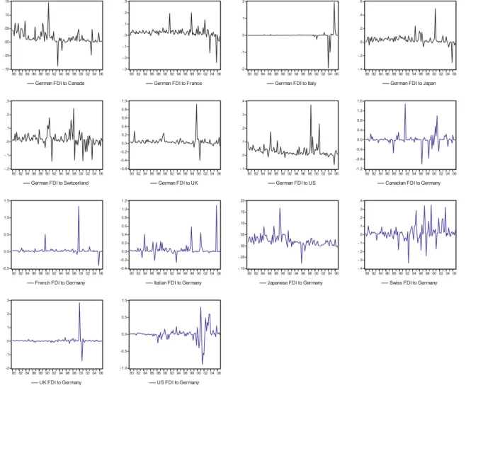
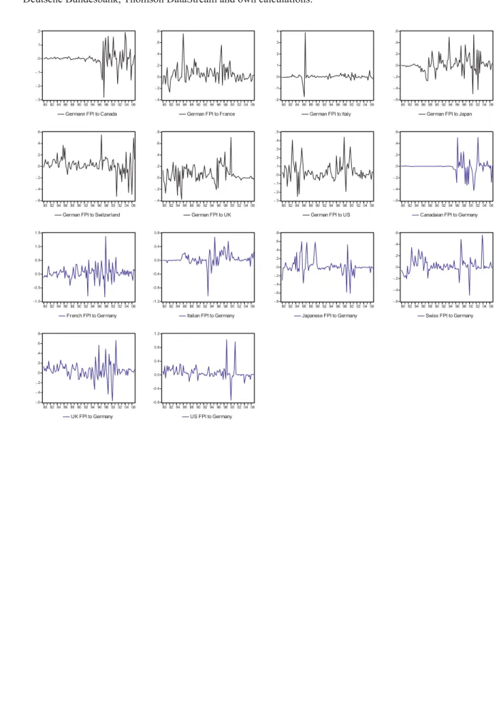
The continuously compounded quarterly growth rates of the stock of FDI and the stock of FPI are calculated in Deutschmark from 1980 until the end of 1998 and in Euro from 1999 until fourth quarter of 2006, with a sample size of 108 observations. The time-series characteristics of the growth rates of the stock of equity FDI and equity FPI, respectively, are summarized in Figure 1 and Figure 2.

The main observations are that (1) the growth rates of the stock of capital, whether FDI or FPI, are highly volatile, (2) all time-series show several extreme outliers, and (3) that our data are stationary.

[Insert Figures 1-2, here]

We also collect data from Thomson DataStream (DS): the total return, the market capitalization, and market-to-book (our proxy for Tobin’s q) on the DS country indexes in our data and on the DS World Index. From this raw data we construct continuously compounded quarterly returns. We also collect exchange rates as to convert all data into Deutschmark prior 1999 and into Euro thereafter. Again the sample size is 108 observations16.

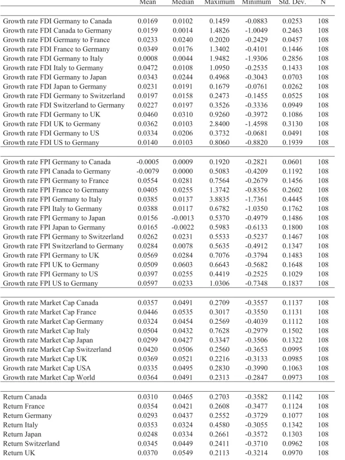
[Insert Table 1, here]

Table 1 reports basic descriptive statistics (mean, median, maximum, minimum, standard deviation, and the number of observations) for capital flow growth rates and for the independent variables employed in this study. The independent variables are Tobin’s q, the relative foreign equity return, home equity return, resources (human capital, technology, and the production relevant information set available abroad), and lagged growth rates and stock of the foreign capital.

16

The DS time series for the Tobin’s q variable for Canada (80), France (96), Italy (84), and Switzerland (84) is available only after 1980.

We construct these variables as follows. The growth rate of the market capitalization is the continuously compounded change in market capitalization. The relative foreign equity return is the rate of growth in host country market capitalization minus the rate of growth in the world market capitalization. Tobin’s q is the domestic market-to-book ratio. The variable “Resources” is the residuals of the long run relation between the market capitalization abroad and that in the rest of the world. It aims at measuring the discounted specific assets available in the host country.

In order to save space we do not report correlations for the data employed in the FDI and FPI models. We, however, remark that the correlations are small overall in both models. Therefore, the correlation coefficients do not suggest that our empirical regressions are spurious. Importantly, many correlation coefficients between the growth rate of FDI and Tobin’s q show negative sign. So, our results below are not a mere consequence of data that happen to move together over time.

It remains to remark that pair wise correlations of FDI and FPI from one country to another are mostly negative and small. Thus, none of the correlation coefficient suggests a mechanical relation between pair wise FDI and FPI. The tables with correlations are available upon request.

4. Empirical Results

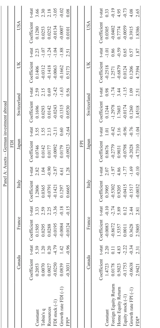
In Table 2, we present coefficient estimates and robust (HAC) GMM t-statistics of 2SLS simultaneous foreign direct investment (FDI) flow models and foreign portfolio investment (FPI) flow models. Panel A contains estimates of German investment abroad (asset side). Panel B contains estimates of foreign investment in Germany (liability side).

Tobin’s q, resources, lagged stock of equity FDI, lagged growth rate of the stock of equity FDI, and fitted FPI from the first stage regression are employed to explain the growth

rate of the stock of equity FDI. Relative foreign equity return, home equity return, lagged stock of equity FPI, lagged growth rate of the stock of equity FPI, and fitted FDI from the first stage regression explain the growth rate of the stock of equity portfolio investment.

As for German FDI, we find that our predictions are generally robust. More specifically, the Tobin’s q variable shows with the exception of UK the predicted sign. However, statistical significance is not always achieved. Essentially, the same can be said about Resources.

The FPI model performs also well. In particular, the Home Equity Return variable is estimated as predicted and with large statistical significance, except for UK. Both lagged variables, the stock of FPI and the growth rate of FPI, also provide explanatory power, but less consistently. Relative foreign equity return yields significant results with positive and negative coefficient estimates. As predicted, assets are influenced mostly negatively by relative foreign equity return while liabilities are positively influence. The negative coefficients arise because relative foreign equity return variable picks up wealth effects.

When it comes to simultaneity we find little evidence for FPI to impact FDI. To the contrary, FDI explains FPI investment. The coefficient estimates for the fitted FDI variable from the first stage regressions in the FPI regression in Table 2 (Panel A) are large, positive and highly significant, except for Italy and Japan. Overall, we find that the regressions for Canada, France, Switzerland, the UK and the USA strongly support our models. The empirical evidence for Japan is somewhat inconsistent, as a negative and significant coefficient for FPI in the FDI model is not easy to interpret. It is remarkable that the Japanese economy did not grow in real terms in the years 1991–2002. Furthermore, since 1994 Japan has experienced deflation of about 1%–2% a year despite the Bank of Japan’s “Zero Interest

Rate” policy. The consequences of the Japan’s stock and real estate market bubble burst in 1989, which lasted more than a decade, might also be behind such inconsistency.17

On the liability side, Panel B, the results are somewhat weaker. On the one hand, Tobin’s q and Home Equity Return still perform quite well. On the other hand, Tobin’s q is insignificant in the regression for the US and so is the fitted FDI in the FPI regression. Similarly, the coefficient estimates for the fitted FDI variable from the first stage regressions in the FPI regression in Table 2 (Panel B) are large and positive. However, they are highly significant only in the case of Canada, Japan and the UK.

It is common knowledge that collecting data from foreign multinational enterprises and from foreign portfolio mangers is much more difficult for statistical offices. Therefore, these results and particularly the evidence on the asset side are supportive of the predictions of this paper.

[Insert Table 2, here]

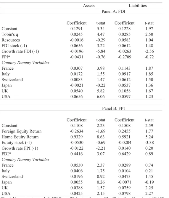
Table 3 shows coefficient estimates and robust (HAC) GMM t-statistics of pooled 2SLS simultaneous FDI and FPI flow models. The columns two and three show the regression estimates for German investment abroad, while columns four and five contain estimates for foreign investment in Germany. Tobin’s q is highly significant and shows the predicted sign for both assets and liabilities. The resources variable and the fitted FPI variables is always insignificant.

In the FPI regression, relative foreign equity return switches sign from asset side to liability side. Both coefficients are slightly insignificant. We again want to stress that the data on liabilities is potentially of very different quality. The coefficients estimates for the Home Equity Return are quite large, positive and highly significant. Last but not least, the fitted FDI

17

variable from the first stage regression is estimated with positive sign for both assets and liabilities. Again only the coefficient on the asset side is strongly statistically significant.

All in all, since FDI and FPI transactions are extremely volatile we believe that results presented above and, in particular, the effect of FDI decisions on international portfolio allocation, are an accomplishment. As a rule of thumb, we find that a 1% increase in the expected growth rate of FDI raises the growth rate of FPI by 0.5%.

[Insert Table 3, here]

5. Robustness Checks

We have conducted a battery of robustness checks by controlling for additional potential variables, such as stock and exchange rate volatility, or by considering alternative instruments. To save space we do not include all the corresponding tables, but they are available upon request. Further, we comment only on the two most obvious concerns. First, because the simultaneous regressions suggest that there is no simultaneity between FDI and FPI, the presented regressions for the FDI models could be misspecified. Simple OLS regressions, however, suggest that the coefficient estimates of the variables from the FDI models are robust to the inclusion of the fitted FPI variables.

Second, we also run OLS regressions with the actual FDI data instead of the fitted data in the FPI regressions, but do not find that FDI helps to explain FPI. Indirectly, we obtain additional supportive evidence for our FDI model, which is the model that investors are not only aware of, but also employ for portfolio investment purposes.

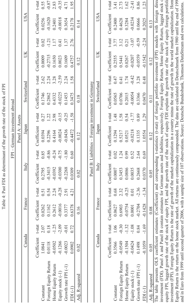
Third, we run OLS regressions with the actual past FDI data (see Table 4). Results are very weak on the liability side with several coefficient estimates showing a negative sign. On the asset side, we obtain again the positive coefficients, which however are only statistically

significant for France, the UK and the US. Consistently with previous findings, past FDI transactions do not help explaining FPI decisions.

6. Conclusions

This paper contributes to the growing literature on foreign direct investment (FDI) and to the growing literature on foreign portfolio investment (FPI). Unlike many other studies we analyze the interlinkages between FDI and FPI transactions between Germany and the major economies. One important contribution of our paper is that we address the joint dynamics of FDI and FPI, making use of a data set from Deutsche Bundesbank that has not received much attention.

We focus on two central research questions: What is the common driving force of FDI and FPI flows? Are there any informational linkages between FDI and FPI which would justify the joint dynamics?

The evidence put forward above lends support to the argument that that the most important factor determining equity capital flows is the stock market. First, we show that Tobin’s q helps explaining the variation of the growth rate of the stock of FDI. Second, we show that relative foreign equity return and home stock market return explain the variation of the growth rate of the stock of FPI.

Most importantly, we find that information about foreign fundamentals is revealed via direct investment. In other words, FDI transactions measured by fitted growth rates of the stock of FDI help explaining current growth rates of the stock of FPI. Conversely, actual and past FDI growth rate do not help explaining FPI transactions. To our knowledge this observation is the first unambiguous evidence that international portfolio investors follow firms’ expected foreign investment decisions.

Finally, we do not detect any evidence for the argument that swift portfolio investors are the first to spot foreign investment opportunities. If there is any simultaneous link between equity FDI and equity FPI flows, we could not find it in the data.

References

Albuquerque, R., Bauer, G.H. and M. Schneider, 2006a, International Equity Flows and Returns: A quantitative Equilibrium Approach, forthcoming Review of Economic Studies. Albuquerque, R., Bauer, G.H. and M. Schneider, 2006b, Global Private Information in

International Equity Markets, Working Paper.

Anderson, E. W., Ghysels, E. and J. L. Juergens, (2005), Do Heterogeneous Beliefs Matter for Asset Pricing?, Review of Financial Studies 18, 875-924.

Basak, S., 2000, A Model of Dynamic Equilibrium Asset Pricing with Heterogeneous Beliefs and Extraneous Risk, Journal of Economic Dynamics and Control 24, 63-95.

Blonigen, B.A., 1997, Firm-Specific Assets and the Link between Exchange Rates and Foreign Direct Investment, American Economic Review 87, 447-465.

Bond, S. and J. Cummins, 2001, Noisy Share Prices and the q Model of Investment, IFS Working Paper, WP01/22.

Brennan, M.J. and H.H. Cao, 1997, International Portfolio Investment Flows, Journal of Finance 52, 1851-1880.

Brennan, M.J., Cao, H.H., Strong, N. and X. Xu, 2005, The Dynamics of International Equity Market Expectations, Journal of Financial Economics 77, 257-288.

Chan, Y.L. and L. Kogan, 2002, Catching Up with the Joneses: Heterogeneous Preferences and the Dynamics of Asset Prices, Journal of Political Economy 110, 1255-1285.

Constantinides, G.M. and D. Duffie, 1996, Asset Pricing with Heterogeneous Consumers, Journal of Political Economy 104, 219-240.

De Santis, R.A. and F. Stähler, 2004, Endogenous Market Structures and the Gains from Foreign Direct Investment, Journal of International Economics 64, 545-565.

De Santis, R.A., Anderton R. and A. Hijzen, 1995, On the Determinants of Euro Area FDI to the United States: The Knowledge-Capital-Tobin’s q Framework, ECB Working Paper Series, NO. 329.

Detemple, J.B. and S. Murthy, 1994, Intertemporal Asset Pricing with Heterogeneous Beliefs, Journal of Economic Theory 62, 294-320.

Detemple, J.B., Garcia, R. and M. Rindisbacher, 2003, A Monte Carlo Method for Optimal Portfolios, Journal of Finance 58, 401-446.

Dumas, B., 1989, Two-Person Dynamic Equilibrium in the Capital Market, The Review of Financial Studies 2, 157-188.

Erickson, T. and T.M. Whited, 2000, Measurement Error and the Relationship between Investment and q, Journal of Political Economy 108, 1027-1057.

Forbes, K.J. and R. Rigobon, 2002, No Contagion, Only Interdependence: Measuring Stock Market Comovements, Journal of Finance 57, 2223-2261.

French, K. and J. Poterba, 1991, Investor Diversification and International Equity Markets, American Economic Review 81, 222-226.

Froot, K.A., O’Conell, P.G.J. and M.S. Seasholes, 2001, The Portfolio Flows of International Investors, Journal of Financial Economics 59, 151-193.

Goldstein, I., and A. Razin, 2006, An Information-Based Trade Off between Foreign Direct Investment and Foreign Portfolio Investment, Journal of International Economics 70. 271-295.

Griffin, J.M., Nardari, F., and R.M. Stulz, 2004, Are Daily Cross-Border Equity Flows Pushed or Pulled?, Review of Economics and Statistics 86, 641-657.

Hamao, Y., Mei, J. and Y. Xu, 2007, Unique Symptoms of Japanese Stagnation: An Equity Market Perspective, Journal of Money, Credit and Banking, 39, 901-923.

Hayashi, F., 1982, Tobin's Marginal q and Average q: A Neoclassical Interpretation, Econometrica, 50, 213-224.

Jovanovic, B. and P.L. Rouseau, 2002, The q-Theory of Mergers, American Economic Review 92, 198-204.

Lipster, R. and A. Shiryayev, 2001, Statistics and Random Processes II: Applications, Springer Verlag, Berlin.

Markusen, J.R. and K.E. Maskus, 2001, General Equilibrium Approaches to the Multinational Firm: A Review of Theory and Evidence, in J. Harrigan (ed.), Handbook of International Trade, London: Basil Blackwell.

Markusen, J.R., 2002, Multinational Firms and the Theory of International Trade, Cambridge, The MIT Press.

Merton, R., 1969, Lifetime Portfolio Selection under Uncertainty: The Continuous Time Case, Review of Economics and Statistics 51, 247-257.

Moner-Colonques, R., Orts, V. and J.J. Sempere-Monerris, 2007, Asymmetric Demand Information and Foreign Direct Investment, Scandinavian Journal of Economics 109, 93-106.

Nualart, D., 1995, The Malliavin Calculus and Related Topics, Springer, Berlin.

Portes, R. and H. Rey, 2005, The determinants of Cross-Border Equity Flows, Journal of International Economics 65, 269-296.

Richards, A., 2005, Big Fish in Small Ponds: The Trading Behavior and Price Impact of Foreign Investors in Asian Emerging Equity Markets, Journal of Financial and quantitative Analysis 40, 1-27.

Stevens, G.V.G. and R.E. Lipsey, 1991, Interactions Between Domestic and Foreign Investment, Journal of International Money and Finance, 11, 40-62.

Wang, J., 1996, The Term Structure of Interest Rates in a Pure Exchange Economy with Heterogeneous Investors, Journal of Financial Economics 41, 75-110.

Williams, J.T., 1977, Capital Asset Prices with Heterogeneous Beliefs, Journal of Financial Economics 5, 219-239.

Zapatero, F., 1998, Effects of Financial Innovations on Market Volatility when Beliefs are Heterogeneous, Journal of Economic Dynamics and Control 22, 597-626.

Ziegler, A., 2002, State-Price Densities under Heterogeneous Beliefs, the Smile Effect, and Implied Risk Aversion, European Economic Review 46, 1539-1557.

7. Appendix A

In this appendix, we show the link between marginal q and average q. Multiply (5) by I_t, (6) by FDI_t and (7) by

k

t

. Then,

t t t t t t t FDI t t t I k hq k q FDI k FDI I k I ¸¸ ¹ · ¨¨ © § ¸¸ ¹ · ¨¨ © § G 1 G 1

t t t t t t t FDI F k t t I D k k r h qk qk k FDI G k I G » » ¼ º « « ¬ ª ¸¸ ¹ · ¨¨ © § ¸¸ ¹ · ¨¨ © § 2 2 ` 2 ` 2 G G . Since

t t

_{t t t t} k q k q dt k q d

_{, then using the latter two expressions}

» ¼ º « ¬ ª » ¼ º « ¬ ª t t FDI t t F k t t I t t D k t t t t k FDI FDI k G k I I k G k rq dt k q d 2 2 2 2 G G .

This differential equation can be solved as follows

rt t t FDI t t F k t t I t t D k t t Be k FDI FDI k G r k I I k G r k q _» ¼ º « ¬ ª » ¼ º « ¬ ª 2 2 2 1 2 1 G G .

The transversality condition implies that the last term approaches zero as t approaches infinity. If the production functions exhibit constant returns to scale, since D D_lD

t D t l G w and F l F F t F t l G w , then G_kDk_t GDw_tDl_tD and

¦

n j js js F t F t F t F k k G w l p a G 1 . Both these assumptions yield t t tk V q . (A1)

Therefore, (5) and (6) can be written as

¸¸ ¹ · ¨¨ © § 1 1 t t I t t k V k I G (A2) ¸¸ ¹ · ¨¨ © § 1 1 t t FDI t t k V k FDI G . (A3)

Expressions (A2) and (A3) should explain respectively the growth rates of domestic investment and FDI activities.

t t t FDI I t h k k V k _» ¼ º « ¬ ª ¸¸ ¹ · ¨¨ © § ¸ ¹ · ¨ © § 1 1 1 G G _{. (A4)}

Thus, the marginal adjustment cost model does not yield an “optimal capital” level but rather an optimal adjustment path.

8. Appendix B

In this Appendix we describe how the difference in beliefs about dividend growth evolves over time as well as state the propositions that are relevant for our purposes.

The relation between investors D’s and investors F’s, e.g. the domestic and foreign investor, state price densities is given by

Ft t Dt [K

K (B1)

where K denotes state price densities, domestic and foreign, and [ is the density process capturing the evolution of heterogeneity of beliefs over time. Its dynamics are described by the following equation

D t t t t dW d[ ' 7[ (B2)

where the difference in beliefs process, ', is given by

Dt Ft

t m m

' O7O 1/2 (B3)

whereO are volatility coefficients (containing both the domestic and foreign volatility coefficient) and m represent dividend growth rates as perceived by the investors. Again the perceived growth rates are two dimensional since both agents form beliefs about domestic and foreign dividend growth.

In the paper the state price density appears in the optimal portfolio polices in Equation (10) while the density process capturing the evolution of heterogeneity of beliefs appears in the sharing rule.

For equilibrium we require that the commodity market, the stock market, and the bond market are cleared. Now suppose that the economy is indeed in equilibrium, then, the following list of propositions is sufficient for existence of the optimal portfolio policy stated in Equations (10-11).

Proposition 1: When the economy is in equilibrium, then the state price density is given by

c t

u_{D Dt} Dt , ' K (B4)

where u denotes utility, (.)’ stands for first derivative of the utility function with respect to consumption and the second argument of the utility function is the time preference (E in Equation (9)).

Proposition 2: When the economy is in equilibrium, then wealth allocations are given by

»_¼ º « ¬ ª

³

f t is Ds D Dt Dt D it E u c s c ds t c u X , , 1 ' ' (B5)

where i

D,F

denote domestic and foreign, respectively.

Proposition 3: When the economy is in equilibrium, then optimal portfolio polices are given by

Dt t Dt

>

t i

@

Dt t it it X V T K V E \ H I , 1 1 1 7 (B6) where

³

f 0 ' ,t c dt c u H_{i D Dt it} . (B7)

Finally, the Malliavin derivative of H_i, e.g. \_tH_i, is given by Equation (11).

To save space we do not state the propositions for the endogenous equilibrium covariance matrix of stock returns, V , and the Sharpe ratio, T. These propositions as well as the proofs are available upon request.

9. Appendix C

In this Appendix we describe how to filter two (dependent or independent) processes. Consider the following system

» ¼ º « ¬ ª » ¼ º « ¬ ª » ¼ º « ¬ ª » ¼ º « ¬ ª t t t t t t t dW dW dt x x dy dy dy 2 1 22 21 12 11 2 1 2 1 V V V V (C1)

where V is known and x is unknown. In order to simplify the exposition assume that x is a constant. The problem is to estimate x based on the observation of y. The Kalman-Bucy filter is used to solve this problem. Assume that at time t=0 the prior of x is normal with mean m0 and variance V 0 . As time passes by the prior is updated via y.

The mean of y is updated according to (Lipster and Shiryayev, 2001):

t t t V dW dm VV7 1/2 ~ (C2) where

dy mdt

W d ~_t VV7 1/2 _{t t} . (C3)

The variance of the mean is updated as follows

V dt

V

dV_{t t} VV7 1/2 _t T . (C4)

Under such general dependency between two processes (in our model FDI and dividends or output) one cannot learn about the mean of one process without learning also the mean of the second moment even when it is unnecessary. In the language of our model this means portfolio investors must learn from FDI in order to estimate dividend (or output) growth.

Even when the processes follow somewhat simpler dynamics it can be beneficial to learn from two processes. Consider the following setting:

» ¼ º « ¬ ª » ¼ º « ¬ ª » ¼ º « ¬ ª » ¼ º « ¬ ª t t t t t dW dW dt x x dy dy dy 2 1 22 11 2 1 0 0 V V . (C5)

Although here one can filter (learn) about the growth rate of the first process independently of the second process and may, thus, disregard the second process. However, m_t m_1tm_2t will converge faster and with lower variance to x than m1t or m2t. Therefore, it is suboptimal to

ignore a second process growing with the same rate. Again in the language of our model this means even if FDI growth would not directly impact dividend growth (consumption or GDP growth) portfolio investors may nevertheless find it optimal to use it to estimate dividend growth as long as it helps to increase the speed of learning, decrease the noise in estimates, or both.

Figures

Figure 1. This figure displays the growth rate of the stock of FDI. The data are calculated in Deutschmark from 1980 until the end of 1998 and in Euro from 1999 until second quarter of 2006, with a sample size of 106 observations. The stocks of FDI are calculated with quarterly data starting with the first quarter in 1971. Sources: Deutsche Bundesbank, Thomson DataStream and own calculations.

-.10 -.05 .00 .05 .10 .15 80 82 84 86 88 90 92 94 96 98 00 02 04 06

German FDI to Canada

-.3 -.2 -.1 .0 .1 .2 .3 80 82 84 86 88 90 92 94 96 98 00 02 04 06

German FDI to France

-2 -1 0 1 2 80 82 84 86 88 90 92 94 96 98 00 02 04 06

German FDI to Italy

-.4 -.2 .0 .2 .4 .6 80 82 84 86 88 90 92 94 96 98 00 02 04 06

German FDI to Japan

-.2 -.1 .0 .1 .2 .3 80 82 84 86 88 90 92 94 96 98 00 02 04 06

German FDI to Switzerland

-0.6 -0.4 -0.2 0.0 0.2 0.4 0.6 0.8 1.0 80 82 84 86 88 90 92 94 96 98 00 02 04 06 German FDI to UK -.1 .0 .1 .2 .3 .4 80 82 84 86 88 90 92 94 96 98 00 02 04 06 German FDI to US -1.2 -0.8 -0.4 0.0 0.4 0.8 1.2 1.6 80 82 84 86 88 90 92 94 96 98 00 02 04 06

Canadian FDI to Germany

-0.5 0.0 0.5 1.0 1.5 80 82 84 86 88 90 92 94 96 98 00 02 04 06

French FDI to Germany

-0.4 -0.2 0.0 0.2 0.4 0.6 0.8 1.0 1.2 80 82 84 86 88 90 92 94 96 98 00 02 04 06

Italian FDI to Germany

-.10 -.05 .00 .05 .10 .15 .20 80 82 84 86 88 90 92 94 96 98 00 02 04 06

Japanese FDI to Germany

-.4 -.3 -.2 -.1 .0 .1 .2 .3 .4 80 82 84 86 88 90 92 94 96 98 00 02 04 06

Swiss FDI to Germany

-2 -1 0 1 2 3 80 82 84 86 88 90 92 94 96 98 00 02 04 06 UK FDI to Germany -1.0 -0.5 0.0 0.5 1.0 80 82 84 86 88 90 92 94 96 98 00 02 04 06 US FDI to Germany

Figure 2. This figure displays the growth rate of the stock of FPI. The data are calculated in Deutschmark from 1980 until the end of 1998 and in Euro from 1999 until second quarter of 2006, with a sample size of 106 observations. The stocks of FPI are calculated with quarterly data starting with the first quarter in 1971. Sources: Deutsche Bundesbank, Thomson DataStream and own calculations.

-.3 -.2 -.1 .0 .1 .2 80 82 84 86 88 90 92 94 96 98 00 02 04 06

Germann FPI to Canada

-.4 -.2 .0 .2 .4 .6 .8 80 82 84 86 88 90 92 94 96 98 00 02 04 06

German FPI to France

-2 -1 0 1 2 3 4 80 82 84 86 88 90 92 94 96 98 00 02 04 06

German FPI to Italy

-.6 -.4 -.2 .0 .2 .4 .6 80 82 84 86 88 90 92 94 96 98 00 02 04 06

German FPI to Japan

-.6 -.4 -.2 .0 .2 .4 .6 80 82 84 86 88 90 92 94 96 98 00 02 04 06

German FPI to Switzerland

-.4 -.2 .0 .2 .4 .6 .8 80 82 84 86 88 90 92 94 96 98 00 02 04 06 German FPI to UK -.3 -.2 -.1 .0 .1 .2 .3 .4 .5 80 82 84 86 88 90 92 94 96 98 00 02 04 06 German FPI to US -.6 -.4 -.2 .0 .2 .4 .6 80 82 84 86 88 90 92 94 96 98 00 02 04 06

Canadaian FPI to Germany

-1.0 -0.5 0.0 0.5 1.0 1.5 80 82 84 86 88 90 92 94 96 98 00 02 04 06

French FPI to Germany

-1.2 -0.8 -0.4 0.0 0.4 0.8 80 82 84 86 88 90 92 94 96 98 00 02 04 06

Italian FPI to Germany

-.8 -.6 -.4 -.2 .0 .2 .4 .6 .8 80 82 84 86 88 90 92 94 96 98 00 02 04 06

Japanese FPI to Germany

-.6 -.4 -.2 .0 .2 .4 .6 80 82 84 86 88 90 92 94 96 98 00 02 04 06

Swiss FPI to Germany

-.6 -.4 -.2 .0 .2 .4 .6 .8 80 82 84 86 88 90 92 94 96 98 00 02 04 06 UK FPI to Germany -0.8 -0.4 0.0 0.4 0.8 1.2 80 82 84 86 88 90 92 94 96 98 00 02 04 06 US FPI to Germany