remote sensing
ArticleEnhanced Feature Extraction for Ship Detection from
Multi-Resolution and Multi-Scene Synthetic Aperture
Radar (SAR) Images
Fei Gao1 , Wei Shi1 , Jun Wang1,*, Erfu Yang2and Huiyu Zhou3
1 Electronic Information Engineering, Beihang University, Beijing 100191, China; 08060@buaa.edu.cn (F.G.); sw1995@buaa.edu.cn (W.S.)
2 Space Mechatronic Systems Technology Laboratory, Department of Design, Manufacture and Engineering, Management, University of Strathclyde, Glasgow G11XJ, UK; erfu.yang@strath.ac.uk
3 Department of Informatics, University of Leicester, Leicester LE1 7RH, UK; hz143@leicester.ac.uk * Correspondence: wangj203@buaa.edu.cn; Tel.:+86-135-8178-4500
Received: 1 October 2019; Accepted: 15 November 2019; Published: 18 November 2019 Abstract:Independent of daylight and weather conditions, synthetic aperture radar (SAR) images have been widely used for ship monitoring. The traditional methods for SAR ship detection are highly dependent on the statistical models of sea clutter or some predefined thresholds, and generally require a multi-step operation, which results in time-consuming and less robust ship detection. Recently, deep learning algorithms have found wide applications in ship detection from SAR images. However, due to the multi-resolution imaging mode and complex background, it is hard for the network to extract representative SAR target features, which limits the ship detection performance. In order to enhance the feature extraction ability of the network, three improvement techniques have been developed. Firstly, multi-level sparse optimization of SAR image is carried out to handle clutters and sidelobes so as to enhance the discrimination of the features of SAR images. Secondly, we hereby propose a novel split convolution block (SCB) to enhance the feature representation of small targets, which divides the SAR images into smaller sub-images as the input of the network. Finally, a spatial attention block (SAB) is embedded in the feature pyramid network (FPN) to reduce the loss of spatial information, during the dimensionality reduction process. In this paper, experiments on the multi-resolution SAR images of GaoFen-3 and Sentinel-1 under complex backgrounds are carried out and the results verify the effectiveness of SCB and SAB. The comparison results also show that the proposed method is superior to several state-of-the-art object detection algorithms.
Keywords: Ship Detection; Feature Enhancement; Split Convolution Block (SCB); Spatial Attention Block (SAB)
1. Introduction
Due to the all-weather, all-day characteristics, SAR has become one of the important means of earth observation [1], such as vehicle detection [2], river detection [3] and image recognition [4,5]. Through airborne and spaceborne SAR, a large number of high resolution SAR ocean images can be obtained. Ship detection from SAR images is one of the important research directions of SAR image interpretation, and is widely used in military and civilian fields. The traditional method for ship detection from SAR images includes statistical distribution-based methods [6–9], multi-scale-based methods [10], template matching [11] and multiple/full polarization-based methods [12,13]. These methods highly rely on the distributions of sea clutters and the predefined thresholds [14–16]. At the same time, traditional ship detection systems usually consist of several steps, including land masking, preprocessing, prescreening and discrimination [17,18]. The multi-step operation mode of the traditional methods leads to
Remote Sens.2019,11, 2694 2 of 22
time-consuming and low robustness of detection. Deep learning has also been applied to SAR ship detection [19–25].
The object detection algorithm based on deep learning has surpassed the traditional detection methods and become very popular with the merits of no need for feature extraction by hand, good feature expression ability and high detection accuracy. Object detection algorithms based on deep learning mainly include one-stage and two-stage detectors. The one-stage detectors directly convert the target detection into a regression problem which is fast running. In the two-stage detectors, the first stage generates a sparse set of candidate proposals that contain all the objects while filtering out the majority of negative locations, and the second stage classifies the proposals into foreground/background. The two-stage detectors achieve higher accuracy with low efficiency.
In terms of one-stage detectors, Wang et al. [20] apply the end-to-end RetinaNet to SAR ship detection, construct a multi-resolution and complex background dataset and achieve high detection accuracy. In order to reduce computational time with relatively competitive detection accuracy, Chang et al. [21] develop a new architecture with less number of layers called YOLOv2-reduced. With respect to two-stage detectors, Hu et al. [22] use Faster-RCNN to detect SAR ships under the multi-resolution condition. They design the convolution neural network (CNN) architecture based on the characteristics of sea clutter with different resolutions through SAR simulation, and achieve good detection performance on the high resolution TerraSAR-X and low-resolution sentinel-1 SAR datasets. Zhao et al. [23] develop a coupled CNN for small and densely cluttered SAR ship detection, which is better than the traditional CFAR detection algorithm in detection accuracy and time consumption. Considering the difference between each layer, both of these detectors at multi-scales usually use feature maps of different layers for prediction.
The shallow layers of CNNs collect the detailed features of the image, which is convenient for detecting small targets. The high-levels of the network extract the abstract features of the input image, which is convenient for detecting large targets [26]. However, due to the limited parameters of the shallow layers, the low resolution and few features of small targets, it is difficult to extract features by the standard CNNs. Especially for densely clustered small targets, the standard multi-scale target detection algorithms still cannot achieve good results, so the feature extraction ability of the network needs to be enhanced.
To enhance the performance of CNNs, researchers have mainly investigated three important factors of the network: depth [27], width [28–30] and cardinality [31]. These measures will improve the nonlinearity of the network and enhance the feature representation ability, but it will not help the feature extraction of small targets, and will make the network too large and difficult to train. During the feature extraction of CNNs, the convolution kernels are globally optimized on the entire input image. Due to the overall priority in visual information processing, it is easy to lose the details of the small targets. In order to enhance the details of small targets, a standard method is to interpolate and zoom the small targets [32]. However, the interpolation of a SAR image will damage the original features of the SAR image and destroy the ground resolution [33,34]. Aiming at the small SAR targets detection in complex backgrounds, we propose a new convolution block, namely the split convolution block (SCB). SCB divides the SAR images into smaller sub-images as input to the network, and then fuses the feature maps obtained from the sub-images to achieve feature extraction on a finer granularity. As a result, the network will pay more attention to the details of targets in addition to the global features. With the help of SCB, the proportion of small targets in each sub-image will be expanded, and the difficulty of feature extraction of small targets will be reduced, so as to avoid neglecting the detailed features caused by the overall priority. Apart from SCB, we still retain a normal convolution path, take the whole SAR image without split as the input, and keep the global features of the input image. After the first convolution module, the result of SCB is fused with the result of normal convolution to obtain the feature map that is emphasized so as to realize feature extraction enhancement.
The correctness of the SAR image interpretation is closely related to the SAR image quality. For the purpose of SAR image feature enhancement, we perform sparse optimization on SAR images to
Remote Sens.2019,11, 2694 3 of 22
achieve clutters and sidelobes suppression in the preprocessing stage [35,36]. The baseline model used in this paper is RetinaNet [37], which embeds FPN [26] as the backbone. The FPN feedforward network transmits the feature map to the feature pyramid net, and uses 1×1 convolution for the feature dimensionality reduction. In order to reduce the loss of spatial information during feature dimensionality reduction, we add the spatial attention block (SAB) to enhance the spatial features. SAB greatly improve the efficiency and accuracy of spatial information processing. The proposed method achieves high detection accuracy on the multi-resolution and multi-scene GaoFen-3 [38] and Sentinel-1 [39] images, realizing the accurate positioning of targets with a low false alarm rate.
The rest of this paper is arranged as follows. Section2describes the proposed method in detail, including the background of RetinaNet, SCB and SAB. Our experiments and results are presented in Section3. Finally, we summarize this paper in Section4.
2. Materials and Methods
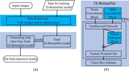
The overall scheme of the proposed method and the network architecture of 2S-RetinaNet (Split Convolution and Spatial Attention Blocks-RetinaNet) are shown in Figure1. As shown in Figure1a, before sending the SAR images into the network, we perform the sparse optimization on the input SAR images to achieve clutter and sidelobe suppression, and improve the signal to clutter ratio of the image. Due to the SAR image quality in the dataset, the sparse optimization is carried at muti-levels. On the basis of RetinaNet, two self-designed modules, namely SCB and SAB are embedded. The locations of these two modules in the overall network are shown in Figure1b. SCB divides the input SAR images into smaller parts to improve the attention to small and densely clustered ships. And SAB optimizes the feature maps of the FPN feedforward network, strengthens the attention to the target area, and reduces the loss of spatial information during the feature maps transfer between the feedforward network and the feature pyramid net. After that, the box and class regression subnets will predict the target position and classification with the multi-layer feature maps extracted by FPN. The addition of SCB and SAB will not change the convergence of RetinaNet. At the same time, the increased running time is acceptable after the two lightweight modules embedded.
Remote Sens. 2019, 11, x FOR PEER REVIEW 3 of 23
achieve clutters and sidelobes suppression in the preprocessing stage [35,36]. The baseline model used in this paper is RetinaNet [37], which embeds FPN [26] as the backbone. The FPN feedforward network transmits the feature map to the feature pyramid net, and uses 1 × 1 convolution for the feature dimensionality reduction. In order to reduce the loss of spatial information during feature dimensionality reduction, we add the spatial attention block (SAB) to enhance the spatial features. SAB greatly improve the efficiency and accuracy of spatial information processing. The proposed method achieves high detection accuracy on the multi-resolution and multi-scene GaoFen-3[38] and Sentinel-1[39] images, realizing the accurate positioning of targets with a low false alarm rate.
The rest of this paper is arranged as follows. Section II describes the proposed method in detail, including the background of RetinaNet, SCB and SAB. Our experiments and results are presented in Section III. Finally, we summarize this paper in Section IV.
2. Materials and Methods
The overall scheme of the proposed method and the network architecture of 2S-RetinaNet (Split Convolution and Spatial Attention Blocks-RetinaNet) are shown in Figure 1. As shown in Figure 1a, before sending the SAR images into the network, we perform the sparse optimization on the input SAR images to achieve clutter and sidelobe suppression, and improve the signal to clutter ratio of the image. Due to the SAR image quality in the dataset, the sparse optimization is carried at muti-levels. On the basis of RetinaNet, two self-designed modules, namely SCB and SAB are embedded. The locations of these two modules in the overall network are shown in Figure 1b. SCB divides the input SAR images into smaller parts to improve the attention to small and densely clustered ships. And SAB optimizes the feature maps of the FPN feedforward network, strengthens the attention to the target area, and reduces the loss of spatial information during the feature maps transfer between the feedforward network and the feature pyramid net. After that, the box and class regression subnets will predict the target position and classification with the multi-layer feature maps extracted by FPN. The addition of SCB and SAB will not change the convergence of RetinaNet. At the same time, the increased running time is acceptable after the two lightweight modules embedded.
Figure 1. (a): The overall framework of the proposed method; (b): The architecture of 2S-RetinaNet.
In addition, based on the distribution of the bounding box in the dataset, we re-design the structure of RetinaNet and the size of the anchor of each layer in FPN. In the following sections, the SAR image sparse optimization, the background on RetinaNet and the three improvements on RetineNet: multi-scale anchor design, SCB and SAB, are presented.
2.1. Data Preprocess: SAR Image Sparse Optimization
Figure 1.(a): The overall framework of the proposed method; (b): The architecture of 2S-RetinaNet. In addition, based on the distribution of the bounding box in the dataset, we re-design the structure of RetinaNet and the size of the anchor of each layer in FPN. In the following sections, the SAR image sparse optimization, the background on RetinaNet and the three improvements on RetineNet: multi-scale anchor design, SCB and SAB, are presented.
Remote Sens.2019,11, 2694 4 of 22
2.1. Data Preprocess: SAR Image Sparse Optimization
For space-borne SAR systems, the radar receives echo signals from the ground, including ground-based stationary clutter and moving target signals. Since the spectrum of the clutter is wide and the energy of the clutter is much stronger than the energy of the target, we need to suppress the clutters to improve the target detection ability. In the multi-targets SAR images, the high-level sidelobes of the strong scattering point will mask the low-level main lobe of the adjacent weak scatter target, resulting in the missed detection of the weak targets. Due to the metal materials and the superstructure of the ship, ships have strong backscatters. Generally, the metallic ship cockpits produce bright lines along the range or the azimuth directions which are caused by the sidelobe effect. These bright lines will reshape the ship appearances in the SAR images and disturb the detection process.
In this paper, we perform sparse optimization via an iterative thresholding algorithm to enhance the features of the SAR image at first. Compared with the traditional SAR feature enhancement methods, it can achieve the performance improvement in clutter, sidelobe and azimuth ambiguity suppression, with additional advantage of lower computational complexity and memory consumption. As for a SAR image obtained by radar system, it can be decomposed as follows:
Y=X+N (1)
whereXis the considered scene. Nis a complex matrix of the same size asX, which denotes the difference between reconstructed image and the real scene, and includes noise, sidelobe, clutter, azimuth ambiguity and so on. Considering the sparsity of SAR images, we can recover the considered scene by solving the following optimization problem:
ˆ X=min X n kY−Xk2 F+λkXk q q o (2) Here, we takeLqregularization-based synthetic aperture radar image feature enhancement, and q∈(0, 1]. Where ˆXis theLqregularization-based reconstructed scene,λis the regularization parameter andk•k
Fis the Fresenius norm of a matrix. An iterative thresholding algorithm is often used to solve the optimization problem [40]. Whenq=1, the detailed approximated sequence of the solution can be represented as:
X(i+1)= f(X(i)+µ(Y−X(i)),µλ) (3) whereX(i) is the reconstruction scene of theith iteration and f(.)is the thresholding operator. µ controls the convergence speed of the iterative algorithm. The regularization parameterλcontrols the reconstructed precision and the estimated scene sparsity.λis updated after each iteration:
λ(i)= X (i)+µ∆X(i) K+1/µ (4)
where∆X(i)represents the difference between the reconstruction scene of the current iteration (X(i)) and the original image (Y). And
X
(i)+µ∆X(i)
K+1denotes the (K+1)st largest amplitude element of the image, whereKis a parameter denoting the scene sparsity, which can be obtained by calculating the zero norm of the reconstruction scene (X(i)):
K=∆ kX(i)k0/M (5)
where M is the number of the pixels ofX. Kandλare updated after each iteration, and the sparse reconstruction scene of the current iteration is:
X(i+1)=sgn(X(i)+µ∆X(i))·max( X
(i)+µ∆X(i)
Remote Sens.2019,11, 2694 5 of 22
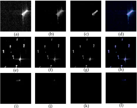
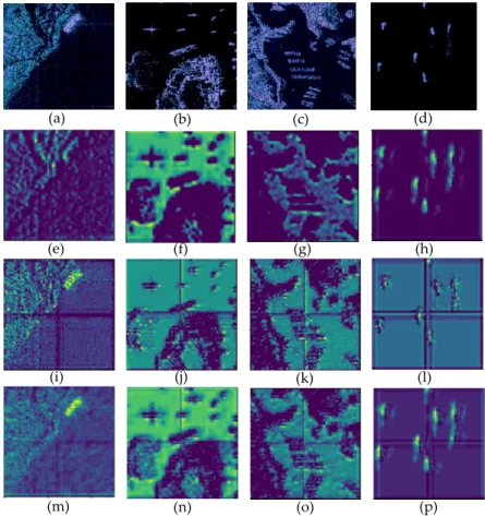
After multiple iterations, the signal values with lower amplitudes in the input scene will be set to zero to achieve clutter and sidelobe suppression. The number of the iteration has a great impact on the sparsity and precision of the reconstruction scene. Less iterations will retain more details in the original image, but at the same time the clutter and sidelobe suppression are not thorough enough. If the number of the iteration is set too high, the clutter and sidelobe will be better removed, but the details of the input image may be lost. As for the input SAR images with different quality, here we use the sparse reconstructed images under different iterations as the input of the network. In Figure2, three original SAR images are shown respectively, with iterations of 50 and 80, and three-channel RGB images that are fused with the original images and two sparse reconstruction images.
Remote Sens. 2019, 11, x FOR PEER REVIEW 5 of 23
After multiple iterations, the signal values with lower amplitudes in the input scene will be set to zero to achieve clutter and sidelobe suppression. The number of the iteration has a great impact on the sparsity and precision of the reconstruction scene. Less iterations will retain more details in the original image, but at the same time the clutter and sidelobe suppression are not thorough enough. If the number of the iteration is set too high, the clutter and sidelobe will be better removed, but the details of the input image may be lost. As for the input SAR images with different quality, here we use the sparse reconstructed images under different iterations as the input of the network. In Figure 2, three original SAR images are shown respectively, with iterations of 50 and 80, and three-channel RGB images that are fused with the original images and two sparse reconstruction images.
Figure 2. SAR images reconstructed by sparse optimization. (a), (b), (c) and (d) denote the original
image patch, the result of sparse optimization reconstruction with 50 iterations, the result of sparse optimization reconstruction with 80 iterations, the fusion result of the original image and the two of sparse optimization reconstruction results, respectively. (e), (f), (g) and (h) display the second image patch example and its corresponding results, respectively. (i), (j), (k) and (l) exhibit the third image patch example and its corresponding results, respectively.
As shown in Figure 2a–c, clutters and sidelobes in the SAR images are suppressed in the two dimensions of distance and azimuth, and the target becomes clearer with the increase of iterations. When the number of iterations is high, the non-target spots in the SAR image will be removed, which will reduce false alarms during the detection process. However, too many iterations will also cause the loss of the SAR target details. As shown in Figure 2j,k, some or all of the target features in SAR images are lost. SAR images with different quality need sparse optimization with different iterations. Therefore, we choose the original image, 50 and 80 iterations as the input of the network. As can be seen from Figure 2d,h,l, such a method enables the SAR images with different quality to be clutters and sidelobes suppressed without losing the original target features.
Deep learning networks are designed based on the optical images, and the input image has three input channels of RGB. For SAR grayscale images, there is only one input channel. In order to widely apply deep learning networks to SAR images, the common measure is to adopt the same grayscale image for all the three input channels. As a result, the features learned on these three channels will be overlapped. In this paper, the SAR original image and the image enhancement under two levels are taken as input, which enriches the characteristics of the SAR images and enables the network to learn more. (l) (k) (j) (h) (g) (f) (e) (d) (c) (b) (a) (i)
Figure 2.SAR images reconstructed by sparse optimization. (a), (b), (c) and (d) denote the original image patch, the result of sparse optimization reconstruction with 50 iterations, the result of sparse optimization reconstruction with 80 iterations, the fusion result of the original image and the two of sparse optimization reconstruction results, respectively. (e), (f), (g) and (h) display the second image patch example and its corresponding results, respectively. (i), (j), (k) and (l) exhibit the third image patch example and its corresponding results, respectively.
As shown in Figure2a–c, clutters and sidelobes in the SAR images are suppressed in the two dimensions of distance and azimuth, and the target becomes clearer with the increase of iterations. When the number of iterations is high, the non-target spots in the SAR image will be removed, which will reduce false alarms during the detection process. However, too many iterations will also cause the loss of the SAR target details. As shown in Figure2j,k, some or all of the target features in SAR images are lost. SAR images with different quality need sparse optimization with different iterations. Therefore, we choose the original image, 50 and 80 iterations as the input of the network. As can be seen from Figure2d,h,l, such a method enables the SAR images with different quality to be clutters and sidelobes suppressed without losing the original target features.
Deep learning networks are designed based on the optical images, and the input image has three input channels of RGB. For SAR grayscale images, there is only one input channel. In order to widely apply deep learning networks to SAR images, the common measure is to adopt the same grayscale image for all the three input channels. As a result, the features learned on these three channels will be overlapped. In this paper, the SAR original image and the image enhancement under two levels
Remote Sens.2019,11, 2694 6 of 22
are taken as input, which enriches the characteristics of the SAR images and enables the network to learn more.
2.2. Background on RetinaNet
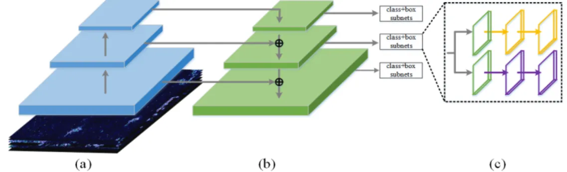
RetinaNet is a one-stage detector and mainly consists of a backbone network and two sub-networks. The network structure is shown in Figure3. Figure3a shows the bottom-up pathway for feature extraction, (b) shows the top-down pathway for feature fusion, (a) and (b) together form the backbone network FPN and (c) is the two subnetworks. FPN acts as a feature extractor with the consideration of the low-level high-resolution and high-level low-resolution semantic meaning. FPN mainly solves the multi-scale problem in object detection. By simply changing the network connection, the detection performance of small objects is greatly improved without substantially increasing of the calculation. The feedforward network of FPN usually consists of CNNs, such as VGG [27], Inception [28–30], ResNet [41,42] and DenseNet [43]. The two subnets are composed of the fully convolution network (FCN) [44]. One subnet is used for predicting the bounding box of the targets, and the other is used to predict the classification of the targets. Except for the final convolution layer, the design of the box regression subnet is identical to the classification subnet. The two subnets share a common structure but use separate parameters.
Remote Sens. 2019, 11, x FOR PEER REVIEW 6 of 23
2.2. Background on RetinaNet
RetinaNet is a one-stage detector and mainly consists of a backbone network and two sub-networks. The network structure is shown in Figure 3. Figure 3a shows the bottom-up pathway for feature extraction, (b) shows the top-down pathway for feature fusion, (a) and (b) together form the backbone network FPN and (c) is the two subnetworks. FPN acts as a feature extractor with the consideration of the low-level high-resolution and high-level low-resolution semantic meaning. FPN mainly solves the multi-scale problem in object detection. By simply changing the network connection, the detection performance of small objects is greatly improved without substantially increasing of the calculation. The feedforward network of FPN usually consists of CNNs, such as VGG [27], Inception [28–30], ResNet [41,42] and DenseNet [43]. The two subnets are composed of the fully convolution network (FCN) [44]. One subnet is used for predicting the bounding box of the targets, and the other is used to predict the classification of the targets. Except for the final convolution layer, the design of the box regression subnet is identical to the classification subnet. The two subnets share a common structure but use separate parameters.
Figure 3. The architecture of RetinaNet: The green parts are the pyramidal features extracted by
feature pyramid networks (FPN). The yellow and purple parts are the classification and the box regression subnets, respectively. (a) indicates the feedforward network. (b) is feature pyramid net to obtain the multi-scale features. (c) illustrates that there are two subnets, i.e., the top yellow one for classification and the purple bottom for bounding box regression.
In order to solve the problem of class imbalance in object detection, RetinaNet adopts focal loss as the loss function. Focal loss is an improved cross entropy loss, which multiplies an exponential term to weaken the contribution of easy examples. In Sections 2.2.1 and 2.2.2, we will introduce FPN and Focal loss in detail.
2.2.1. FPN (Feature Pyramid Network)
As shown in Figure 3, there are two pathways in FPN. The bottom-up pathway usually consists of CNNs to extract hierarchical features. The spatial resolution decreases from bottom to top, and semantic information in the feature maps increases as the network hierarchy is getting deeper.
The top-down pathway hallucinates higher resolution features by up-sampling spatially coarser, but semantically stronger, feature maps from higher pyramid levels. Then, these features are enhanced with the features from bottom-top pathway via lateral connections. The lateral connection merges the feature maps from the bottom-top and top-down pathways. The feature maps from the bottom-up pathway are of lower-level semantics, but more accurately localized as it is subsampled fewer times. As a result, the feature maps used for prediction features have different resolutions and semantic meanings. Such an operation only adds additional cross-layer connections on the basis of the original network, it hardly consumes extra time and computation.
To see more clearly, the architecture of FPN used in our method is presented in Figure.4. As shown in Figure 4, the input images used in this paper has a size of 256 × 256. After four convolution modules, the feature maps with a size of 32 × 32, 16 × 16, 8 × 8 {C2, C3, C4} are obtained, respectively. The skipped connections apply 1 × 1 convolution to reduce the channels of {C2, C3, C4} to 256. After
Figure 3.The architecture of RetinaNet: The green parts are the pyramidal features extracted by feature pyramid networks (FPN). The yellow and purple parts are the classification and the box regression subnets, respectively. (a) indicates the feedforward network. (b) is feature pyramid net to obtain the multi-scale features. (c) illustrates that there are two subnets, i.e., the top yellow one for classification and the purple bottom for bounding box regression.
In order to solve the problem of class imbalance in object detection, RetinaNet adopts focal loss as the loss function. Focal loss is an improved cross entropy loss, which multiplies an exponential term to weaken the contribution of easy examples. In Sections2.2.1and2.2.2, we will introduce FPN and Focal loss in detail.
2.2.1. FPN (Feature Pyramid Network)
As shown in Figure3, there are two pathways in FPN. The bottom-up pathway usually consists of CNNs to extract hierarchical features. The spatial resolution decreases from bottom to top, and semantic information in the feature maps increases as the network hierarchy is getting deeper.
The top-down pathway hallucinates higher resolution features by up-sampling spatially coarser, but semantically stronger, feature maps from higher pyramid levels. Then, these features are enhanced with the features from bottom-top pathway via lateral connections. The lateral connection merges the feature maps from the bottom-top and top-down pathways. The feature maps from the bottom-up pathway are of lower-level semantics, but more accurately localized as it is subsampled fewer times. As a result, the feature maps used for prediction features have different resolutions and semantic meanings. Such an operation only adds additional cross-layer connections on the basis of the original network, it hardly consumes extra time and computation.
Remote Sens.2019,11, 2694 7 of 22
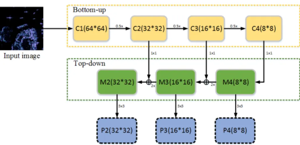
To see more clearly, the architecture of FPN used in our method is presented in Figure4. As shown in Figure4, the input images used in this paper has a size of 256 ×256. After four convolution modules, the feature maps with a size of 32×32, 16×16, 8×8 {C2, C3, C4} are obtained, respectively. The skipped connections apply 1×1 convolution to reduce the channels of {C2, C3, C4} to 256. After that, {M2, M3, M4} are obtained by combining the up-sampling feature maps with the corresponding bottom-up feature maps. Finally, a 3×3 convolution is used to obtain the feature maps for classification and bounding box regression. The final feature maps set is {P2, P3, P4}, with the same length and width as {C2, C3, C4}, respectively.
Remote Sens. 2019, 11, x FOR PEER REVIEW 7 of 23
that, {M2, M3, M4} are obtained by combining the up-sampling feature maps with the corresponding bottom-up feature maps. Finally, a 3 × 3 convolution is used to obtain the feature maps for classification and bounding box regression. The final feature maps set is {P2, P3, P4}, with the same length and width as {C2, C3, C4}, respectively.
Figure 4. The architecture of FPN: FPN: (i = 1, 2 … 4) is used to denote the convolutional block. The
skipped connections apply a 1 × 1 convolution filter to reduce the channels of Ci (i = 2, 3, 4) to 256. During the top-down flow, the number of corresponding (i = 2, 3) channels is firstly reduced to 256 and then the layer is combined by up-sampling the previous layer. Finally, a 3 × 3 convolution filter is used to obtain the feature maps Pi (i = 2, 3, 4) for the classes and their locations.
2.2.2. Focal Loss
As a one-stage object detector, RetinaNet adopts the focal loss to handle the problem of class imbalance and unequal contribution of hard and easy examples. Classic one-stage object detection methods evaluate 104–105 candidate locations per image, but only a few locations contain targets,
which leads to a large class imbalance during the training process. The training loss is dominated by the majority of the negative samples, and the key information provided by a few positive samples cannot play a role in the commonly used training loss. So a loss that can provide correct guidance for model training cannot be obtained. The class imbalance will result in the inefficient training, and the easy negatives can overwhelm training and degenerate the model.
The focal loss reshapes the loss function to down-weight easy examples and focus training on hard negatives, which adds a modulating factor to the cross entropy loss. The focal loss is defined in Equation (7):
FL( )
p
t
t(1
p
t) log( )
p
t (10)In Equation (7)
t、
are the two hypermeters which are used for moderating the weights between easy and hard examples. Where the tunable focusing parameter
0
. When
=
0
, the focal loss is equivalent to the cross loss. For notational convenience, we definep
t in Equation (8):1 1 t p if y p p otherwise (11)
where p is the probability estimated by the model and
y
1
represents the ground-truth. Once the weight
t(1
p
t)
is multiplied, the training loss contributed by large negative categories (such as background) drastically reduces, and loss contributed by small positive categories reduces a little. Although the overall training loss reduces, the category with less amount in the training process occupies more proportion of the training loss, which is paid more attention by the network.Figure 4. The architecture of FPN: FPN: (i=1, 2. . . 4) is used to denote the convolutional block. The skipped connections apply a 1×1 convolution filter to reduce the channels of Ci (i=2, 3, 4) to 256.
During the top-down flow, the number of corresponding (i=2, 3) channels is firstly reduced to 256 and then the layer is combined by up-sampling the previous layer. Finally, a 3×3 convolution filter is used
to obtain the feature maps Pi (i=2, 3, 4) for the classes and their locations. 2.2.2. Focal Loss
As a one-stage object detector, RetinaNet adopts the focal loss to handle the problem of class imbalance and unequal contribution of hard and easy examples. Classic one-stage object detection methods evaluate 104–105candidate locations per image, but only a few locations contain targets, which leads to a large class imbalance during the training process. The training loss is dominated by the majority of the negative samples, and the key information provided by a few positive samples cannot play a role in the commonly used training loss. So a loss that can provide correct guidance for model training cannot be obtained. The class imbalance will result in the inefficient training, and the easy negatives can overwhelm training and degenerate the model.
The focal loss reshapes the loss function to down-weight easy examples and focus training on hard negatives, which adds a modulating factor to the cross entropy loss. The focal loss is defined in Equation (7):
FL(pt) =−αt(1−pt)γlog(pt) (7) In Equation (7)αt,γare the two hypermeters which are used for moderating the weights between easy and hard examples. Where the tunable focusing parameterγ≥0. Whenγ=0, the focal loss is equivalent to the cross loss. For notational convenience, we defineptin Equation (8):
pt= ( p 1−p i f y=1 otherwise (8)
wherepis the probability estimated by the model andy=1 represents the ground-truth.
Once the weightαt(1−pt)γis multiplied, the training loss contributed by large negative categories (such as background) drastically reduces, and loss contributed by small positive categories reduces a
Remote Sens.2019,11, 2694 8 of 22
little. Although the overall training loss reduces, the category with less amount in the training process occupies more proportion of the training loss, which is paid more attention by the network.
2.3. The Improvements on RetinaNet 2.3.1. Multi-Scale Anchor Design
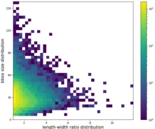
Target detection methods based on deep learning usually generate the predicted region proposals of the target at each position on the feature map. In order to reduce the number of predicted proposals, several fixed region proposals are given, which are called anchors. Anchor converts the object detection problem into the regression problem between each proposal and its assigned object box [45]. By this way, the problem of high detection miss rate caused by multiple objects in the same area can be solved. The size of anchor is critical to network performance. In the deeper layers of the feedforward network, the feature maps have more semantics, so that the anchor size is set larger to detect larger objects. The small anchor on the feature maps obtained by the shallow network is used to detect small objects. The SAR ship detection dataset used in this paper is of multi-resolution, and different types of ships have different sizes, so that the ship in the chips has various sizes. In addition, the SAR images are affected by the imaging mode, and the geometric deformation caused by the incidence angle will also result in the change of the ship shape in chips. Here, we use the multi-layer feature maps for ship detection, and we need to design the multiple anchor sizes for the SAR ship detection dataset. We count the distribution of the bounding box size in the dataset and take into account the comprehensive size and the aspect ratio of the bounding box. Taking plbbox×sbboxas the horizontal axis and lbbox
sbbox as the vertical axis, we locate each bounding box in a two-dimensional coordinate graph, so as to have a comprehensive understanding of the distribution of the bounding box size. Here,lbboxandsbboxare the lengths of the long side and the short side of each bounding box. The result is shown in Figure5.
Remote Sens. 2019, 11, x FOR PEER REVIEW 8 of 23
2.3. The Improvements on RetinaNet 2.3.2. Multi-Scale Anchor Design
Target detection methods based on deep learning usually generate the predicted region proposals of the target at each position on the feature map. In order to reduce the number of predicted proposals, several fixed region proposals are given, which are called anchors. Anchor converts the object detection problem into the regression problem between each proposal and its assigned object box [45]. By this way, the problem of high detection miss rate caused by multiple objects in the same area can be solved. The size of anchor is critical to network performance. In the deeper layers of the feedforward network, the feature maps have more semantics, so that the anchor size is set larger to detect larger objects. The small anchor on the feature maps obtained by the shallow network is used to detect small objects.
The SAR ship detection dataset used in this paper is of multi-resolution, and different types of ships have different sizes, so that the ship in the chips has various sizes. In addition, the SAR images are affected by the imaging mode, and the geometric deformation caused by the incidence angle will also result in the change of the ship shape in chips. Here, we use the multi-layer feature maps for ship detection, and we need to design the multiple anchor sizes for the SAR ship detection dataset. We count the distribution of the bounding box size in the dataset and take into account the comprehensive size and the aspect ratio of the bounding box. Taking lbboxsbbox as the horizontal
axis and b b o x b b o x
l
s as the vertical axis, we locate each bounding box in a two-dimensional coordinate graph, so as to have a comprehensive understanding of the distribution of the bounding box size. Here,
l
bbox ands
bbox are the lengths of the long side and the short side of each bounding box. The result is shown in Figure 5.Figure 5. The relative bounding-box size distribution of the training set.
In Figure 5, the color bar on the right represents the number of bounding boxes, and the number increases from blue to yellow. As shown in Figure 5, the sizes of most bounding boxes are regular with the comprehensive size of 30^2 and the aspect ratio between 1 and 2. Based on this, we re-design the size of the anchor. As mentioned in Section 2.1.1, in order to avoid high computational complexity, the feature maps {P2, P3, P4} are used for prediction. The anchors of deeper layers cover a huge area with respect to the network’s input image, which will only overlap a few huge objects. The size of the input SAR image is 256 × 256 and the anchors have the base areas of 16^2, 32^2, 64^2, respectively. At each pyramid level, the anchors have three aspect ratios {1:2, 1:1, 2:1}. For dense scale coverage, at each level we add anchors of sizes {0.4, 0.8, 1.2} of the original set of three aspect ratio anchors. In total, there are nine anchors per level and across levels they cover the scale range of 6.4–
Figure 5.The relative bounding-box size distribution of the training set.
In Figure5, the color bar on the right represents the number of bounding boxes, and the number increases from blue to yellow. As shown in Figure5, the sizes of most bounding boxes are regular with the comprehensive size of 30ˆ2 and the aspect ratio between 1 and 2. Based on this, we re-design the size of the anchor. As mentioned in Section2.1, in order to avoid high computational complexity, the feature maps {P2, P3, P4} are used for prediction. The anchors of deeper layers cover a huge area with respect to the network’s input image, which will only overlap a few huge objects. The size of the input SAR image is 256×256 and the anchors have the base areas of 16ˆ2, 32ˆ2, 64ˆ2, respectively. At each pyramid level, the anchors have three aspect ratios {1:2, 1:1, 2:1}. For dense scale coverage, at each level we add anchors of sizes {0.4, 0.8, 1.2} of the original set of three aspect ratio anchors. In total, there are nine anchors per level and across levels they cover the scale range of 6.4–76.8 pixels with
Remote Sens.2019,11, 2694 9 of 22
respect to the network’s input image. These anchors can cover most bounding boxes in the dataset, and will not result in a huge model with too many anchors.
2.3.2. Split Convolution Block (SCB)
In order to improve the feature extraction performance of small targets, we propose a new convolution block, namely, split convolution block (SCB); that is, the original input image is divided into several sub-images of the same size and used as the input of the network. In order to avoid the discontinuity of target features caused by some targets at the edge of clipping, here we still keep a normal convolution block and take the complete SAR image as input. At the same time, the overall characteristics of the input image are also what we need to pay attention to. After the first convolution module, the feature maps corresponding to the sub-images are spliced and fused with the feature maps of normal convolution. Through the combination of SCB and normal convolution, the feature extraction of target is obtained in a finer granularity so as to retain more detailed features and improve the detection accuracy of small targets.
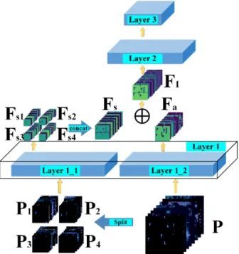
The inspiring idea of this paper is the global precedence in visual perception [46,47]. That is to say, most people are more sensitive to the overall features than the local details, which makes them neglect the key details when they pay attention to the target, especially the small targets. The operation object of convolution is the whole input image with convolution kernels of fixed sizes. When the region of interest is large, it is difficult for the network to obtain complete details of the target with limited convolution parameters, resulting in the loss of information. In order to reduce such an information loss caused by the global precedence and improve the network’s attention to SAR image details, SCB splits the large image into several small ones as the inputs of the network. The proportion of the target area in the small ones will be larger and the details will be more prominent. By processing the inputs of small size, the feature extraction of the target will be much easier. In this paper, we cut the input image into four sub-images of the same size, namely, the cutting positions are the middle of the distance and azimuth dimensions. The bottom-up pathway of FPN with SCB is shown in Figure6.
Remote Sens. 2019, 11, x FOR PEER REVIEW 9 of 23
76.8 pixels with respect to the network’s input image. These anchors can cover most bounding boxes in the dataset, and will not result in a huge model with too many anchors.
2.3.2. Split Convolution Block (SCB)
In order to improve the feature extraction performance of small targets, we propose a new convolution block, namely, split convolution block (SCB); that is, the original input image is divided into several sub-images of the same size and used as the input of the network. In order to avoid the discontinuity of target features caused by some targets at the edge of clipping, here we still keep a normal convolution block and take the complete SAR image as input. At the same time, the overall characteristics of the input image are also what we need to pay attention to. After the first convolution module, the feature maps corresponding to the sub-images are spliced and fused with the feature maps of normal convolution. Through the combination of SCB and normal convolution, the feature extraction of target is obtained in a finer granularity so as to retain more detailed features and improve the detection accuracy of small targets.
The inspiring idea of this paper is the global precedence in visual perception [46,47]. That is to say, most people are more sensitive to the overall features than the local details, which makes them neglect the key details when they pay attention to the target, especially the small targets. The operation object of convolution is the whole input image with convolution kernels of fixed sizes. When the region of interest is large, it is difficult for the network to obtain complete details of the target with limited convolution parameters, resulting in the loss of information. In order to reduce such an information loss caused by the global precedence and improve the network's attention to SAR image details, SCB splits the large image into several small ones as the inputs of the network. The proportion of the target area in the small ones will be larger and the details will be more prominent. By processing the inputs of small size, the feature extraction of the target will be much easier. In this paper, we cut the input image into four sub-images of the same size, namely, the cutting positions are the middle of the distance and azimuth dimensions. The bottom-up pathway of FPN with SCB is shown in Figure 6.
.
Figure 6. The bottom-up pathway of FPN embedded with SCB.
As shown in Figure 6, given the input SAR images C H W
P
, we cut them in half of W/H and
obtain four reduced sub-images 2 2( 1, 2, 3, 4)
H W C i
P i . Such a process can be summarized as:
Figure 6.The bottom-up pathway of FPN embedded with SCB.
As shown in Figure6, given the input SAR imagesP∈RC×H×W, we cut them in half of W/H and obtain four reduced sub-imagesPi∈RC×H2×W2 (i=1, 2, 3, 4). Such a process can be summarized as:
Remote Sens.2019,11, 2694 10 of 22
Pi=split(split(P)H
2)W2 (i=1, 2, 3, 4) (9)
After that, we inputPandPi(i=1, 2, 3, 4)into the first convolution module of the network and obtain feature mapsFa∈Rc×h×wandFsi∈Rc×h2×w2(i=1, 2, 3, 4), respectively. The relative position of
Fsi(i= 1, 2, 3, 4)is shown in Figure6. After obtaining the four groups of feature maps of SCB, we first concatenate them at the corresponding channel and spatial position to obtain the feature maps Fs∈Rc×h×wwith the same size as the feature mapsFa∈Rc×h×wof normal convolution. The splicing process can be expressed as Equation (10).
Fs=concat(concat(Fs1,Fs2)w
2),concat(Fs3,Fs4)w2))h2 (10)
whereconcat(•)w
2,concat(
•)h
2 denotes concatenating at the position of
w
2,h2. After that,FaandFsare added on the corresponding channel, generating the optimized feature mapsF1∈Rc×h×w.
F1=Fa⊕Fs (11)
where⊕denotes adding element-by-element at the corresponding convolution channels.
The optimized feature mapsF1∈Rc×h×ware used as the input of the next convolution module. In this way, SAR image feature extraction is enhanced.
2.3.3. Spatial Attention Block (SAB)
We embed SAB in FPN to optimize the performance of the network from the perspective of the attention mechanism. SAB efficiently helps the information flow within the network by learning which information to emphasize or suppress. The location of SAB in FPN is shown in Figure1. As shown in Figure4, in FPN, when the feedforward network (bottom-up pathway) and the feature pyramid net (top-down pathway) are connected, 1×1 convolution is adopted to reduce the feature map channels to a fixed number 256. Through such a design, the feedforward network and the other parts of FPN are separated so that the change of the feedforward network structure will not affect the feature pyramid net, box and class subnets. In addition, the network will be more compact with the help of dimensionality reduction with 1×1 convolution. FPN realizes the target detection based on the feature maps of multiple layers and too many feature maps will make the network architecture too large and take a long time to train.
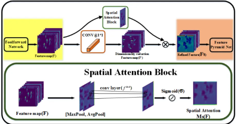
Basically, 1×1 convolution has two main functions. One is to realize the cross-channel interaction and information integration of feature maps in different channels, so as to improve the expression ability of the network. The second is to reduce or increase the number of feature map channels, so as to increase the nonlinearity of CNNs and facilitate the optimization of network structure. The 1×1 convolution simply maps the values at the same location of all channels to one value, without considering the spatial information along the W/H dimension of the feature maps. For the purpose of enlarging the receptive field of 1×1 convolution, Inception adds 3×3 and 5×5 convolution in parallel to obtain the receptive field of different sizes and extract the features on different scale. However, the increase of the network width results in the degradation of the network computational performance. In order not to significantly increase the computational complexity, we embed SAB in FPN to enhance the spatial information on the feature maps [48,49]. SAB infers a 2D spatial attention map and refines the feature maps of the feedforward network. By multiplying the spatial attention map and the feature maps with channel reduced by 1×1 convolution, the feature maps refined on spatial-wise will obtained. The location and specific implementation process of SAB are shown in Figure7.
Remote Sens.2019,11, 2694 11 of 22
Remote Sens. 2019, 11, x FOR PEER REVIEW 11 of 23
Figure 7. The location of SAB in FPN and the diagram of SAB.
Here, we take the feature maps output by the feedforward network 1
c h w
F
as an example to introduce the whole implementation process in detail. Firstly, the dimensionality reduced featuremap 1
c h w
F
is obtained by the convolution with 1 × 1 kernel. 1 11
( )
1F
f
F
(15)where
f
1 1denotes the convolution with the kernel of size 1 1 .
In addition to 1 × 1 convolution, we also input
F
1 into SAB. The specific approach is to makeglobal average pooling and global max-pooling along the channel axis of
F
1 so as to obtain thepooling result with a size of hw, and a channel of 2. After that, we concentrate on the pooling result
and generate an efficient feature descriptor. As shown in Figure 7, on the concatenated feature descriptor, a
a a
kernel is applied to generating a spatial attention map
11
M Fs h w
which
encodes where to emphasize or suppress. The process of getting M Fs
1 can be summarized asfollows:
1
1 1
1 1M F
s
(
f
a a( Avgpool(F );Maxpool(F ) ))
(
f
a a( F ;F
avgs maxs
))
(16)where
denotes the sigmoid function andf
a a denotes the convolution with a kernel of sizea a
. We take the kernel size of 3 × 3 in SAB of our model.By multiplying the spatial attention map M Fs
1 and dimensionality reduced feature mapsF
1
, the output feature maps refined on spatial-wise 1c h w s
F
can be obtained:
1 1 1 Fs Ms F F (17)where denotes element-wise multiplication.
By this way, we transfer the feature maps with enhanced spatial features to the feature pyramid net for feature fusion. One can seamlessly integrate SAB in FPN with a slight modification and SAB will not change the convergence of baseline model. With the lightweight architecture of SAB, the increased running time of SAB can be neglected which is verified in the experiments section.
Figure 7.The location of SAB in FPN and the diagram of SAB.
Here, we take the feature maps output by the feedforward networkF1∈Rc×h×was an example to introduce the whole implementation process in detail. Firstly, the dimensionality reduced feature map F10∈Rc
0×
h×w
is obtained by the convolution with 1×1 kernel. F1
0
= f1×1(F1) (12)
where f1×1denotes the convolution with the kernel of size 1×1.
In addition to 1×1 convolution, we also inputF1into SAB. The specific approach is to make global average pooling and global max-pooling along the channel axis ofF1so as to obtain the pooling result with a size ofh×w, and a channel of 2. After that, we concentrate on the pooling result and generate an efficient feature descriptor. As shown in Figure7, on the concatenated feature descriptor, a a×akernel is applied to generating a spatial attention mapMs(F1)∈R1×h×w
which encodes where to emphasize or suppress. The process of gettingMs(F1)can be summarized as follows:
Ms(F1) =σ(fa ×a ([Avgpool(F1); Maxpool(F1)])) =σ(fa ×a (hF1savg;F1smax i )) (13)
whereσdenotes the sigmoid function and fa×adenotes the convolution with a kernel of sizea×a. We take the kernel size of 3×3 in SAB of our model.
By multiplying the spatial attention mapMs(F1)and dimensionality reduced feature mapsF10, the output feature maps refined on spatial-wiseF1s∈Rc
0× h×w can be obtained: F1s=Ms(F1)⊗F1 0 (14) where⊗denotes element-wise multiplication.
By this way, we transfer the feature maps with enhanced spatial features to the feature pyramid net for feature fusion. One can seamlessly integrate SAB in FPN with a slight modification and SAB will not change the convergence of baseline model. With the lightweight architecture of SAB, the increased running time of SAB can be neglected which is verified in the experiments section.
3. Results and Discussions 3.1. Configuration
3.1.1. Dataset Description
The dataset used in this paper is a SAR dataset for ship detection published by the Digital Earth Laboratory of the Aerospace Information Research Institute, Chinese Academy of Sciences [50]. There are 102 GaoFen-3 images and 108 Sentinel-1 images that are used to constructed the dataset. As for
Remote Sens.2019,11, 2694 12 of 22
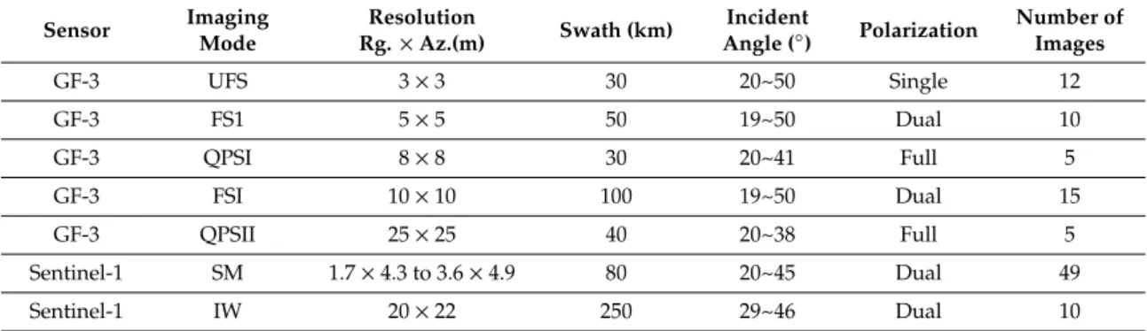
GaoFen-3, the resolution of these images involves 3 m, 5 m, 8 m and 10 m with Strip-Map (UFS), Fine Strip-Map 1 (FSI), Full Polarization 1 (QPSI), Full Polarization 2(QPSII) and Fine Strip-Map 2 (FSII) imaging mode, respectively. The Sentinel-1 imaging modes are S3 Strip-Map (SM), S6 SM and IW-mode. The details of these images are shown in Table1, including imaging mode, resolution, incidence angle and polarization.
Table 1.The quantitive detection results Detailed information for original SAR imagery.
Sensor Imaging Mode Resolution Rg.×Az.(m) Swath (km) Incident Angle (◦) Polarization Number of Images GF-3 UFS 3×3 30 20~50 Single 12 GF-3 FS1 5×5 50 19~50 Dual 10 GF-3 QPSI 8×8 30 20~41 Full 5 GF-3 FSI 10×10 100 19~50 Dual 15 GF-3 QPSII 25×25 40 20~38 Full 5 Sentinel-1 SM 1.7×4.3 to 3.6×4.9 80 20~45 Dual 49 Sentinel-1 IW 20×22 250 29~46 Dual 10
Based on these preprocessed SAR images, sliding windows are used to acquire ship chips of 256×256 pixels in size. In order to enrich the backgrounds of these chips, adjacent sliding windows have overlapping of 128 pixels in both horizontal and vertical directions. Currently, there are 43,819 ship chips in this dataset and each ship chip is labeled by SAR experts.
From Figure8, we can see that the dataset has the following three characteristics. First, there are multi-size SAR ships in these chips, and the size conversion range is large. Second, there are complex backgrounds in the ship chips. Some of ships are on the open sea, some in the port. Third, the distribution of these ships has many forms, including independent cruising and fleet sailing. All of these have brought difficulties to ship detection, and put forward higher requirements for the performance of ship detection. In the experiment, we divide the training and testing set randomly according to the rate of 7:3. A total of 30,673 ship chips are used for training and 13,146 ship chips are used for testing.
Remote Sens. 2019, 11, x FOR PEER REVIEW 13 of 23
Figure 8. Some samples of ship chips. (a), (b), (c), (d) and (e) are cropped from Gaofen-3 images. (f),
(g), (h), (i) and (j) are cropped from Sentinel-1 images.
3.1.2. Evaluation Metrics
In order to make a quantitative evaluation of the experimental results, we adopt four widely used criteria, namely, precision, recall, mAP (mean Average Precision) and F1 score. The precision measures the fraction of detections that are true positives and the recall measures the fraction of positives over the number of ground-truths, given by [51].
TP TP FP TP TP FN N precision N +N N recall N +N (18)
where
N
TP,N
FP andN
FN represent the number of true positives, the number of false positives and the number of false negatives.As for object detection, a higher precision and a higher recall are both expected. Whereas, in fact, precision and recall are a pair of contradictory indicators. It means that a higher precision will result in a lower recall and a higher recall will result in a lower precision. F1 score is a commonly used criteria in object detection, which can comprehensively evaluate precision and recall. A higher F1 score means a more ideal comprehensive detection performance [52]. F1 score is defined based on the harmonic average of precision and recall:
2 precision recall
F1
precision+recall
(19)
Precision, recall and F1 score are all calculated based on the single point threshold. mAP can solve the limitations of single point threshold and get an indicator that reflects the global performance. mAP is obtained by the integral of the precision over the interval from recall=0 to recall=1, that is, the area under the precision-recall (PR) curve [53].
1 0
mAP=
P(R)dR (20)3.2. Experiment Results
The baseline model used in this paper is RetinaNet. In order to verify the effectiveness of the proposed SCB and SAB, we conduct the following comparison experiments under four conditions: RetinaNet, SAB-RetinaNet (RetinaNet embedded with SAB), SCB-RetinaNet (RetinaNet embedded with SCB), 2S-RetinaNet (RetinaNet embedded with SAB and SCB). The bottom-up pathway of FPN
(j) (i) (h) (g) (e) (d) (c) (b) (a) (f) (b)
Figure 8.Some samples of ship chips. (a), (b), (c), (d) and (e) are cropped from Gaofen-3 images. (f), (g), (h), (i) and (j) are cropped from Sentinel-1 images.
3.1.2. Evaluation Metrics
In order to make a quantitative evaluation of the experimental results, we adopt four widely used criteria, namely, precision, recall, mAP (mean Average Precision) and F1 score. The precision measures
Remote Sens.2019,11, 2694 13 of 22
the fraction of detections that are true positives and the recall measures the fraction of positives over the number of ground-truths, given by [51].
precison= NTP NTP+NFP recall= NTP NTP+NFN (15)
whereNTP,NFPandNNFrepresent the number of true positives, the number of false positives and the number of false negatives.
As for object detection, a higher precision and a higher recall are both expected. Whereas, in fact, precision and recall are a pair of contradictory indicators. It means that a higher precision will result in a lower recall and a higher recall will result in a lower precision. F1 score is a commonly used criteria in object detection, which can comprehensively evaluate precision and recall. A higher F1 score means a more ideal comprehensive detection performance [52]. F1 score is defined based on the harmonic average of precision and recall:
F1=2× precison×recall
precison+recall (16)
Precision, recall and F1 score are all calculated based on the single point threshold. mAP can solve the limitations of single point threshold and get an indicator that reflects the global performance. mAP is obtained by the integral of the precision over the interval from recall=0 to recall=1, that is, the area under the precision-recall (PR) curve [53].
mAP=
Z 1
0
P(R)dR (17)
3.2. Experiment Results
The baseline model used in this paper is RetinaNet. In order to verify the effectiveness of the proposed SCB and SAB, we conduct the following comparison experiments under four conditions: RetinaNet, SAB-RetinaNet (RetinaNet embedded with SAB), SCB-RetinaNet (RetinaNet embedded with SCB), 2S-RetinaNet (RetinaNet embedded with SAB and SCB). The bottom-up pathway of FPN under each condition consists of the same ResNet. At the beginning of network training, we use the parameters pre-trained on ImageNet to initialize the network and fine-tune the system on this bias [54]. We train 100 iterations under each experiment condition, and all the other training parameters are consistent. During the training and testing process, the IoU (Intersection over Union) value adopts a uniform 0.5, that is, the ratio of the intersection and the union between the candidate bounding box and the ground truth should be greater than or equal to 0.5. The IoU value will affect the precision and recall of object detection, especially the recall. A high IoU value will lead to a low recall and 0.5 is the common used value for object detection. The PR curves of the four experiments are plotted in Figure9. The x and y axes are the recall and precision.
Remote Sens.2019,11, 2694 14 of 22
Remote Sens. 2019, 11, x FOR PEER REVIEW 14 of 23
under each condition consists of the same ResNet. At the beginning of network training, we use the parameters pre-trained on ImageNet to initialize the network and fine-tune the system on this bias [54]. We train 100 iterations under each experiment condition, and all the other training parameters are consistent. During the training and testing process, the IoU (Intersection over Union) value adopts a uniform 0.5, that is, the ratio of the intersection and the union between the candidate bounding box and the ground truth should be greater than or equal to 0.5. The IoU value will affect the precision and recall of object detection, especially the recall. A high IoU value will lead to a low recall and 0.5 is the common used value for object detection. The PR curves of the four experiments are plotted in Figure 9. The x and y axes are the recall and precision.
Figure 9. The PR curves of the four methods.
On the PR curves, if one algorithm is completely encased by another algorithm, it means that the performance of the latter is better than the former. As shown in Figure 9, in most areas of the PR curves, RetinaNet is located inside the other three algorithms. When both SAB and SCB are embedded into RetinaNet, the network performance is greatly improved, and its PR curve is located at the outermost side, enclosing all three algorithms. The training and testing sets are divided randomly, and the data feature distribution domains are basically consistent. So, In Table 2, we show the detailed detection results on the testing set of the four methods. The main configurations of the employed computer are GPU: GTX 1060; 2.8 GHz; 8GB RAM; operating system: Ubuntu 16.04; running software: Python 2.7. The computational efficiency of the methods is reflected by the average testing time per image in the last column of Table 2.
Table 2. The quantitative detection results on the testing set.
Methods Precision Recall F1 Score mAP
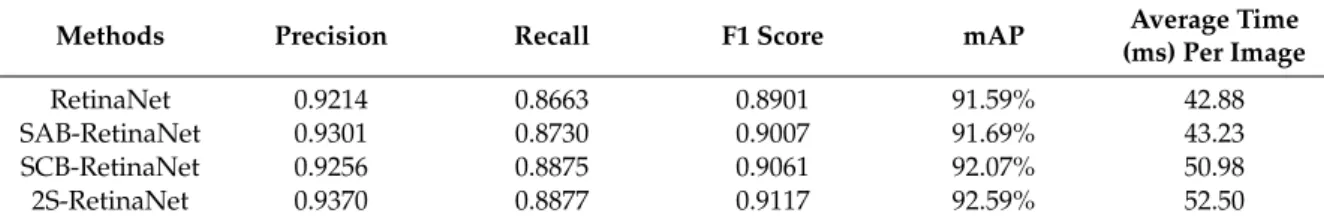
Average Time(ms) Per Image RetinaNet 0.9214 0.8663 0.8901 91.59% 42.88 SAB -RetinaNet 0.9301 0.8730 0.9007 91.69% 43.23 SCB -RetinaNet 0.9256 0.8875 0.9061 92.07% 50.98 2S-RetinaNet 0.9370 0.8877 0.9117 92.59% 52.50
In Table 2, precision and recall are affected by the specific threshold, here, precision and recall are obtained at the highest F1 score. Through the four indicators, we can see that the performance of RetinaNet has been improved, whether SAB or SCB is embedded. The performance of 2S-RetinaNet is better than the other three algorithms, which can explain that in Figure 9, RetinaNet is basically located in the innermost part of the four PR curves, and 2S-RetinaNet is located outermost. From the average time per image, we can see that the after SAB and SCB are embedded, the computation load
Figure 9.The PR curves of the four methods.
On the PR curves, if one algorithm is completely encased by another algorithm, it means that the performance of the latter is better than the former. As shown in Figure9, in most areas of the PR curves, RetinaNet is located inside the other three algorithms. When both SAB and SCB are embedded into RetinaNet, the network performance is greatly improved, and its PR curve is located at the outermost side, enclosing all three algorithms. The training and testing sets are divided randomly, and the data feature distribution domains are basically consistent. So, In Table2, we show the detailed detection results on the testing set of the four methods. The main configurations of the employed computer are GPU: GTX 1060; 2.8 GHz; 8GB RAM; operating system: Ubuntu 16.04; running software: Python 2.7. The computational efficiency of the methods is reflected by the average testing time per image in the last column of Table2.
Table 2.The quantitative detection results on the testing set.
Methods Precision Recall F1 Score mAP Average Time
(ms) Per Image
RetinaNet 0.9214 0.8663 0.8901 91.59% 42.88
SAB-RetinaNet 0.9301 0.8730 0.9007 91.69% 43.23
SCB-RetinaNet 0.9256 0.8875 0.9061 92.07% 50.98
2S-RetinaNet 0.9370 0.8877 0.9117 92.59% 52.50
In Table2, precision and recall are affected by the specific threshold, here, precision and recall are obtained at the highest F1 score. Through the four indicators, we can see that the performance of RetinaNet has been improved, whether SAB or SCB is embedded. The performance of 2S-RetinaNet is better than the other three algorithms, which can explain that in Figure9, RetinaNet is basically located in the innermost part of the four PR curves, and 2S-RetinaNet is located outermost. From the average time per image, we can see that the after SAB and SCB are embedded, the computation load of the network increases, which is reflected in the increase of testing time. The computation efficiency of these algorithms are of the same order of magnitude. The increased computation is mainly concentrated in SCB, while the increased computation in SAB is small. In the following Section3.3, we will make a specific visual analysis on the two modules of SAB and SCB.
3.3. Discussion
In this section, the functions and principles of SCB and SAB are visualized to verify their effectiveness. Here, 2S-RetinaNet is used for experiments. The number of iterations of training, dataset and model configurations used are consistent with those described in Section3.1.