04 August 2020
Repository ISTITUZIONALE
Learning and Adapting Robust Features for Satellite Image Segmentation on Heterogeneous Datasets / Ghassemi, Sina; Fiandrotti, Attilio; Francini, Gianluca; Magli, Enrico. - In: IEEE TRANSACTIONS ON GEOSCIENCE AND REMOTE SENSING. - ISSN 1558-0644. - STAMPA. - 57:9(2019), pp. 6517-6529.
Original
Learning and Adapting Robust Features for Satellite Image Segmentation on Heterogeneous Datasets
ieee Publisher: Published DOI:10.1109/TGRS.2019.2906689 Terms of use: openAccess Publisher copyright
copyright 20xx IEEE. Personal use of this material is permitted. Permission from IEEE must be obtained for all other uses, in any current or future media, including reprinting/republishing this material for advertising or promotional purposes, creating .
(Article begins on next page)
This article is made available under terms and conditions as specified in the corresponding bibliographic description in the repository
Availability:
This version is available at: 11583/2730891 since: 2019-09-27T12:22:44Z
Learning and Adapting Robust Features for
Satellite Image Segmentation on
Heterogeneous Datasets
Sina Ghassemi,
Sudent Member, IEEE,
Attilio Fiandrotti,
Member, IEEE,
Gianluca Francini,
and Enrico Magli,
Fellow, IEEE
Abstract—This work addresses the problem of training a deep neural network for satellite image segmentation so that it can be deployed over images whose statistics differ from those used for training. For example, in post-disaster damage assessment, the tight time constraints make it impractical to train a network from scratch for each image to be segmented. We propose a convolutional encoder-decoder network able to learn visual representations of increasing semantic level as its depth increases, allowing it to generalize over a wider range of satellite images. Then, we propose two additional methods to improve the network performance over each specific image to be segmented. First, we observe that updating the batch normalization layers statistics over the target image improves the network performance without human intervention. Second, we show that refining a trained network over a few samples of the image boosts the network performance with minimal human intervention. We evaluate our architecture over three datasets of satellite images, showing state-of-the-art performance in binary segmentation of previously unseen images and competitive performance with respect to more complex techniques in a multiclass segmentation task.
Index Terms—Deep learning, convolutional neural network, encoder-decoder architecture, satellite image segmentation, do-main adaptation.
I. INTRODUCTION
S
ATELLITE image segmentation has received lots of at-tention lately due to the availability of annotated high resolution image datasets captured by the last generation of satellites. The problem of segmenting a satellite image can be defined as classifying (or labeling) each pixel of the image according to a number of classes such as buildings, roads, water and so on (semantic pixel labeling). Recent research in semantic pixel labeling builds upon and leverages recent advances [1] in supervised image classification achieved with Convolutional Neural Networks (CNNs) [2]. CNNs are artificial feed-forward, acyclic, neural networks typically com-posed of a feature extraction stage followed by a classification stage. The feature extraction stage consists of multiple stacked convolutional layers, where each layer includes multiple learn-able filters. When CNNs are trained end-to-end via error gradient backpropagation, the convolutional layers learn to detect features of increasingly higher semantic level that are eventually classified by one or more fully connected layers.This work tackles the challenging case where the segmen-tation algorithm is to be deployed over images that are not known at training time. Indeed, most CNN-based schemes for satellite image segmentation focus on the case where the
network is trained (from scratch) over images similar to those where the algorithm is to be deployed [3], [4], [5], [6], [7], [8]. However, if training and test images are captured by different sensors or at different time intervals or locations, they exhibit different statistics, an issue known as covariate shift [9]. In some applications such as emergency mapping, satellite images must be segmented in a short time in the aftermath of events such as flood, or earthquake. In similar scenarios, the tight time constraints prompt for solutions that allow reusing some algorithm previously trained over different images.
A number of approaches have been devised to address the domain adaptation problem, where an algorithm trained over samples with some input distribution (source domain) is to operate over samples with different distribution (target domain) [10]. Some approaches rely on selecting a subset of features which are invariant to the shift in domain [11], [12]. Other approaches focus on data distributions of target and source domain and they aim to make these domains statistically similar to keep the classifier unchanged [13], [14], [15], [16]. Other methods rely on adaptation of classifier rather than data distributions across domains [17], [18]. In addition, inspired by the generative adversarial networks (GAN) [19], some recent studies have been carried out in order to learn representations which are invariant to domain shift with the aid of an additional adversarial term to the total cost function.[20], [21]. Whereas domain adaptation techniques have been proven successful in image classification, they have received little attention for satellite image segmentation, leaving the covariate shift issue largely open.
In this study, we propose a CNN-based architecture to address segmentation over heterogeneous datasets which are affected by covariate shift. In order to minimize the adverse effect of covariate shift on the segmentation performance, first we optimize the network architecture for better generalization ability, then we propose two domain adaptation techniques to enhance the performance over each image under study. Regarding the proposed network, we design an architecture composed of anencodernetwork and adecodernetwork. The encoder is based on a residual architecture [22] that enables convolutional topologies deep up to hundreds of layers [23], [24]. As the encoder gets deeper and learns to detect more features, it can be trained over larger numbers of dissimilar images to detect features of higher semantic level. As a result, the learned features are less specific to the training images and are more likely to be useful to segment images
unseen at training time, improving the encoder generalization ability. Intermediate layers of the encoder and the decoder are linked with skip connections [25] which allow dealing with features of different semantic level. The network is trained over images potentially very different from those to be segmented at deployment time. Regarding the domain adaptation, we devise two solutions for adapting the trained network over each specific image to be segmented when deployed on the field. First, we show that updating the batch normalization (BN) layers statistics on the deployment images is effective towards normalizing the inputs to convolutional layers. Second, refining the network parameters over small regions of the images where it is to be deployed improves segmentation accuracy with little additional manual effort. The performance of the proposed architecture is experimentally evaluated over two publicly available and one homegrown dataset of annotated satellite images. Our experiments show that as the encoder depth increases (up to 151 layers), the segmentation accuracy improves. Moreover, a residual encoder performs and generalizes better with respect to a deeper plain convolutional encoder. Adaptation experiments also show that updating the batch normalization statistics offers gains up to 0.5% and close to 3% in terms of overall segmentation accuracy and F1-Score. Refining the trained network boosts the above gains to 1% and 6% respectively when about one-third of the image to be segmented is hand-annotated. This work builds upon and extends our preliminary research [26] in multiple directions. First, we propose a simple yet effective strategy for adapting a trained network that consists upon re-fining the batch normalization (BN) statistics over each image to segment. Second, we extend the experimental validation of our architecture over two publicly available datasets of satellite images, comparing our method to state-of-the-art techniques.
The rest of this article is organized as follows. Section II discusses the recent literature in the field and the major shortcomings of existing approaches. Sec. III briefly overviews the background relevant to this work. Sec. IV describes our proposed architecture, whereas Sec. V describes the related training procedure. Sec. VI presents two domain adaptation methods to improve the performance of a trained network over specific images. Finally, in Sec. VII we experimentally assess the performance of our proposed architecture over three distinct datasets of satellite images. Conclusions are drawn in Sec. VIII.
II. RELATEDWORK
Automatic segmentation of hyperspectral satellite images has been the subject of extensive studies over the past decade. Mainstream approaches rely on manually designing class-specific features extractors where the extracted features are further classified for image segmentation. Morphological index and Pixel Shape Index (PSI) [27], [28], [29] are among the best known families of hand-crafted features proposed in the litera-ture. Concerning feature classification, discriminative learning [30], [31], [32] aims at discovering the informative subspace within feature domain to improve the classifier performance. Concerning feature classification, mainly the support vector
machine [33] is deployed to process the generated features and perform final decision over pixels of the image.
Fostered by the availability of large annotated images and leveraging the computational capabilities of modern GPUs, a number of approaches based on deep convolutional architec-tures have been proposed recently for image segmentation.
Farabet et al.[34] proposed a multi-scale CNN to address scene labeling. Their proposed architecture consists of three convolutional branches each working on a specific scale of input image generated by a Laplacian pyramid. The output feature maps of these branches are scaled up to recover the original size of the input and then concatenated over the three scales. Finally the segmentation results of convolutional branches are used by super-pixel algorithm or conditional random field in order to predict the final segmentation and to enforce spatial consistency.
Longet al.[35] introduced a fully CNN for image segmen-tation which takes an input of arbitrary size. Coarse feature maps from deeper layers are combined with those in early layers and with finer resolution which contributes to more precise segmentation.
In the medical imaging domain, Ronneberger et al. [25] devised an architecture called U-Netcomposed of a contract-ing branch consistcontract-ing of convolutional layers and a symmetric expanding branch including deconvolution layers. The con-tracting path processes the input image through convolution and pooling layers producing coarse feature maps. In the expanding part, these feature maps are scaled up using decon-volution operations to match the input size and produce the score maps over segmentation classes. Skip connections are used to help the flow of information between these two parts contributing to precise fine segmentation. Ghiasi et al. [36] deployed a similar multi-resolution reconstruction architecture built upon a Laplacian pyramid. The coarse feature maps are refined through the reconstruction branch by fusing feature maps with the information of early layers in the network.
Chen et al. [37] introduced Deeplab, a CNN in which atrous convolution is employed to address image segmentation. Atrous convolution helps to enlarge the field of view of feature maps while keeping their resolution the same. Moreover, atrous spatial pyramid pooling is employed to add multi-scale content to feature maps. In the end, authors implemented fully connected conditional random fields to refine CNN outputs and perform the segmentation.
Pushed by the success scored with natural images segmen-tation, a number of methods for satellite image segmentation have been proposed recently.
Authors in [3] addressed semantic labelling over Vaihingen city using patch-based CNN and also fully convolutional architecture. To overcome the imbalanced classes, authors introduce a cross-entropy loss function weighted by median frequency balancing which results in better performance in less frequent classes like cars.
In [4] a downsample-then-upsample architecture similar to [25] is devised utilizing deconvolutional layers in order to tackle semantic labelling of Vaihingen and Potsdam cities. Good performance is achieved over the validation set.
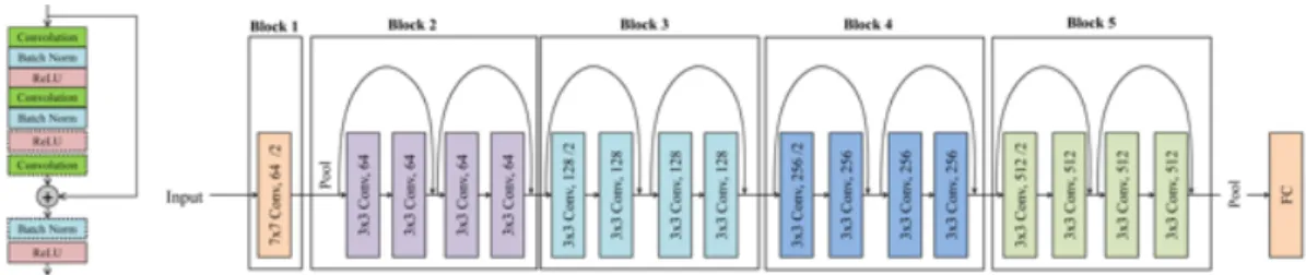
Fig. 1: Left: Architecture of a residual unit (dashed layers are found only in ResNets with 50 layers). Right: ResNet-18 topology with subdivision in residual blocks and further in residual units.
A multimodal architecture operating on infrared, red, green and digital surface model with multi-scale encoders is pro-posed in [5] which advances the state-of-the-art over Vaihingen dataset by fusing segmentation results obtained on three scales. [6] presents an edge-detection network to combine the pre-diction of class boundaries with the segmentation score maps to increase the segmentation precision. They evaluated their approach over Vaihingen and Potsdam datasets and improved the baseline performance. In [8] hand-crafted features are fused with features predicted by a CNN architecture, and a conditional random field inference is employed to make final predictions.
Authors in [38] propose a transfer learning approach to address the satellite image classification by refining a pre-trained CNN over novel dataset. They show that training the fully connected layers first, then refining the whole network using different learning rates for different network layers results in better performance.
Although most of the studies yield sufficiently accurate segment maps, few of them address the problem of deploying the trained network over images with different statistics from those used for training. In this work, we tackle such issue designing a network that can be trained to generalize over unseen images and methods to further improve its performance with respect to each image to be segmented.
III. RESIDUALNETWORKS
Residual networks (ResNets in the following) [22] are a class of deep convolutional networks that won the 2015 ImageNet large scale visual recognition contest. ResNets ad-dress the exploding/vanishing gradients problem [23], [24] in deep neural networks [39] by introducing skip connections which ease the backpropagation of the error gradients. The elementary unit of a ResNet is illustrated in Figure 1 and consists of two (or three) convolutional layers with 3⇥3 or 1⇥1 filters and Rectified Linear Unit (ReLU) [40] activation functions. During the forward pass, the skip connection sums the input of the unit to the output. At training time, the skip connection allows the error gradients to back-propagate from the output layer to layers closer to the network input. As a results, ResNets enable training much deeper architectures before running into vanishing gradients problems compared to standard convolutional networks. Multiple residual units are stacked together to form a residualblock, and a standard ResNet includes five blocks. ResNets lack pooling layers for
feature map spatial subsampling: the filters in the first convo-lutional layer of each block have a stride of two, effectively halving the feature maps resolution. Although the size of the feature maps is constant within each block, the number of feature maps output by a block depends on the overall ResNet depth as shown in Table I. Finally, a 7⇥7 average pooling layer reduces the dimensionality of the feature maps output by the last residual block, whereas one single fully connected layer takes care of the final image classification.
Finally, the figure shows that the inputs to the ReLU activations are normalized via batch normalization [41], a strategy addressing the internal covariate shift in multilayer neural networks. Let us consider the common case where saturating activations such as sigmoids or hyperbolic tangents are employed. If the inputs to the activation functions are not normalized, the activations are more likely to operate in the nonlinear region, thereby slowing down the training, whereas exploding gradients will require conservative learning rates, further slowing down the training. While we postpone to Sec. VI the details of batch normalization, in a nutshell it speeds up the training by normalizing the inputs to each activation function. This normalization is performed accord-ing to the input statistics learned duraccord-ing trainaccord-ing and yields higher learning rates. ResNets in particular rely on batch normalization because of their very deep architectures that demand sustained learning rates to be trained in reasonable time. In Sec. 3 we will show however that in a covariate shift scenario as in our case, batch normalization may hinder the network performance, which is the reason why we propose the adaptation strategy in Sec. VI-A.
TABLE I: Number of (output feature maps, convolutional layers) for each encoder (top) and decoder (bottom) block.
Encoder Num. of (feature maps, conv. layers) in encoder block depth Block 1 Block 2 Block 3 Block 4 Block 5
18 (64, 1) (64, 4) (128, 4) (256, 4) (512, 4) 34 ” (64, 6) (128, 8) (256, 12) (512, 6) 50 ” (256, 9) (512, 12) (1024, 18) (2048, 9)
101 ” ” ” (1024, 69) ”
152 ” ” (512, 24) (1024, 108) ” Encoder Num. of (feature maps, conv. layers) in decoder block
depth Block 1 Block 2 Block 3 Block 4 Block 5 18,34 (256, 1) (128, 1) (64, 1) (64, 1) (64, 1)
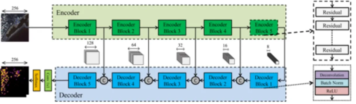
Fig. 2: Proposed encoder-decoder convolutional architecture for satellite image segmentation. The architecture of the encoder blocks and units is detailed in the dashed boxes. The architecture of the decoder blocks is detailed in the dotted boxes. ’C’ stands for the concatenation of feature maps.
IV. PROPOSEDARCHITECTURE
Our proposed architecture is shown in Fig. 2 and is com-posed of one encoder network paired with a decoder network. The encoder takes as input the image to be segmented and generates feature maps of different semantic level with differ-ent resolution. The decoder takes as input such feature maps and outputs a segmentation map, where each pixel is labeled according to one of the possible land usage classes. The rest of this section details the architecture and the operations of the encoder and the decoder, whereas the related training procedures are detailed in the next section.
A. Encoder
The upper part of Fig. 2 illustrates the architecture of the encoder, which is composed of five residual blocks, as detailed in the dashed box. We recall that the first convolutional layer of each block of a ResNet has a stride of two pixels. Therefore, each block outputs feature maps whose resolution is halved with respect to the feature maps taken as input. On the other hand, the number of output feature maps increases at each block. For example, the first block of the encoder takes as input a 256 ⇥256 ⇥D image, where D is the
number of spectral or color channels, and outputs64 feature
maps of resolution 128⇥128. Table I details the number
of feature maps output by each block and the number of convolutional layers in the block. As a result, the field of view of the convolutional filters increases at each block, allowing them to learn visual representations across different spatial ranges. Whereas the encoder design pattern follows that of a ResNet, a number of differences can be noticed with respect to Fig. 1. First, the pooling layer found in standard ResNets after the 5-th block is omitted to avoid an unneeded loss of spatial information. Second, we obtain a fully convolutional architecture by dropping the fully connected layer found in standard ResNets. In principle, this allows the network to efficiently process input images of arbitrary size without the need for shifting and stitching. Third and most important, the output of each block is not just provided as input to the following block, but is also provided as input to a specific block of the decoder unit. Providing feature maps extracted at multiple scales helps the decoder to refine its output as detailed in the following.
Our choice to design the encoder around a residual architec-ture rather than a plain convolutional one is meant to improve the network ability to generalize over wider range of images. Our conjecture is that the deep residual encoder is able to learn a large number of filters at different semantic levels, which we hypothesize is helpful towards coping with images whose statistics differ from training images. In Sec. VII the connection between residual encoder depth and the network generalization ability will be verified experimentally.
B. Decoder
The lower part of Fig. 2 illustrates the architecture of the decoder, which is composed of five deconvolutional blocks symmetric to the five residual blocks of the encoder. Each decoder block includes one deconvolutional layer, one batch normalization [41] layer and ReLU activations, as illustrated in the dotted box in Fig. 2. Deconvolutional layers (backward convolution) were originally proposed to address the loss of mid-level cues [42] caused by pooling operators used in convolutional networks. Each deconvolutional layer contains one or more deconvolutional filters, where each filter can be interpreted as a learnable upsampling function. Deconvolution works in two steps: first a sparse feature map is generated by interleaving zeros within the pixels, thereby upsampling the input feature maps by a specific factor (unpooling). Next, a dense feature map is generated by applying a convolution filter to the sparse feature map. Thus, each decoder block reverses the subsampling operation performed by the first convolutional layer of each encoder block.
Skip connections contribute to more precise and finer pre-dictions as the spatial information of early layers in encoder is used as well. Thus, feature maps output by each decoder block are concatenated with the feature maps produced by the corresponding encoder block. Notice that the number of feature maps coming from previous block and those from skip connections remains identical. We experimentally verified that this prevents one group of feature maps from dominating the other when they are concatenated and provided as input to the next deconvolutional block.
For the sake of clarity, we exemplify the operations of the
1-st decoder block with reference to a 18-layers encoder. The 1-st decoder block takes as input the 5128⇥8 feature maps
generated by the5-th encoder block. The feature maps are then scaled up by a factor of two by the 256 deconvolutional layers, reaching a 16⇥16 resolution. Such 256 feature maps are then concatenated with the identically sized 256 feature maps generated by the 4-th encoder block. The 512 concatenated
16⇥16feature maps are provided as input to the2-nd decoder block, and so forth. The decoder output finally consists of 64 feature maps with the size of256⇥256.
Next, the decoder output is processed by a convolutional layer with C filters (where C is the number of land classes)
of size 1 ⇥1. The output of such layer consists inC feature
maps of size256⇥256pixel: thei-th pixel in thek-th feature
mapoi,k(k2[1, C]) represents the relative confidence that the i-th pixel in the input image belongs to thek-th class. We are
interested in estimating, for eachi-th pixel, a class probability
distribution over the k classes yi,k. For each i-th pixel, the
spatial SoftMax produces a normalizedscore mapfor eachk -th class asyi,k=eoi,k/PCk=1eoi,j, such that
PC
k=1yi,k = 1.
Finally, each i-th pixel is labeled according to the k-th class that maximizes the pixel scoreyi: the256⇥256map of labels
is referred to assegmentation mapin the following. V. TRAININGMETHODOLOGY
In this section we first describe the process to generate the samples required to train the network described in the previous section. Next, we define the cost function to minimize at training time and we detail the related procedures.
A. Generating the Training Samples
Given a dataset of annotated satellite images, the dataset is first subdivided as follows. The training set refers to images (or parts thereof) used for training the network. Thevalidation set refers to images (or parts thereof) used to validate the training procedures. We recall that training and validation images are annotated and exhibit similar statistics. Finally, test set refers to images representative of those over which the trained network is to be deployed. As such, their statistics may differ even by a large margin from the statistics of training and validation images.
Concerning the training images, random transformations are preliminary performed to prevent the network from overfitting to the training images. First, each training image is subdivided into 364 ⇥ 364 tiles. Then, a 256⇥256 sample is randomly extracted from each tile as follows. With 50% probability, a 256⇥256 patch is cropped at a random position from the tile. Otherwise, a 256⇥256 patch is cropped from the center of the image which has undergone a bi-linear rotation with a random angle✓ drawn from a uniform distribution in the interval✓2
(0,2⇡). In addition to crop and rotation, horizontal and vertical flips each with the probability of50% are applied over each
tile independently.
Concerning validation images, each image is simply subdi-vided into 256⇥256 non overlapping validation samples and no further random alterations are applied to the sample.
Concerning test images, we extract 512 ⇥ 512 partially overlapping samples from each test image. Whereas our net-work design is fully convolutional, and allows in principle
to operate over images of arbitrary size, 512 ⇥ 512 was the maximum image size allowed by our memory setup. Concerning overlapping, we found it to be necessary in order to cope with potential artifacts at the boundaries of the network output.
B. Cost Function Definition and Training
The network is trained end-to-end in a fully supervised manner. Letwbe the parameters representing the weights and
the biases of the network, let x be the sample provided as
input to the network, lety be the segmentation map predicted
by the network and lettbe the expected (target) map (i.e. the
ground truth). In detail, let yi,k andti,kindicate the predicted
and expected output for the i-th pixel xi and for the k
-th class among C different possible classes. Let ti take the
form of a one-hot vector, i.e. only the element corresponding to the correct class is equal to one, whereas all the other
C 1 elements are equal to zero. The network is trained by minimizing the loss function:
L(w, y, t) = HX⇥W i=1 C X k=1
ti,k log (yi,k). (1)
Such loss function, known also as spatial cross-entropy, rep-resents the network inaccuracy in predicting the segmentation map of sample x across the C classes. Additionally, to prevent the network from overfitting to the training samples, a regularization term R(w) is added to the loss function, obtaining the final cost function
J(w, y, t) =⌘L(w, y, t) + R(w) (2)
whereR(w)is the squared L2 norm of all the weights in the network, is the corresponding regularization factor and⌘ is the learning rate, i.e. the size of the parameters update step.
After generating the samples and defining the cost function in Eq. (2), we proceed training the network via stochastic gra-dient descent with an additional momentum of 0.9. Concerning the learning rate adaptation strategy, we chose a base learning rate of 10 2 that is divided by factor of 10 every 50 epochs.
A factor of 5⇥10 3 is applied to the regularization term
in Eq. (2). Given the size of the training samples which is equal to 256 ⇥256, we train the network with 4 samples in each mini-batch which is the maximum allowed by memory constraint. In our experimental setup, the training ends when the validation error stops decreasing or after 300 epochs.
Algorithm 1 Training process
TrainingN N over training set (source domain)
1: fore= 1...ntrain do . training overntrain epochs
2: ys N N(xs) . forward pass 3: L(w, ys, ts) (ys, ts) . computing loss 4: J(w, ys, ts) =⌘L(w, ys, ts) + R(w).computi. cost 5: rwJ(w, ys, ts) J(w, ys, ts) . backward pass 6: ve= ve 1+rwJ(w, ys, ts) . momentum 7: we=we 1 ve . parameters optimization
Source Domain
𝑥𝑠 𝑡𝑠 User
NN
NN has been trained providing (𝑥𝑠, 𝑡𝑠)
Target Domain
𝑥𝑡 (a) representative areas
on 𝑥𝑡are selected by user
(b) 𝑛𝑎 most uncertain patches are labelled by user
(c) NN is refined providing (𝑥𝑡, 𝑡𝑡)
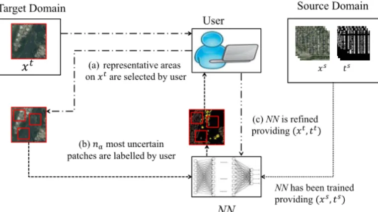
Fig. 3: Proposed active learning method depicted over three steps.NN stands for the proposed neural network,xs, ts, xt
andtt denote images and target maps over source and target
domains respectively.
The training process is summarized in Algorithm 1, where the proposed network is denoted by N N, and xs,ys and ts
denote input samples, network outputs and target maps over the training set (source domain) respectively. rwJ denotes
network parameters gradients with respect to cost function, is the momentum used in optimization and ntrain is the
number of training epochs. Notice that in practice, the training is carried out over mini-batches of samples, however in order to avoid unnecessary complexity, the mini-batches are not shown in Algorithm 1.
VI. DOMAINADAPTATIONSTRATEGIES
In this section we propose two domain adaptation strategies to improve the performance of a trained network when applied to a specific image to be segmented. The two strategies differ mainly in the required inputs, the first requiring no human intervention.
A. Batch Normalization Statistics Refinement
Algorithm 2 Batch Normalization Statistics Refinement Note: N N is first trained according to Alg. 1
1: fore= 1...nref ine do . refining overnref ine epochs 2: forn= 1...nmb do 3: {un...m+n} N N({xtn...m+n}) .forward pass 4: µ n= 1 m Pm
i=1un+i .n-th mini-batch mean
5: 2 n= 1 m Pm i=1(un+i µn) 2 . n-th mini-b. var. 6: z n {µ n[ 2 n} .n-th mini-batch statistics 7: zn=↵zn 1+ (1 ↵)zn .refining statistics The first domain adaptation strategy we propose consists in refining the BN statistics learned during training over each image to be segmented. As introduced in Sec. III, BN speeds up the training by normalizing the inputs to each layer activation function throughout a network. Borrowing the notation from [41], let the vectoru= (u(1), ..., u(d))represent
the inputs of a layer activation function. The normalized inputs are computed as:
ˆ
u(k)= u
(k) E[u(k)]
p
Var[u(k)] (3)
where E[u(k)] and Var[u(k)] are computed over each
mini-batch of train data. Since the procedure is the same for every activation function (any k), for brevity in the following we omit k e.g. replacing u(k) with u. Next, to prevent the
activation functions operating exclusively in their saturated region, the normalized inputs are shifted and scaled as
v= ˆu+ (4)
where and are learned independently for each layer. During training, BN keeps track of computed statistics (i.e. mean and variance), then such stored statistics are used to normalize the activations inputs during evaluation. Letz(n 1)
be the statistics tracked at the end of then 1-th mini-batch;
at the n-th mini-batch they are updated as
z(n)=↵z(n 1)+ (1 ↵)zn, (5) where z n are the statistics computed during the n-th mini-batch and ↵is the momentum.
Under some assumption, the statistics computed at training time can be used to normalize the activation function inputs at deployment time. However, when the network is deployed over data whose statistics do not match those of the training samples, the statistics computed at training time may be useless towards normalizing the activation function inputs. Therefore, we propose an improved BN strategy where after the network is trained, the computed statistics z are prelim-inary refined over (a subset of) the image to be segmented. Algorithm 2 details the proposed BN statistics refinement. First, the proposed network is required to be trained over source domain according to Algorithm 1. Next, for every image on target domain (xt), the trained network is refined
without requiring any annotations. Such refinement is carried out for nref ineepochs over patches extracted from the image
on target domain. After patches are split into nmb
mini-batches with length m, in each iteration a mini-batch of
patches ({xtn...m+n}) is input to the trained network so that
the activation functions inputs can be obtained ({un...m+n})
throughout the network. Next, the mean and variance of the activations are computed over the mini-batch (µn,
2 n) in order to update and refine BN layer statistics according to (5) whereZ nis the new observed statistics overn-th mini-batch,
andZn 1is the previously updated statistics. As a result, after nref ine epochs, BN layers statistics are refined according to
statistics of patches over the target domain. In our experiments, we found that the network performance is maximum when the BN statistics are updated for about 10 epochs (nref ine= 10)
with momentum↵= 0.9, independently over each test image.
Further refining the BN statistics has the effect of overfitting to the image area used for updating the statistics, jeopardizing the network performance over the rest of the image.
We would like to point out that this strategy does not require additional image labeling over target domain, since BN statistics refinement is carried out without computing loss function and without performing back-propagation as shown in Algorithm 2.
B. Active Learning
The second domain adaptation strategy we propose relies on active learning [17], [43], [18]. In this strategy, a number of patches from each image on test set (target domain) are first hand-selected and annotated by user and then are used to refine a network previously trained on training images (source domain). The strategy is divided into three steps and is illustrated in Fig. 3 and detailed in Algorithm 3.
The first step a) deals with the selection of suitable regions over the test image. Since a satellite image usually covers a large geographical area (e.g. a city and the rural surroundings), land usage classes are not distributed evenly across each image. For example, over an image, some areas may contain just buildings, whereas other areas may contain just vegetation. Furthermore, each land usage class statistics may be affected by some internal variance (e.g. buildings in some areas of a city may not look like other buildings in other areas of the same city). Therefore, during step a) the user manually locates image areas that are both representative of the different land use classes and account for at least some of each class internal variance.
During step b), at first, an uncertainty metric is computed for each patch which is extracted over representative areas during the previous step. For example, considering a binary segmentation problem of building-background, the uncertainty of thek-th patch is computed asuck=Pi1 |yk,i,1 yk,i,2|,
whereyk,i,j is the pretrained network score for the j-th class
of the i-th pixle of the k-th patch. Metricuck indicates how
much the network is uncertain about the classification of the
k-th patch. Patches over which the network is more uncertain
about the pixel classes, are in fact more useful for active learning [10]. Thus, the top-napatches with higher uncertainty
are selected to be hand-annotated by the user, for example using a graphical tool for image segmentation.
Finally, during step c), the network is refined over the
na patches labelled by the user. The refinement consists in
further optimizing the network parameters over the hand-labeled patches (xt, tt) according to the training procedure
defined in Sec. V-B. Therefore, the network can be optimized over a set of informative samples on the test image itself, finally closing the semantic gap between training and test samples.
In our experiments, the refinement employs a more conser-vative learning rate of 10 4 and only for 30 epochs. Due to
the relatively small number of annotated patches, high learning rates or long trainings may leads to overfitting to the selected patches, jeopardizing the ability of the refined network to generalize well over the rest of the test image. Note that in the first domain adaptation method, only BN statistics are refined which does not require annotations over the test image, however in the second approach, network parameters along
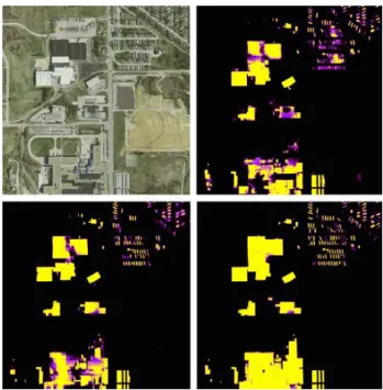
Fig. 4: Results over test area 6 in Bloomington city of INRIA dataset. The RGB input image is on the left. Score maps (Decoder SoftMax outputs) for the proposed network with 50, 101 and 152 layers follow. As the encoder depth increases, the quality of the score maps improves.
with BN statistics are both optimized providing labels over test image.
Algorithm 3 Active Learning
Note:N N is first trained according to Alg. 1
Step(a): Selecting representative areas overxtand
extract-ing patches 1: {xt
1...n} U SER(xt)
Step(b): Selecting most uncertain patches 2: {yt
1...n} N N({xt1...n}) . forward pass 3: {uc1...n} {yt1...n} . computing uncertainty 4: {xt
1...na} sort({uc1...n}) . na uncertain patches Step(c): Labellingna patches and refining N N
5: {tt} U SER({xt
1...na}) . labelling patches 6: fore= 1...nref inedo . refining overnref ine epochs
7: yt N N(xt) . forward pass 8: L(w, yt, tt) (yt, tt) . computing loss 9: J(w, yt, tt) =⌘L(w, yt, tt) + R(w). computi. cost 10: rwJ(w, yt, tt) J(w, yt, tt) . backward pass 11: ve= ve 1+rwJ(w, yt, tt) . momentum 12: we=we 1 ve . parameters optimization
VII. EXPERIMENTS ANDRESULTS
In this section, we evaluate our proposed architecture over two public and one homegrown datasets of high-resolution satellite images.
Whenever possible, we compare our results with state-of-the-art references using the appropriate metrics:
• Precision is defined as the ratio of correctly predicted
class, P recision = tp+f ptp where tp and f p are true positive and false positive pixels respectively.
• Recall is defined as the ratio of correctly predicted
pixels to all pixels that belongs to a segmentation class,
Recall= tp+f ntp wheretp,f nare true positive and false negative pixels respectively.
• F1-score is defined as the harmonic mean of precision
and recall (F1 = 2·(precision·recall)/(precision+
recall)). F1-score considers both precision and recall,
hence this metric takes both false positives and false neg-atives into account which makes it an explicit indicator of the segmentation performance.
• Intersection over Union (IoU) is the ratio of correctly
predicted area to the union of predicted pixels and the ground truth for each class IoU= tp+f p+f ntp .
• Overall accuracy is the fraction of correctly labeled pixels
for all classes, Acc=
Pnc i=1tpi
np wherenc andnp are the number of classes and the number of pixels respectively andtpi denotes true positive for classi.
The experimental setup used for all the experiments below consists of a 12-cores Intel server with 128 GB of CPU memory and four NVIDIA GeForce GTX 1080 Ti GPUs with 11 GB of memory each.
The interested readers will find more information about the implementation in the GitHib repository 1 where all codes
necessary to generate the presented results have been made publicly available.
A. Buildings dataset
The first dataset we consider for our experiments is com-posed of nine high resolution images acquired by three differ-ent Earth observation satellites over nine differdiffer-ent urban areas worldwide. The nominal spatial resolution of the images is 50 centimeters and each image includes 4 bands: red, green, blue and near infrared. Areas (cities) B1, B2, B3, B4, B5 and B6 have been chosen for training and validation, whereas areas (cities) B7, B8 and B9 are reserved for testing. That is, the network is tested over cities that are different from the cities used for training, which introduces a particularly challenging covariate shift scenario. Training and validation samples are generated as described in Section V-A, reserving 70% of areas B1, B2, B3, B4, B5 and B6 for training and the rest for validation. For each area, the ground truth includes the two classes of building and background. Thus, the problem of segmenting such dataset is a binary pixel classification problem.
1) Generalization Ability: In the first experiment, we evalu-ate the performance of our proposed architecture as a function of the encoder depth. Table II (top) shows that performance increases with the residual encoder depth. The network with the 34-layers encoder outperforms the 18-layers counterpart by 1.93% and 0.39% respectively. As the inner architecture of the residual units is identical (see Tab. I), we attribute such gain to the 16 extra residual layers. The proposed network with 152-layers encoder outperforms instead the 18-152-layers counterpart
1https://github.com/sinaghassemi/semanticSegmentation
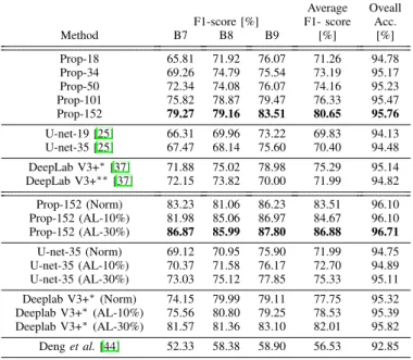
TABLE II: F1-score and accuracy over the buildings dataset test areas. Top: The proposed network and U-net with different encoder depths and Deeplab V3+ with two different backbone, Bottom: Adapted networks using BN statistics refinement (Norm), active learning over 10% 10%) and 30% (AL-30%) of each test area.
Average Oveall F1-score [%] F1- score Acc.
Method B7 B8 B9 [%] [%] Prop-18 65.81 71.92 76.07 71.26 94.78 Prop-34 69.26 74.79 75.54 73.19 95.17 Prop-50 72.34 74.08 76.07 74.16 95.23 Prop-101 75.82 78.87 79.47 76.33 95.47 Prop-152 79.27 79.16 83.51 80.65 95.76 U-net-19 [25] 66.31 69.96 73.22 69.83 94.13 U-net-35 [25] 67.47 68.14 75.60 70.40 94.48 DeepLab V3+⇤[37] 71.88 75.02 78.98 75.29 95.14 DeepLab V3+⇤⇤[37] 72.15 73.82 70.00 71.99 94.82 Prop-152 (Norm) 83.23 81.06 86.23 83.51 96.10 Prop-152 (AL-10%) 81.98 85.06 86.97 84.67 96.10 Prop-152 (AL-30%) 86.87 85.99 87.80 86.88 96.71 U-net-35 (Norm) 69.12 70.95 75.90 71.99 94.75 U-net-35 (AL-10%) 70.37 71.58 76.17 72.70 94.89 U-net-35 (AL-30%) 73.03 75.12 77.85 75.33 95.11 Deeplab V3+⇤(Norm) 74.15 79.99 79.11 77.75 95.32 Deeplab V3+⇤(AL-10%) 75.56 80.80 79.25 78.53 95.39 Deeplab V3+⇤(AL-30%) 81.57 81.36 83.10 82.01 95.82 Denget al.[44] 52.33 58.38 58.90 56.53 92.85 ⇤with ResNet101 backbone
⇤⇤with Xception backbone
by about 9% and 1% respectively. As the number of filters in each residual unit increases in blocks 2 to 4, we attribute such gain both to the four-fold increase in number of filters per layer and to the 134 extra layers. This result is in line with those of [22], where a ResNet performance in an image classification task was found to increase with its depth. As a reference, we implemented an encoder according to the plain convolutional U-Net architecture [25] with depths of 19 and 35 layers (i.e. the decoder is untouched). The two resulting networks were trained from scratch according to the procedure described in [25]. Table II (top) shows that the 18 and 34 layers residual encoder outperforms the plain convolutional encoder for similar depths of 19 and 35 layers by 1.4 % and 2.8 % respectively in terms of average F1-score. Moreover, the 18 layers residual encoder outperforms the 35 layers U-Net plain convolutional counterpart on the average. Similar results were found in [22], where a 18 layers residual network outperformed a plain 34 layers CNN in an image classification task. Such results suggest that a shallower residual encoder offers better generalization ability than a deeper plain convolutional architecture. Our experience with deep residual networks also suggests they are easier to train than plain convolutional networks, so we hypothesize that careful refinement of the U-Net optimization algorithms parameters may reduce at least in part such gap. We conclude that a deep residual encoder has better generalization ability than a shallower residual counterpart (and to some extent of a deeper plain convolutional encoder). We hypothesize that such advantage comes from the larger number of filters a
deep encoder can learn at training time that allows it to learn visual representations of high semantic level, contributing to generalization over wider range of satellite images.
In addition to U-Net, we compare with Deeplab V3+ [37], which achieved state-of-the-art performance over PASCAL VOC 2012 [45] and Cityscapes [46] datasets. Deeplab V3+ has an encoder-decoder architecture which makes use of a backbone network in the encoder for extracting feature maps. Deeplab V3+ with ResNet-101 and Xception backbones obtained the best performance in [47], therefore, we also train Deeplab V3+ once with ResNet-101 and another time with Xception backbone over building dataset. As Table II (top) shows, Deeplab V3+ with ResNet-101 backbone achieves better performance compared with Xception backbone. These results are in line with our previous findings and suggest that ResNet has better generalization ability. Nevertheless, our proposed architecture with the same depth (Prop-101) outperforms Deeplab V3+ with ResNet-101 backbone. We conjecture such gain is first related to the larger number of skip connections employed in our architecture which results in finer segmentation maps, and secondly to the deconvolutional layers used in our architecture which can be optimized during training comparing with the bilinear upsampling layers used in Deeplab V3+ decoder which have fixed filters parameters.
2) Domain Adaptation: In the second experiment, we as-sess the domain adaptation techniques proposed in Sec. VI. As a baseline, we refer to the architecture with the 152-layers encoder that achieved top performance in the previ-ous experiment. Considering the scheme in Sec. VI-A, we update the batch normalization statistics over each test image independently. In detail, we applied the procedure provided in Algorithm 2 over the trained network of Prop-152 for 10 epochs (nref ine = 10) and momentum of 0.9 (↵ = 0.9).
Table II (bottom) shows that the proposed strategy improves the network performance by about 3% over the baseline in terms of average F1-score and without the need for human input. Considering the scheme in Sec. VI-B, we independently refine the trained network over 10% 10%) or 30% (AL-30%) of each test image. Such adaptation is carried out using the procedure detailed in Algorithm 3 such that 30 epochs used for refinement (nref ine= 30) with leaning rate of 10 4
(⌘ = 10 4) and weight decay of 10 5 ( = 10 5). The
number of patches (na) used to adapt the network over test
images of B7 , B8 and B9 is 25, 20 and 20 for AL-10%, and 75, 60 and 60 for AL-30% respectively. Table II shows that the networks refined over 10% and 30% brings F1-score gains of 4% and 6% respectively over the baseline (about 1% and 3% over batch normalization statistics update).
Moreover, we also apply our proposed adaptation methods with the same parameters to the 35-layers U-Net (U-Net-35) and Deeplab V3+ with ResNet-101 backbone. As seen in Table II (bottom), U-Net-35 average F1-score improves by 1.6%, 2.3% and 4.9%, whereas Deeplab V3 average F1-score in-creases by 2.4%, 3.2% and 6.7% using BN statistics refinement (Norm) and active learning (AL-10%, AL-30%) respectively. These results imply that the proposed adaptation techniques are not specific to our architecture and other deep learning schemes can benefit from such adaptations. Nevertheless, since
our proposed architecture exhibits better generalization ability, it outperforms the other schemes in terms of segmentation peformance.
Additionally, we have implemented the active transfer learn-ing network proposed in [44] for hyperspectral images, and applied it to our 4-bands building dataset. Authors in [44] addressed the related problem of domain adaptation over satellite images by proposing a spectral-spatial feature learning network. The network include three sparse stacked autoen-coders (SSAE): one operating on extended morphological attribute profiles (spatial SSAE), another one operating on spectrum (spectral SSAE) and the last one is used to fuse the features learned using spatial and spectral SSAEs. SSAEs are trained first unsupervisedly over training samples, then based on a query criterion, a set of samples along with the labels are used to iteratively train the last softmax layer and also to fine-tune the SSAEs. As Table II shows the results of our implementation of [44] over building datasets, it can be seen that our approach outperforms it by great margin. However it should be noted that the method in [44] is originally proposed for hypersepctral images which cover very small geographical areas; conversely, our datasets include vast geographical areas and contains only 4 spectral bands.
Finally, we compare the complexity of training the proposed network (152-layers encoder) from scratch with that of adapt-ing a previously trained network. Trainadapt-ing the network from scratch for 300 epochs required 37 hours in our experimental setup. Adapting the trained network with the strategy in Sec. VI-B required 5 minutes, without accounting for the time required to annotate the area of test image used for network refinement. Otherwise, updating the batch normal-ization statistics in Sec. VI-A required about 200 seconds (no extra annotations required). Concluding, adapting a previously trained network is significantly less complex than retraining a network from scratch, offering a remarkable edge in time-critical applications such as emergency mapping.
B. INRIA Aerial Image Labeling Dataset
The second dataset we consider for our experiments is the INRIA Aerial Image Labeling Dataset [48]. Such dataset covers dissimilar urban settlements, ranging from urban areas (e.g., San Francisco’s financial district) to alpine towns with a nominal resolution of 0.3 meters. The training set consists of 180 tiles of 5000 ⇥5000 pixels from the cities of Austin, Chicago, Kitsap County, Western Tyrol and Vienna. The test set includes the same number of identically sized tiles cov-ering the cities of Bellingham, Bloomington, Innsbruck, San Francisco and Eastern Tyrol. As in the previous experiment, the network is tested over cities different from those used for training. The training set is annotated labeling each pixel as building or background; conversely, test images annotations are retained by the benchmark provider. We subdivide the annotated images into training and validation sets according to the benchmark organizer suggestions, i.e. for each city the first five tiles are reserved for validation and the rest are used for training. We retrain the network from scratch following the same procedures used for the previous experiment.
TABLE III: F1-score and Accuracy of the proposed architec-ture over INRIA validation areas as a function of the encoder depth.
F1-score [%] Average Overall
Enc. Kitsap West F1-score Acc.
Depth Austin Chicago County Tyrol Vienna [%] [%] 18 93.58 88.77 83.41 92.00 91.82 89.91 94.88 34 93.66 88.95 84.93 92.82 92.01 90.47 95.02 50 93.82 89.59 85.23 93.04 91.85 90.70 95.12 101 93.92 89.92 85.27 94.68 92.61 91.28 95.37 152 94.61 89.82 87.36 94.75 93.39 91.98 95.62
TABLE IV: Segmentation performance as IoU and Accuracy over INRIA test images (numbers provided by the benchmark organizer). IoU [%] Bellingham Bloomington Innsbruck San Francisco East Tyrol Average Overall IoU Acc. [%] [%] AMLL [49] 67.14 65.43 72.27 75.72 74.67 72.55 95.91 NUS [49] 70.74 66.06 73.17 73.57 76.06 72.45 95.90 ONERA [49] 68.92 68.12 71.87 71.17 74.75 71.02 95.63 Raisa [49] 68.73 60.83 70.07 70.64 74.76 69.57 95.30 INRIA [48] 56.11 50.40 61.03 61.38 62.51 59.31 93.93 Proposed-18 69.70 66.70 72.16 65.85 73.91 68.50 95.40 Proposed-50 68.17 67.97 73.07 66.78 75.42 69.20 95.52 Proposed-152 69.13 70.30 72.51 69.64 75.31 70.76 95.54 Prop-152 (Norm) 69.47 75.17 75.90 72.76 76.89 73.63 96.10
As a first experiment, we evaluate the performance of our proposed architecture as a function of the encoder depth. Since for this dataset no ground truth is provided for the test set, the performance is first evaluated on the validation set using 5 different encoder depths (18, 34, 50, 101, 152). Table III shows that as the encoder depth increases, the segmentation quality improves, confirming our previous findings in Table II with the buildings dataset. While validation and training sets are drawn from the same cities, we argue that the network shall be able to learn features relative to multiple cities, thus the network shall still be able to generalize across different areas of the same city.
In the second experiment, we investigate how the encoder depth and the proposed batch normalization statistics refine-ment affect the network performance over test images. For this experiment, we used the previously trained networks with 18, 50 and 152 layers encoders to segment the 5 test images. Then, only for the 152-layers network, we applied the adaptation strategy in Section VI-A to segment the 5 test images (due to the lack of the annotations required for refinement, we could not evaluate the domain adaptation strategy in Section VI-B). The BN statistics refinement is carried out following the procedure detailed in Algorithm 2 and for 10 epochs (nepochs = 10) over each image with
momentum of 0.9 (↵= 0.9). Then, the resulting segmentation
maps were provided to the benchmark organizer that computed and returned us the relative segmentation accuracy in terms of Intersection over Union (IoU) as shown in Table IV together with the top-5 performing references reported in [49].
Consistently with our previous experiments over the build-ings dataset, the results show that a deeper encoder improves the network performance over most test images. Namely, the
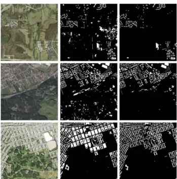
Fig. 5: In the left column, RGB images from INRIA test set are provided. Each of these images shows an area in the cities of Bloomington (top), Innsbruck (middle) and San Francisco (bottom). The central column shows the segmentation maps predicted by the proposed network (152 layers encoder). The right column shows the segmentation maps predicted by the adapted network using normalization statistics refinement over each test image.
TABLE V: F1-score and accuracy of the proposed architecture over Vaihingen validation images as a function of the encoder depth.
F1-score [%] Overall
Encoder Imp. Low Acc.
Depth Sur. Building Veg. Tree Car Avg. [%] 18 85.96 91.15 72.63 83.99 68.01 80.34 83.83 34 86.01 91.80 73.27 84.30 67.98 80.67 84.15 50 86.70 92.30 74.76 84.86 71.36 81.99 84.99 101 87.24 93.65 74.31 84.71 82.82 84.57 85.56 152 89.17 93.78 77.08 85.54 83.84 85.88 86.77
152-layers encoder network achieves a 2.26 % gain over the 18-layers encoder network in terms of average IoU and a 0.14 % gain in overall accuracy. This gain supports our finding that a deep residual encoder is able to learn visual representations that are more robust to covariate shifts, results in better performance over unseen images. Fig. 4 shows how the output score map over an area of Bloomington city from test set improves as encoder depth increases.
Finally, BN statistics refinement considerably improves by 2.87% in terms of average IoU over our baseline, outperform-ing the other references in 4 out of 6 cities and all other references both in terms of mean IoU and overall accuracy. Fig. 5 illustrates the improvement due to batch normalization statistics refinement over three images of INRIA test set.
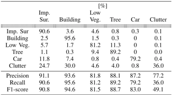
TABLE VI: Confusion matrix (top half) and segmentation performance (bottom half) for our proposed architecture with 152-layers encoder over the Vaihingen test images (numbers provided by the benchmark organizer).
[%]
Imp. Low
Sur. Building Veg. Tree Car Clutter
Imp. Sur 90.6 3.6 4.6 0.8 0.3 0.1 Building 2.5 95.6 1.5 0.3 0 0.1 Low Veg. 5.7 1.7 81.2 11.3 0 0.1 Tree 1.1 0.3 9.4 89.2 0 0.0 Car 11.8 7.4 0.8 0.4 79.2 0.4 Clutter 24.7 30.0 4.6 4.0 0.8 36.0 Precision 91.1 93.6 81.8 88.1 87.2 77.2 Recall 90.6 95.6 81.2 89.2 79.2 36.0 F1-score 90.8 94.6 81.5 88.7 83.0 49.1
TABLE VII: Segmentation accuracy over the 17 Vaihingen dataset test images (numbers provided by the benchmark organizer).
F1-score [%] Overall
Imp. Low Acc.
Sur. Building Veg. Tree Car [%] Pa.et al.[50] 89.5 93.2 82.3 88.2 63.3 88.0 Ka.et al.[3] 92.1 95.3 83.9 91.0 83.6 89.2 Au.et al.[5] 91.0 94.5 84.4 89.9 77.8 89.8 GSN [51] 91.8 95.0 83.7 89.7 81.9 90.1 DLR-9 [6] 92.4 95.2 83.9 89.9 81.2 90.3 Proposed-152 90.8 94.6 81.5 88.7 83.0 89.0
C. Vaihingen ISPRS 2D Semantic Labeling Dataset
The third and last dataset we consider for our experiments is the ISPRS 2D Semantic Labeling Dataset [52], which includes 33 areas extracted from the city of Vaihingen, Germany. Each area consists of a true orthophoto (TOP) image (near infrared, red and green bands) and relative Digital Surface Model (DSM); the ground sampling distance is 9 cm. A total of 16 areas out of 33 are meant for training and validation and are annotated with ground truth. The remaining 17 areas are meant for testing and so the related ground truth is not made available by the benchmark organizer.
While in the two previous datasets training and test images are captured from different satellites across multiple cities, with this dataset all images account for the same city as captured by the same satellite. Therefore, the covariate shift between training and test sets is small compared with the other datasets. However, while two previous datasets address a binary building-background segmentation problem, this dataset classifies each pixel into six classes: impervious surfaces, building, low vegetation, tree, car and clutter (background). Thus, whereas this dataset is less suitable to stress a network generalization ability, the presence of similar classes such as low vegetation and trees and the difficulty in distinguishing small objects such as cars from background clutter makes it a challenging test for our architecture. Moreover, this dataset includes DSM which our network is not designed to handle.
The training and validation samples are generated subdi-viding the 16 annotated areas into validation and training
subsets. Following the approach of [3] and [4], we reserve areas (11, 15, 28, 30, 34) for validation, whereas the rest is used for training. Most of the previous studies carried out on this dataset process the DSM separately and then the results are fused with those of TOP files in reason of the different nature of DSM data. However, since our goal is not to devise a scheme specialized for DSM images, we consider the DSM data as an additional color band for a total of four input bands. As for the other datasets, all networks are retrained from scratch following the same procedure.
As first experiment, we study the effect of the encoder depth on the network performance over the validation areas as the ground truth of the test areas is not available to us. Table V shows that the segmentation quality improves with the encoder depth, coherently with our previous results (the clutter class was excluded from the table following the example of the dataset provider as it is of limited interest). We observe that beside the low vegetation that can be possibly mistaken with trees, cars represent the most difficult objects to recognize, we hypothesize due to the small scale of vehicles.
As a second experiment, we use the 152-layers encoder network to segment the 17 test areas (Figure 6 shows an ex-ample of the resulting segment maps). The segmentation maps were provided to the benchmark organizer who computed the performance indices against the retained ground truth. Table VI contains the confusion matrix (top half) and per-class precision, recall and F1-score averaged over the 11 test areas (bottom half). The matrix supports our hypothesis that low vegetation can be easily mistaken with trees and shows that cars are often mistaken by impervious surfaces, which are characterized by similar small scale. Yet, our architecture is capable of correctly identifying buildings with a F1-score close to 95%.
Table VII compares our proposed architecture with the top-5 best performing references made available on the bench-mark organizer website. The DLR-9 [6] scheme achieves top performance via a network operating on three different scales. Moreover, two distinct networks are employed, one for detecting class boundaries and the other one to predict score maps. Then, the boundaries and segmentation results are fused to generate the final segment map. Audeber et al. [5] proposes similar strategy, deploying a scale and multi-modal architecture to address the pixel-based classification. Kampffmeyer et al. [3] also devised multi-modal strategy using patch-based and fully convolutional networks and also median frequency balancing is implemented on loss function to overcome the issue of unbalanced classes in dataset. By comparison, our architecture is considerably less complex since it relies on a single scale network and is not designed to deal with DSM data. Despite our architecture being simpler and meant to improve generalization, still it performs almost as well as specialized and more complex ones. For this dataset we do not report any result concerning the adaptation strategies in Sec. VI since train and test samples are captured from the same city by the same satellite, thus covariate shift is minimal.
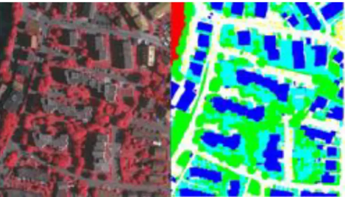
Fig. 6: Segmentation results over one test area of the Vaihingen test set for the 152-layers encoder network.
VIII. CONCLUSIONS
In this work, we designed an encoder-decoder convolu-tional network for satellite image segmentation deployable over images different from those used from training. Our experiments revealed that residual encoders offer better gener-alization abilities than a plain convolutional counterpart, and that generalization ability improves with the encoder depth. We hypothesize that deep residual architectures with a large number of filters spanning across a wider range of semantic levels allow the encoder to learn more robust features to co-variate shift. Our experiments show that refining a previously trained network significantly improves its performance with a complexity that is a fraction of that required to train a network from scratch. Interestingly, nearly 50% of such gain stems from just updating the batch normalization statistics alone, without refining the network parameters. Finally, the proposed architecture outperformed multiple references over two datasets characterized by large differences between train and test images.
ACKNOWLEDGMENTS
This work was done at the Joint Open Lab Cognitive Computing and was supported by a fellowship from TIM. We would like thank Constantin Sandu, Fabio Giulio Tonolo and Piero Boccardo from Department of Regional and Urban Studies and Planning in Politecnico di Torino for providing us the building dataset.
The Vaihingen data set was provided by the German Soci-ety for Photogrammetry, Remote Sensing and Geoinforma-tion (DGPF) [52]: http://www.ifp.uni-stuttgart.de/dgpf/DKEP-Allg.html.
REFERENCES
[1] Alex Krizhevsky, Ilya Sutskever, and Geoffrey E Hinton, “Imagenet classification with deep convolutional neural networks,” inAdvances in Neural Information Processing Systems, 2012, pp. 1097–1105. [2] Yann LeCun, L´eon Bottou, Yoshua Bengio, and Patrick Haffner,
“Gradient-based learning applied to document recognition,”Proceedings of the IEEE, vol. 86, no. 11, pp. 2278–2324, 1998.
[3] Michael Kampffmeyer, Arnt-Borre Salberg, and Robert Jenssen, “Se-mantic segmentation of small objects and modeling of uncertainty in urban remote sensing images using deep convolutional neural networks,” inProceedings of the IEEE conference on Computer Vision and Pattern Recognition Workshops, 2016, pp. 1–9.
[4] Michele Volpi and Devis Tuia, “Dense semantic labeling of sub-decimeter resolution images with convolutional neural networks,”IEEE Transactions on Geoscience and Remote Sensing, vol. 55, no. 2, pp. 881–893, 2017.
[5] Nicolas Audebert, Bertrand Le Saux, and S´ebastien Lef`evre, “Semantic segmentation of earth observation data using multimodal and multi-scale deep networks,” in Asian Conference on Computer Vision. Springer, 2016, pp. 180–196.
[6] Dimitrios Marmanis, Konrad Schindler, Jan Dirk Wegner, Silvano Gal-liani, Mihai Datcu, and Uwe Stilla, “Classification with an edge: Im-proving semantic image segmentation with boundary detection,”ISPRS Journal of Photogrammetry and Remote Sensing, vol. 135, pp. 158–172, 2018.
[7] Xiwen Yao, Junwei Han, Gong Cheng, Xueming Qian, and Lei Guo, “Semantic annotation of high-resolution satellite images via weakly supervised learning,” IEEE Transactions on Geoscience and Remote Sensing, vol. 54, no. 6, pp. 3660–3671, 2016.
[8] Sakrapee Paisitkriangkrai, Jamie Sherrah, Pranam Janney, and Anton van den Hengel, “Semantic labeling of aerial and satellite imagery,” IEEE Journal of Selected Topics in Applied Earth Observations and Remote Sensing, vol. 9, no. 7, pp. 2868–2881, 2016.
[9] Masashi Sugiyama, Neil D Lawrence, Anton Schwaighofer, et al., Dataset shift in machine learning, The MIT Press, 2017.
[10] Devis Tuia, Claudio Persello, and Lorenzo Bruzzone, “Domain adapta-tion for the classificaadapta-tion of remote sensing data: An overview of recent advances,”IEEE Geoscience and Remote Sensing Magazine, vol. 4, no. 2, pp. 41–57, 2016.
[11] Lorenzo Bruzzone and Claudio Persello, “A novel approach to the selec-tion of spatially invariant features for the classificaselec-tion of hyperspectral images with improved generalization capability,”IEEE Transactions on Geoscience and Remote Sensing, vol. 47, no. 9, pp. 3180–3191, 2009. [12] Claudio Persello and Lorenzo Bruzzone, “Kernel-based
domain-invariant feature selection in hyperspectral images for transfer learning,” IEEE Transactions on Geoscience and Remote Sensing, vol. 54, no. 5, pp. 2615–2626, 2016.
[13] Shilpa Inamdar, Francesca Bovolo, Lorenzo Bruzzone, and Subhasis Chaudhuri, “Multidimensional probability density function matching for preprocessing of multitemporal remote sensing images,” IEEE Transactions on Geoscience and Remote Sensing, vol. 46, no. 4, pp. 1243–1252, 2008.
[14] Allan A Nielsen and Morton J Canty, “Kernel principal component and maximum autocorrelation factor analyses for change detection,” inImage and Signal Processing for Remote Sensing XV. International Society for Optics and Photonics, 2009, vol. 7477, p. 74770T. [15] Giona Matasci, Michele Volpi, Mikhail Kanevski, Lorenzo Bruzzone,
and Devis Tuia, “Semisupervised transfer component analysis for domain adaptation in remote sensing image classification,” IEEE Transactions on Geoscience and Remote Sensing, vol. 53, no. 7, pp. 3550–3564, 2015.
[16] Hsiuhan Lexie Yang and Melba M Crawford, “Spectral and spatial proximity-based manifold alignment for multitemporal hyperspectral image classification,” IEEE Transactions on Geoscience and Remote Sensing, vol. 54, no. 1, pp. 51–64, 2016.
[17] Suju Rajan, Joydeep Ghosh, and Melba M Crawford, “An active learning approach to hyperspectral data classification,” IEEE Transactions on Geoscience and Remote Sensing, vol. 46, no. 4, pp. 1231–1242, 2008. [18] Giona Matasci, Devis Tuia, and Mikhail Kanevski, “Svm-based boosting
of active learning strategies for efficient domain adaptation,” IEEE Journal of Selected Topics in Applied Earth Observations and Remote Sensing, vol. 5, no. 5, pp. 1335–1343, 2012.
[19] Ian Goodfellow, Jean Pouget-Abadie, Mehdi Mirza, Bing Xu, David Warde-Farley, Sherjil Ozair, Aaron Courville, and Yoshua Bengio, “Gen-erative adversarial nets,” inAdvances in Neural Information Processing Systems, 2014, pp. 2672–2680.
[20] Yaroslav Ganin, Evgeniya Ustinova, Hana Ajakan, Pascal Germain, Hugo Larochelle, Franc¸ois Laviolette, Mario Marchand, and Victor Lempitsky, “Domain-adversarial training of neural networks,” The Journal of Machine Learning Research, vol. 17, no. 1, pp. 2096–2030, 2016.
[21] Ahmed Elshamli, Graham W Taylor, Aaron Berg, and Shawki Areibi, “Domain adaptation using representation learning for the classification of remote sensing images,”IEEE Journal of Selected Topics in Applied Earth Observations and Remote Sensing, vol. 10, no. 9, pp. 4198–4209, 2017.
[22] Kaiming He, Xiangyu Zhang, Shaoqing Ren, and Jian Sun, “Deep residual learning for image recognition,” inProceedings of the IEEE