Models and optimal designs for conjoint choice experiments including a no-choice option.

(1)

Models and optimal designs for conjoint choice experiments

including a no-choice option

Bart Vermeulen, Peter Goos and Martina Vandebroek

DEPARTMENT OF DECISION SCIENCES AND INFORMATION MANAGEMENT (KBI)

Faculty of Economics and Applied Economics

(2)

Models and optimal designs for conjoint choice

experiments including a no-choice option

Bart Vermeulen

1

Faculteit Economische en Toegepaste Economische Wetenschappen

Katholieke Universiteit Leuven

Peter Goos

Faculteit Toegepaste Economische Wetenschappen

Universiteit Antwerpen

Martina Vandebroek

Faculteit Economische en Toegepaste Economische Wetenschappen Universitair Centrum voor Statistiek

Katholieke Universiteit Leuven

Abstract

In a classical conjoint choice experiment, respondents choose one profile from each choice set that has to be evaluated. However, in real life the respondent does not always make a choice: often he/she does not prefer any of the alternatives offered. Therefore, including a no-choice option in a choice set makes a conjoint choice experiment more realistic. In the literature three different models are used to analyze the results of a conjoint choice experiment with a choice option: the choice multinomial logit model, the extended no-choice multinomial logit model and the nested no-no-choice multinomial logit model. We develop optimal designs for each of these models using the D-optimality criterion and the modified Fedorov algorithm. We compare the optimal designs with a reference design that was constructed ignoring the no-choice option and we discuss the impact of the different designs and models on the precision of estimation and the predictive accuracy based on a simulation study.

Keywords: Bayesian optimal design, choice based conjoint, conjoint analysis, D-optimality, multinomial logit model, nested logit

1

(3)

1. Introduction

The aim of a conjoint choice experiment is to model respondents’ choices as a function of the features of a product or service. In this type of experiment the respondent repeatedly chooses the alternative offering the maximum amount of utility from a number of choice sets each containing several alternatives. These experiments gain popularity for modelling market demand because of their ability to simulate market decisions realistically and because of the opportunity to estimate the impact of product or service features on market demand.

In a classical conjoint choice experiment, the respondent is forced to choose one profile from each choice set. However, in real life the customer does not always make a choice: often he/she does not like any of the alternatives presented and does not buy any of the products or services offered. Therefore, including a no-choice option in a choice set makes the experiment more realistic.

To conduct an efficient conjoint choice experiment with a small number of choice sets an optimal design has to be developed by choosing the appropriate alternatives and grouping them in choice sets in the best possible way. We examine whether an optimal no-choice design, i.e. a design constructed taking into account the presence of a no-choice option in the choice sets of the experiment, leads to better results in terms of the accuracy of the estimated model coefficients and the predicted probabilities compared to a reference design developed ignoring this no-choice option.

In the next section we discuss the respondents’ motivation to choose this no-choice option and the advantage and disadvantage of including a no-choice option in a choice set. In Section 3, three models for analyzing the data from a conjoint choice experiment with a no-choice option are discussed: the no-no-choice multinomial logit model (NCMNL), the extended no-choice multinomial logit (ENCMNL) model and the nested no-choice multinomial logit model (NLMNL). In Section 4 we explain some basic notions of experimental design and introduce the D-optimality criterion, which we apply to the NCMNL, ENCMNL and NLMNL models respectively to develop optimal no-choice and reference design. The relative performances of the reference design and the optimal no-choice designs under different scenarios are compared in Section 5. In Section 6, we use a simulation study to measure the accuracy of the parameter estimates by the expected mean squared error of the parameter estimates and the prediction accuracy of the designs by the expected mean squared error of the predicted probabilities. Finally, in Section 7 we take a detailed look at the accuracy of the predictions based on a simulation study in which the data consists of a mixture of choices generated by the three models.

(4)

2. The no-choice option

In this section we discuss several aspects of the no-choice option described in the literature. First of all we focus on the reasons why this option is attractive to respondents. Subsequently we discuss the advantage and disadvantage of incorporating this option in the design and model.

In the literature that deals with the no-choice option in choice experiments, two reasons why a respondent would choose the no-choice option can be found. According to the rationale theory, which reduces decision making to the concept of utility, the consumer prefers the product that offers him the maximum amount of utility. None of the alternatives is considered as attractive when none of them offers the respondent sufficient utility. In that case, the benefits of continuing the respondent’s search for better alternatives are larger than the costs. That is why the respondent chooses the no-choice option and looks for more useful alternatives. Psychological research provides another theory as to why a consumer chooses not to choose. The theory focuses strongly on avoiding intricate trade-offs and the related discomfort and fear of making the wrong choice. Baron and Ritov (1994), for example, state that consumers prefer bearing the consequences of inaction rather than those of wrong action. This is the reason why a consumer prefers deferring his purchase over buying the wrong product or service when he/she feels uncomfortable choosing. In this situation the no-choice option is used as a way to avoid a no-choice conflict between two alternatives with nearly equal utilities. Johnson and Orme (1996), however, found no evidence for such a behaviour and claim that respondents tend not to choose the no-choice option to avoid difficult decision making.

In this article, we therefore assume that the respondents determine the utility for each option and choose the no-choice option if none of the alternatives offers sufficient utility. Consequently the meaning of the no-choice option given in this paper is “None of the alternatives meet my requirements” meaning the customer prefers to continue to look for better alternatives. The rationale theory enables us to use the multinomial model which is the focus of the following sections (Dhar (1997) and Dhar and Simonson (2003)).

The major advantage of including a no-choice option in a conjoint choice experiment is that a more realistic experiment is obtained. The experiment therefore leads to better estimates of the model parameters and to better predictions of market penetrations. As a matter of fact, forcing a respondent to make a choice in a conjoint choice experiment might lead to biased parameters when analyzing the choice data (Dhar (1997) and Dhar and Simonson (2003)). That including a no-choice option in the experiment avoids the bias is a major advantage which should outweigh the disadvantage that, each time a respondent selects the no-choice

(5)

option, no information is collected concerning the relative attractiveness of the alternatives offered.

3. Multinomial logit models

In this section, we discuss the multinomial logit model and the nested multinomial logit model. For each of these models, we first review the logit probability of choosing an alternative and the likelihood function of the corresponding model. Within the class of multinomial logit models, Haaijer, Kamakura and Wedel (2001) describe two models for analyzing data from choice experiments that have a no-choice option: the NCMNL model and ENCMNL model. The use of these two models, described in Section 3.1, requires the “independence of irrelevant alternatives” assumption to be valid. The violation of this assumption necessitates the use of the nested logit model which is the subject of Section 3.2. In this paper, we refer to the nested logit model as the NLMNL model.

3.1 The NCMNL and ENCMNL model

The most popular model to analyze choice data is the multinomial logit model. If a respondent n faces choice set k with J alternatives, then the utility of alternative j experienced by respondent n can be expressed as

'

nkj kj nkj

u

=

x

β ε

+

. (1)

The p-dimensional parameter vector β represents the importance of the attributes for the consumer in determining his/her utility. We assume that this vector is common for all respondents. The vector xkj has the same dimension as β and contains the levels of the

attributes of the product or service represented by the jth alternative in choice set k. The error term εnkj captures the influence of unobserved factors on the utility experienced by the

respondent. All error terms are assumed to be independent and identically extreme value distributed. Under this assumption, the probability that respondent n chooses alternative j of choice set k is

( )

∑

=

_J i ki kj nkj

x

P

1 ' '

exp

β

. (2)

If we assume that N respondents evaluate the same set of K choice sets, the log-likelihood function for the multinomial logit model becomes

. (3)

( )

(

)

∑∑∑

(

= = =

=

N n K k J j nkj nkj

P

y

L

1 1 1

ln

β

)

The dummy variable ynkj equals one when respondent n prefers alternative j of choice set k

and zero otherwise. The maximum likelihood estimate βˆ for the parameter vector is obtained by maximizing the log-likelihood function.

(6)

Like Haaijer, Kamakura and Wedel (2001), we distinguish two multinomial logit models for analyzing choice experiments with a no-choice option. The simplest model, the NCMNL model, represents the no-choice option by including an alternative having zero values for all attribute levels. Consequently the utility of the no-choice option in the NCMNL model is always zero. This method of coding creates an extra level for each attribute in the study which possibly leads to distorted parameter estimates.

In the second model, the ENCMNL model, an extra no-choice dummy variable is used to represent the choice option. This offers the advantage of an enhanced model fit. The no-choice dummy variable acts as an additional two-level attribute and takes value zero for all real-choice options and value one for the no-choice option. The model parameter corresponding to the dummy variable is interpreted as the utility of choosing the no-choice option by the respondent. As the primary interest of researchers is not in the estimation of that model parameter, we develop optimal designs that focus on the precise estimation of the other model parameters, i.e. the part-worths of the original attributes.

A problem with both the NCMNL and the ENCMNL models is that they require the strong assumption of the independence of irrelevant alternatives, commonly referred to as the IIA-assumption, to be valid. Under this IIA-assumption, the relative odds of choosing alternative j over j’ depend only on the attributes of j and j’ no matter what the attributes of the other alternatives are. This implies that the unobserved parts of the utilities of the alternatives exhibit no correlation. While the IIA-assumption is a realistic one in some choice situations, it is not appropriate in others where it can lead to biased estimators and consequently to incorrect predictions (Train, 2003). Now, it turns out that the IIA-assumption is often violated when some of the alternatives in a choice set are more similar than others. This is exactly what happens in choice sets that have a no-choice option because there is a group of real options and one totally different option, the no-choice option. A nested logit model can therefore be used in such situations.

3.2 The nested no-choice multinomial logit model (NLMNL)

In case the IIA-assumption is violated, the family of generalized extreme value models offers alternative ways to analyze the choice data. The most widely used model in this family is the nested multinomial logit model in which the probability of choosing alternative j of nest m in choice set k is modelled as

Pjkm = P(m)P(j|m), (4) where

( )

(

)

(

)

1 exp exp m m M i i i V P m V λ λ = =

∑

,

(5)

(7)

( )

∑

=

m J i ki kj

x

m

j

P

1 ' '

exp

β

(6) and

( )

⎟⎟

⎠

⎞

⎜⎜

⎝

⎛

=

∑

= m J i ki m

x

V

1 '

exp

ln

β

.

(7)

In these expressions, P(m) denotes the likelihood that nest m is chosen from a set of M nests,

P(j|m) is the conditional probability that alternative j is chosen out of the Jm alternatives in nest

m given that nest m was chosen, Vm is the so-called inclusive value of nest m and λm is the

dissimilarity coefficient corresponding to nest m. The inclusive value Vm is interpreted as the

expected utility a respondent experiences from choosing nest m. The dissimilarity coefficients

λm usually lies between 0 and 1 and measures to what extent the alternatives in nest m are

different (for a detailed discussion, see Börsch-Supan (1990)). Values for λm close to zero

therefore indicate that the alternatives in nest m are very similar and that the use of nesting is justified. A λm value of one indicates that the alternatives in nest m are so different that

grouping them in a nest is not useful.

The parameter vector β can be estimated by the standard maximum likelihood method. The log-likelihood function for the nested logit model can be written as

( )

(

)

∑∑∑∑

(

= = = =

=

N n K k M m J j jkm njkm m

P

y

L

1 1 1 1

ln

β

)

(8)

Maximizing this likelihood function to find the maximum likelihood estimates is hard because of its potential non-concavity (Train, 2003). This necessitated us to use different starting values for the parameters and to repeat the optimisation procedure for each of them to obtain the maximum likelihood estimates.

For accommodating the no-choice option in the nested logit model, we follow the work of Haaijer, Kamakura and Wedel (2001), who suggested using one nest containing the no-choice option and another nest containing the real-no-choice options. The no-no-choice option is represented using zero values for all attributes. We refer to the resulting model as the NLMNL model. The rationale behind this model is a two-stage decision process. First, the respondent either selects the nest containing the real-choice options or the nest containing the no-choice option. In the former case, the second stage in the decision process consists of the respondent choosing one of the alternatives from the nest with real choices.

4. Constructing D-optimal designs for no-choice models

In this section, we introduce the D-optimality criterion and discuss the problem of constructing an optimal design for non-linear models such as the NCMNL model, the ENCMNL model and

(8)

the NLMNL model considered here. Also, we explain how we constructed a reference design for evaluating the D-optimal designs for each of these models.

4.1 Constructing D-optimal designs for a conjoint choice experiment

The aim of a conjoint choice experiment is to model how the respondents’ choices depend on the attributes of products and services. To achieve this goal in an efficient way, the experiment can be designed so that its information content is maximized somehow. The resulting experimental design is then said to be optimal. Finding an optimal design for a conjoint choice experiment involves selecting the alternatives to be presented to the respondents and arranging these alternatives in choice sets according to some optimality criterion. The literature on the optimal design of experiments distinguishes several criteria to select a designed experiment. The criteria that received attention in the marketing literature are the D-, A-, G- and V-optimality criteria (see, e.g., Huber and Zwerina (1996), Sándor and Wedel (2001) and Kessels, Goos and Vandebroek (2006a)). The most widely used of these is the D-optimality criterion which offers the advantage that the relative performance of different experimental designs with respect to it is independent of the coding strategy or scale used (Goos (2002)).

In general, D-optimal designs maximize the determinant of the Fisher information matrix on the unknown parameters contained within the vector β and thereby minimize the volume of the confidence ellipsoid around β. As the Fisher information matrix is inversely proportional to the variance-covariance matrix of the parameter estimates, a D-optimal design is also said to minimize the generalized variance of the parameter estimates.

The performance of a design in terms of the D-optimality criterion is expressed by the D-error

(

)

{

}

1

{

(

)

}

1

det , p det ,

D= I X

β

− = V X

β

p_{, (9)}

where I(X,β) denotes the Fisher information matrix, V(X,β) is the variance-covariance matrix and the matrix X contains the attribute levels for all the alternatives in the experiment. The conjoint choice design having the smallest D-error is called the D-optimal design.

Because of the nonlinearity of the NCMNL, ENCMNL and NLMNL models, the D-error not just depends on the matrix X but also on the unknown model parameters contained within the

β vector. As a result of that, prior knowledge of the model parameters is required to develop an optimal design for the three models. However, this knowledge is not available when the experiment is planned. The three approaches adopted in the literature on the optimal design of conjoint choice experiments for circumventing this problem are reviewed by Kessels, Goos and Vandebroek (2006a). In one approach, zero prior values are assumed for all parameters in β to simplify the optimal design problem and to obtain theoretical results (see, e.g., Burgess

(9)

and Street, (2003, 2005), Schwabe et al. (2003) and Grasshoff et al. (2004)). The assumption of zero prior values is however strong as it comes down to assuming that the respondents are indifferent between all levels of all attributes. Huber and Zwerina (1996) presented a second approach to handle the dependence on the unknown parameters. They suggested non-zero prior parameter values obtained from small-sample pretests or managers’ prior beliefs. The resulting optimal designs are referred to as locally optimal designs in the optimal design literature and lead to more precise parameter estimates and predictions than designs developed based on zero prior parameter values provided these prior values are sufficiently close to the true values. A third approach for dealing with the problem of the model’s nonlinearity is the Bayesian optimal design approach introduced in the marketing literature by Sándor and Wedel (2001). In this approach a prior distribution of possible parameter values is used instead of a single guess based on pretests or managers’ beliefs. When there is substantial uncertainty about the unknown parameters, the Bayesian optimal designs outperform the locally optimal design in terms of the D-error.

We use the Bayesian approach assuming a prior distribution f(β) on the parameters. The Bayesian version of the D-error is denoted by Db-error and defined as the expected value of

the D-error over this prior distribution:

(

)

{

det ,

}

1

{

det ,

(

)

}

1 ( ) . p p b i i p D E_β I X β − V X β f β d ℜ ⎡ ⎤ = ⎢ ⎥= ⎢ ⎥ ⎣ ⎦

∫

β (10)

Because there is no analytical expression for this quantity, it is usually approximated by taking a large number of draws from the prior distribution and averaging the D-error over all draws. If we denote the draws by β1, β 2, …, βR with R the number of draws, the Db-error is calculated as

(

)

{

}

{

(

)

}

1 1 1 1 1 1 det , det , . R R p p b i i i D I X V X R β R − = = =

∑

=

∑

β_i

)

(11)

The conjoint design that minimizes this Db-error is the Bayesian D-optimal design. To seek for

a D-optimal design, we used the modified Fedorov algorithm introduced in Kessels, Goos and Vandebroek (2006a). This heuristic algorithm seeks optimal designs by exchanging profiles of a random start design by profiles from a candidate set. Several random starting designs were used to avoid local optima and the best design found over the different random starts is considered the Db-optimal design.

4.2 Optimal designs for the NCMNL and ENCMNL models

When either the NCMNL or the ENCMNL model is used, the Fisher information matrix I(X,β) for a given β can be written as

(

)

'

(

' 1

,

K i i i i i i

I X

β

N

X P

p p

=

∑

−

X

(12)

(10)

(Huber and Zwerina, 1996), where Xi is the part of X containing the attribute levels of the

profiles in choice set i, pi is a vector in which the jth element represents the probability that

the jth profile is chosen in choice set i and Pi is a diagonal matrix with on the main diagonal

the values of pi. We use expression (11) which approximates the Db-error to find an optimal

no-choice design for the NCMNL model and for the ENCMNL model. Note that the number of rows in every Xi equals the number of real-choice alternatives plus one for the no-choice

option in every choice set. For the ENCMNL, every Xi also has an extra column because of

the dummy variable that is used for the no-choice option in that model. As a result of that, the dimension of the information matrix I(X,β) for the ENCMNL model is equal to p+1 when p

denotes the number of model parameter corresponding to the attributes under investigation.

The designs we computed for the ENCMNL model were constructed such that they were D

-optimal for the p parameters corresponding to the attributes under investigation. This is because the primary interest of researchers is in gathering information on the magnitudes of these parameters. In the literature on the optimal design of experiments, designs that are D -optimal for a subset of parameters are called a Ds-optimal designs (see, e.g., Atkinson and

Donev (1992)).

4.3 Optimal design for the NLMNL model

Goos, Vandebroek and Vermeulen (2007) show that the information matrix about the unknown parameters β and λ in the nested no-choice multinomial logit model is equal to

(13)

(

)

,

'

,

⎥

⎦

⎤

⎢

⎣

⎡

=

c

X

DX

X

N

X

I

π

λ

β

where the matrix D, the vector π and the constant c are all rather complicated functions of the probabilities λ, Pjkm(j,m), P(m) and P(j|m)

.

As the interest of the researcher mainly is in

estimating β, they prefer minimizing the generalized variance of the estimate of β. As a result, a Ds-optimal design is needed here too. Finding it requires the maximization of det(X’DX-c -1_X’_ππ_’X

) instead of det(I(X,β,λ)). This is also done in a Bayesian fashion in this article.

4.4 Reference design

The estimation and prediction performances of the D-optimal designs for the NCMNL,

ENCMNL and NLMNL models will be compared to a D-optimal design for a multinomial model that does not accommodate a no-choice option. In the sequel of this paper, the latter design will serve as a benchmark and will be referred to as the reference design. We have chosen the D-optimal design for the multinomial logit model as a reference design because, in terms of precision of estimation, it is the best alternative design option currently available in the literature on the design of conjoint choice experiments.

(11)

In the following sections we investigate how well the reference design described earlier performs relative to the optimal designs for the NCMNL, ENCMNL and NLMNL models when estimating these models and when using them to make predictions. The criteria we used to compare the four design options are the Db-error, the estimation precision and the accuracy of

the predicted probabilities of choosing alternatives in different choice sets.

5. Design comparisons in terms of Db-error

In this section, we compare the reference design and the optimal designs based on the Db

-error. The results we report are for choice designs with 16 choice sets consisting of two real-choice alternatives and a no-real-choice option. Each real-real-choice option is described by two attributes having three levels and one attribute having two levels. Other number of choice sets, attributes and attribute levels produced similar results to the ones reported here.

5.1 Computational aspects

In our calculations, we used effects-type coding for the attribute levels. For three-level attributes, the first, second and third level are then represented by the vectors [1,0], [0,1] and [-1,-1], respectively. For two-level attributes, the values 1 and -1 are associated with the first and second level, respectively. Effects-type coding is illustrated in Table 1, where the coding of the no-choice option in each the three models considered in this paper is also shown. Notice that, in the ENCMNL, a dummy variable is used for the no-choice option.

Attribute levels of the choice set

Coding for NCMNL

and NLMNL Coding for ENCMNL

Level attr. 1

Level attr. 2

Level

attr. 3 Attr. 1 attr. 2 attr. 3 attr. 1 attr. 2 attr. 3

no -choice dummy 3 1 2 -1 -1 1 0 -1 -1 -1 1 0 -1 0 2 3 1 0 1 -1 -1 1 0 1 -1 -1 1 0 No-choice option 0 0 0 0 0 0 0 0 0 0 1

Table 1: Effects-type coding for the NCMNL, ENCMNL and NLMNL models.

As explained in Section 4.1, calculating Bayesian D-optimal designs requires the specification of a prior distribution for the model parameters β and λ. The resulted presented in this paper were obtained assuming the prior parameters drawn from a p-variate normal distribution with mean [-0.5 0 -0.5 0 -0.5] and variance 0.5*Ip, where Ip is the p-dimensional identity matrix.

This prior distribution is in agreement with the recommendations formulated in Kessels,

Jones, Goos and Vandebroek (2006b). To calculate the Db-errors for the NCMNL and

ENCMNL models and for computing the reference design, we used 1000 draws from the normal prior distribution for each parameter of the model in order to approximate the Bayesian design criteria. For the ENCMNL model, a prior distribution was also needed for the

(12)

coefficient of the extra dummy variable. We used a normal distribution with mean -0.5 and variance 0.5 for that, and we utilized 1000 draws from that distribution for calculating the Db

-error for designs for that model. For the NLMNL model however, we used 250 draws only because its complicated information matrix slowed down the design construction algorithm, which was a modified Fedorov algorithm like the one in Kessels, Goos and Vandebroek (2006a). For the NLMNL, we also used 250 draws from the uniform distribution on the ]0;1[ interval for the parameter λ. We include in the appendix the reference design and the optimal no-choice designs for the three models with 16 choice sets of three profiles.

5.2 Comparison of design options in terms of Db-error

In this section, we compare the Db-errors for the reference design and the optimal no-choice

designs for the NCMNL, ENCMNL and NLMNL models. For that purpose, we have calculated one Db-error for every combination of a design and a no-choice model. This does not only

allow us to evaluate how much better it is to take into account the no-choice option when designing the choice experiments, but it also enables us to look at the robustness of the different designs when the model used to analyze the data is not the model used to construct the design. The 12 Db-errors are displayed in Table 2. The numbers in bold correspond to

scenarios for which the model used for generating the design was the same as the one used for analyzing the data.

Model used to design the choice experiment Model used to

analyze data MNL NCMNL ENCMNL NLMNL

NCMNL 0.2643 0.2578 0.2588 0.2964

ENCMNL 0.2555 0.2529 0.2526 0.2895

NLMNL 0.2711 0.2591 0.2630 0.2042

Table 2:Db-errors of the Db-optimal designs constructed for the MNL model ignoring the

no-choice option and the NCMNL, ENCMNL and NLMNL models which do take into account the no-choice option.

It turns out that the reference design and the optimal designs for the NCMNL model and the ENCMNL model perform almost equally well for fitting a multinomial logit model with a no-choice option. These designs however perform poorly for fitting the NLMNL model compared to the optimal design for this model. The reverse is also true: the optimal design for the NLMNL model leads to poor Db-errors when used to fit the NCMNL and ENCMNL models.

(13)

6. Evaluating the performance of the optimal no-choice designs

In this section we report the results of a simulation study to examine the accuracy of the estimated coefficients and the predicted probabilities for choosing an alternative.

6.1 Criteria for evaluation

In order to examine the accuracy of the estimated coefficients we use the expected mean squared error

( )

(

) (

) ( )

ˆ

k

EMSE

_β

β

β β

f

β

d

β

ˆ

ℜ

′

=

∫

−

, (13)

where

f

( )

β

ˆ

is the distribution of the estimated parameters and

β

ˆ

and

β

are vectors containing the estimated and the true parameter values respectively. Evidently, small

ˆ

EMSE

_β values are preferred over large ones. In our computations, we approximated the

ˆ

EMSE

_β value by performing a large number of simulations for each set of parameters β and taking the average squared difference between

β

ˆ

and

β

over all simulations. Denoting the number of simulations by R, the

EMSE

_β_ˆ values reported in this article are thus computed as

( )

(

) (

ˆ 1

1

R

ˆ

r r r

EMSE

R

β

)

=

′

=

∑

−

. (14)

We used R = 1000 in our simulations and computed

EMSE

_βˆ values for 60 draws of the

parameters β coming from a p-variate normal distribution with mean [-0.5 0 -0.5 0 -0.5] and variance 0.5*Ip. Values for the coefficient of the no-choice dummy variable in the ENCMNL

and for λ in the NLMNL were again drawn from a normal distribution with mean -0.5 and variance 0.5 and from the uniform distribution on the interval ]0;1[. In the next sections, the 60

EMSE

_β_ˆ values for different scenarios are reported in side-by-side box-plots.

To assess the accuracy of the predictions obtained from the estimated models, we also calculated the expected mean squared error of the predicted probabilities, EMSE_p_ˆ. This measure compares the probabilities obtained from the estimated coefficients and the probabilities obtained with the real parameter values for all possible combinations of two real-choice options and the no-real-choice option. Formally, the EMSEpˆ value is defined as

( )

(

( )

)

(

( )

)

( )

ˆ

k p

ˆ

EMSE

β

p

β

p

β

p

β

p

β

f

β

d

ℜ

′

=

∫

−

β

, (15)

(14)

where the vectors

p

ˆ

( )

β

ˆ

and

p

( )

β

contain the probabilities for all possible choice sets containing two real-choice options obtained using the estimated and the real parameter values, respectively. Like for the

EMSE

_βˆ, small values for the EMSEpˆ are desired and simulations were used to approximate it:

( )

(

( )

)

'

(

( )

)

ˆ 1

1

ˆ

r r R p p p p r

EMSE

p

R

β

=

∑

−

β

_p . (16)

Here too we used R = 1000. Just like for the

EMSE

_β_ˆ, we computed EMSEpˆ values for 60 draws of the parameters under different scenarios and we report them using box-plots.

In our simulation study, we started by assuming that the NCMNL was the true model. Using that model, data for 100 respondents were generated using the four different designs, namely the reference design and the optimal designs for the three no-choice models under investigations. Next, the data generated according to the reference design were analyzed using each of the NCMNL, ENCMNL and NLMNL models. Also, the data generated according to each optimal design were analyzed using the model for which the design was constructed. This led us to study six different scenarios for each of the data-generating models and explains why each of the Figures 1 to 7 contains six box-plots. In each of these figures, the box-plots appear in pairs. The left pair of box-plots shows

EMSE

_βˆ or EMSEpˆ values obtained when analyzing the data using the NCMNL model. The middle pair of box-plot contains the results for situations in which the ENCMNL is used to analyze the data, and, finally, the right pair contains results for the NLMNL model. In each pair of box-plots, the left plot gives the results for the reference design and the right plot gives the results for the optimal design.

6.2 Choices generated by the NCMNL model

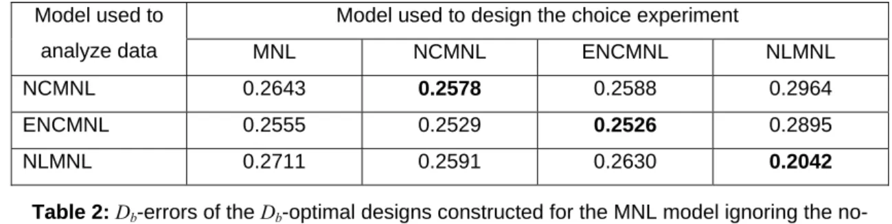
When the choices are generated by the NCMNL model, all design and analysis options perform almost equally well in estimating the parameters. This can be seen in Figure 1. It turns out that, for none of the three models, there is a significant difference in the accuracy of the estimated parameters between the reference and the optimal design. In other words, taking into account the no-choice option when constructing a choice design does not lead to a substantial gain in terms of estimation accuracy. This complements the results of Street and Burgess (2004) who concluded that designs developed for a forced choice setting can be used to include a no-choice option at the cost of a slightly reduced estimation precision when zero prior parameters values are assumed. That the reference design and the optimal designs for the NCMNL and ENCMNL models perform similarly is logical because they are based on similar non-nested multinomial logit models. The optimal design for the NLMNL model is based on a different type of model, namely a nested one, and this explains the

(15)

slightly less accurate estimated parameters in the scenario where the data are generated by a non-nested multinomial model..

Figure 1: EMSE_βˆ values when choices are generated by the NCMNL model. The left, middle and right pairs of box-plots show the EMSE_βˆ values obtained when analyzing the data using the NCMNL, ENCMNL and NLMNL model, respectively. In each pair, the left and right plots give the results for the reference design and the optimal design, respectively.

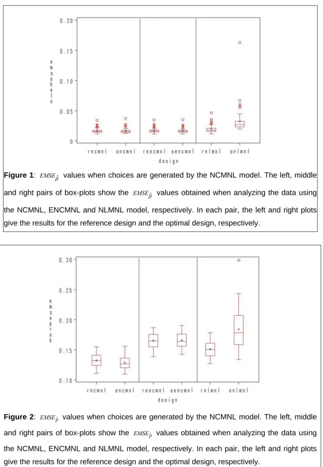
Figure 2: values when choices are generated by the NCMNL model. The left, middle

and right pairs of box-plots show the values obtained when analyzing the data using

the NCMNL, ENCMNL and NLMNL model, respectively. In each pair, the left and right plots give the results for the reference design and the optimal design, respectively.

ˆ p EMSE ˆ p EMSE

(16)

By comparing the EMSEpˆ values in the box-plots in the left panel of Figure 2 with those in the other panels, it can be seen that the choice probabilities were estimated more precisely when the data were analyzed using the NCMNL model, no matter whether the reference design or the optimal design for that model is utilized. Also when the data are analyzed using the ENCMNL model, whether or not the optimal design is used makes no substantial difference. There is however a clear difference between the two design options when the NLMNL model is used for analyzing the data generated by the NCMNL model. That the difference is in favour of the reference design is because that design was optimized for a non-nested multinomial logit model, which is similar to the model used for generating the data.

6.3 Choices generated by the ENCMNL model

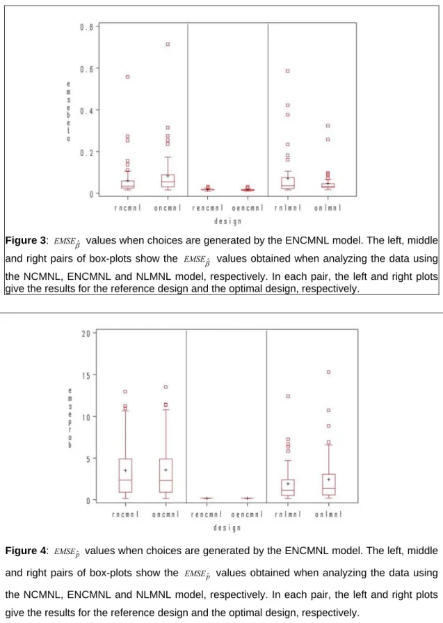
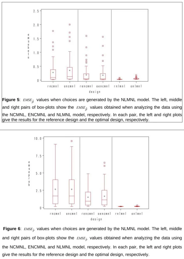
When the choices are generated by the ENCMNL model, the conclusions are very similar to the situation in which the data were produced by means of the NCMNL model. This can be seen from Figures 3 and 4, in which the box-plots for the

EMSE

_β_ˆ and EMSEpˆ values are displayed. Again, there is no significant difference between the reference design and the optimal designs in terms of the accuracy of the estimated parameters and the predicted probabilities. However, as can be seen from the box-plots for the

EMSE

_β_ˆ values in Figure 3, analyzing the data using the ENCMNL is now substantially better than using any of the two other models. This result is true for both the reference design and the optimal design for the ENCMNL model. Notice also that the optimal design for the NLMNL performs better when the data are generated using the ENCMNL model than when using the NCMNL. This indicates that the ENCMNL model is conceptually more similar to the NLMNL model than the NCMNL model. The box-plots for the EMSEpˆ values in Figure 4 show that the predictions by means of the ENCMNL model are significantly better than those based on the other models. This result is true for the reference design as well as for the optimal design for that model.

6.4 Choices generated by NLMNL

Finally, Figures 5 and 6 visualize the accuracy of the estimated parameters and predictions when the choices are generated by the NLMNL model. To generate data using that model, we drew a random value from a uniform distribution on the interval ]0;1[ for the dissimilarity parameter λ for every draw of β. Even in the case where the data are generated using the NLMNL model, there is no substantial gain in terms of estimation accuracy and prediction accuracy from taking into account the no-choice option when designing the choice experiment. This can be seen by looking at the box-plots for the

EMSE

_β_ˆ values in Figure 5 and those for the EMSEpˆ values in Figure 6. What does matter is the model used to analyze

(17)

the data: the estimates and the predicted probabilities are far more precise when the NLMNL model is utilized for the analysis rather than the NCMNL or the ENCMNL model.

Figure 3: EMSE_βˆ values when choices are generated by the ENCMNL model. The left, middle and right pairs of box-plots show the EMSE_βˆ values obtained when analyzing the data using the NCMNL, ENCMNL and NLMNL model, respectively. In each pair, the left and right plots give the results for the reference design and the optimal design, respectively.

Figure 4: values when choices are generated by the ENCMNL model. The left, middle

The simulation results in Figures 1 to 6 show that the differences between the three models for analyzing the data are larger than the differences between the design options. None of the

(18)

models appears to lead to accurate estimates and predicted probabilities when the model selected to analyze the data does not match the model used to generate the data.

Figure 5: EMSE_βˆ values when choices are generated by the NLMNL model. The left, middle and right pairs of box-plots show the EMSE_βˆ values obtained when analyzing the data using the NCMNL, ENCMNL and NLMNL model, respectively. In each pair, the left and right plots give the results for the reference design and the optimal design, respectively.

Figure 6: values when choices are generated by the NLMNL model. The left, middle

(19)

7. Evaluating the performance of no-choice designs based on mixed responses

In the previous section we assumed that the model generating the data is the same for all respondents. In this section, we relax this assumption and investigate the situation where respondents act according to different models. For that purpose, we generate choices using each of the three models investigated in this paper. For 100 of the respondents, we used the NCMNL model to generate the responses. For another 100 respondents, the ENCMNL model was used and, for the final 100, the NLMNL model was utilized. For all 300 respondents the same choice sets -given by one of the four designs- were used. The designs used were again the reference design and the optimal designs displayed in the appendix. The data generated using the reference design were analyzed using each of the models, whereas the data generated with one of the optimal designs were only analyzed using the model for which the

designs was optimized. Box-plots of the EMSEˆp values obtained in that fashion are

displayed in Figure 7. The box-plots were constructed for 20 draws of the model parameters. The same distributions as before were used for these draws.

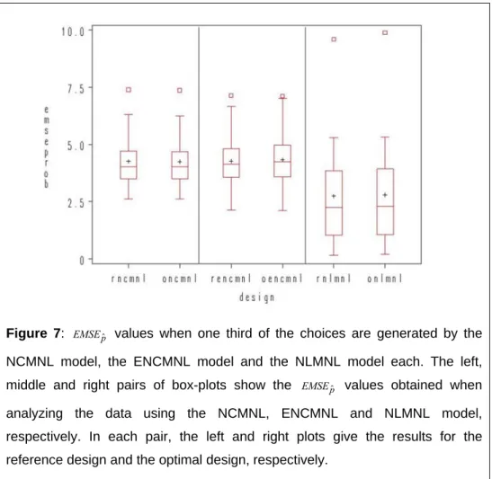
Figure 7: values when one third of the choices are generated by the NCMNL model, the ENCMNL model and the NLMNL model each. The left,

middle and right pairs of box-plots show the values obtained when

analyzing the data using the NCMNL, ENCMNL and NLMNL model, respectively. In each pair, the left and right plots give the results for the reference design and the optimal design, respectively.

(20)

Figure 7 shows that there is no substantial improvement in prediction error from including the no-choice option in the design process. Furthermore the figure reveals that the predictions obtained from the NLMNL are substantially more precise than those produced by the other models. This difference is statistically significant. Consequently, the NLMNL model is most robust in predicting the choice probabilities when the respondents’ behaviour cannot be explained using a single model.

8. Conclusion

In a classical conjoint choice experiment the respondent is forced to choose an alternative of the choice set even if none of the alternatives is valued highly. However, in reality the respondent always has the possibility to postpone his/her decision and to continue his/her search for better alternatives. Because more accurate predictions are expected from a more realistic choice experiment, it is believed that including a no-choice option in every choice set of a choice experiment leads to more accurate predictions.

In this paper, three models were considered for analyzing data from choice experiments including a no-choice option. The no-choice multinomial logit model represents the attributes of the no-choice options by means of zero values. In the extended no-choice multinomial logit model, a no-choice dummy variable is added to the model. The nested no-choice logit model divides the alternatives in a no-choice nest and a real-choice nest clustering the real-choice options of the choice set. We developed optimal designs for these models and compared them with a reference design that was constructed ignoring the fact that the experiment involved a no-choice option in every choice set. The reference design was an optimal design for a multinomial model without assuming that a no-choice option was utilized during the experiment.

The accuracy of the estimated parameters and the predicted probabilities of the optimal designs (that were constructed taking into account the presence of a no-choice option in each choice set) and the reference design (that was constructed ignoring the presence of the no-choice option) were examined by means of a simulation study. Remarkably, there was no substantial gain in terms of either estimation precision or prediction accuracy from using the optimal designs for the no-choice models compared to the reference design. An optimal design for the multinomial model, as computed in Huber and Zwerina (1996), Sándor and Wedel (2001) and Kessels, Goos and Vandebroek (2006a) can therefore be used also when a no-choice option is considered. Although we did not find differences between the different design options studied in this article, our simulation study revealed the importance of selecting the appropriate model for analyzing the data. Using the wrong model leads to less accurate estimates and predictions. In cases where there is uncertainty about which model to select, the nested multinomial logit model seems to produce the best results.

(21)

APPENDIX

I. Reference design

Choice set Profile Attr. 1 Attr. 2 Attr. 3 Choice set Profile Attr.1 Attr. 2 Attr. 3

1 1 1 1 1 2 2 1 2 2 2 1 2 1 3 2 1 3 No-choice option 9 3 No-choice option 1 3 2 2 1 1 3 1 2 2 3 1 2 2 2 2 2 3 No-choice option 10 3 No-choice option 1 1 1 2 1 1 1 2 2 3 2 1 2 2 3 1 3 3 No-choice option 11 3 No-choice option 1 1 2 2 1 2 3 2 2 2 1 1 2 3 2 1 4 3 No-choice option 12 3 No-choice option 1 1 2 1 1 2 3 1 2 2 1 2 2 1 2 1 5 3 No-choice option 13 3 No-choice option 1 2 2 1 1 2 2 2 2 3 1 2 2 3 1 1 6 3 No-choice option 14 3 No-choice option 1 1 2 2 1 3 3 1 2 3 1 2 2 2 1 2 7 3 No-choice option 15 3 No-choice option 1 3 3 2 1 1 3 2 2 2 1 2 2 3 1 2 8 3 No-choice option 16 3 No-choice option

(22)

II. Optimal design for the NCMNL model

(23)

III. Optimal design for the ENCMNL model

(24)

IV. Optimal design for the NLMNL model

(25)

References

Atkinson, A.C. and Donev, A.N. (1992), Optimum experimental designs, Oxford U.K.,

Clarendon Press

Baron, J. and Ritov, I. (1994), Reference points and omission bias, Organizational

Behavior & Human Decision Processes, 59, 475-498

Börsch-Supan, A. (1990), On the compatibility of nested logit models with utility

maximization, Journal of Econometrics, 46, 373-388.

Burgess, L. and Street, D.J. (2003), Optimal designs for 2k choice experiments,

Communications in Statistics: Theory and Methods, 32, 2185-2206.

Burgess, L. and Street, D.J. (2005), Optimal designs for choice experiments with

asymmetric attributes, Journal of Statistical Planning and Inference, 134, 288-301.

Dhar, R. (1997), Consumer preference for a no-choice option, Journal of Consumer

Research, 24, 215 – 231

Dhar, R. and Simonson, I. (2003), The effect of forced choice on choice, Journal of

Marketing Research, 40, 146-160

Goos, P. (2002), The Optimal Design of Blocked and Split-Plot Experiments, New

York, Springer

Goos, P., Vermeulen, B. and Vandebroek, M. (2007), D-optimal conjoint choice designs for a nested logit model when a no-choice option is used, Unpublished manuscript.

Grasshoff, U., Grossmann, H., Holling, H. and Schwabe, R. (2004), Optimal designs

for main-effects in linear paired comparison models, Journal of Statistical Planning

and Inference, 126, 361-376

Haaijer, R., Kamakura, W., and Wedel, M. (2001), The ‘no-choice’ alternative in

(26)

Huber, J. and Zwerina, K. (1996), The importance of utility balance in efficient choice

designs, Journal of Marketing Research, 33, 307-317

Johnson, R.M. and Orme, B.K. (1996), How many questions should you ask in choice-based conjoint studies?, Sawtooth Software Technical Paper, available at http://www.sawtoothsoftware.com/download/techpap/howmanyq.pdf

Kamakura, W.A., Kim, B-D. and Lee, J. (1996), Modeling preference and structural

heterogeneity in consumer choice, Marketing Science, 15, 152-172

Kessels, R., Goos, P. and Vandebroek, M. (2006a), A comparison of criteria to

design efficient choice experiments, Journal of Marketing Research, 43, 409-419

Kessels, R., Jones, B., Goos, P. and Vandebroek, M. (2006b), Recommendations on the use of Bayesian optimal designs for choice experiments, Research Report KBI_0617, Department of Decision Sciences and Information Management, Katholieke Universiteit Leuven, 18 pp

Sándor, Z. and Wedel, M. (2001), Designing conjoint choice experiments using manager’s prior beliefs, Journal of Marketing Research, 38, 430-444

Schwabe, R., Grasshoff, U., Grossmann, H. and Holling, H. (2003), Optimal 2K paired

comparison designs for partial profiles, in PROBASTAT2002: Proceedings of the 4th

International Conference on Mathematical Statistics, Tatra Mountains Mathematical Publications, vol. 26, edited by Stulajter, F. and Wimmer, G., 79-86.

Street, D.J. and Burgess, L. (2004), Optimal stated preference choice experiments

when all choice sets contain a specific option, Statistical Methodology 1, 37-45

Train, K. (2003), Discrete Choice Methods with Simulations, Cambridge University

Press

Zwerina, K., Huber, J. and Kuhfeld, W.F. (1996), A general method for

constructing efficient choice designs, working paper, Fuqua School of

Business, Duke University, NC 27708, Updated version available from SAS

Institute

(http://support.sas.com/techsup/technote/ts722e.pdf)

http://support.sas.com/techsup/technote/ts722e.pdf)