University of Nebraska - Lincoln
DigitalCommons@University of Nebraska - Lincoln
Dissertations & Theses in Natural Resources Natural Resources, School of
8-2018
A Comparison of VNIR and MIR Spectroscopy for
Predicting Various Soil Properties
Joshua R. Gates
University of Nebraska-Lincoln, [email protected]
Follow this and additional works at:http://digitalcommons.unl.edu/natresdiss
Part of theHydrology Commons,Natural Resources and Conservation Commons,Natural Resources Management and Policy Commons,Other Environmental Sciences Commons, and the Water Resource Management Commons
This Article is brought to you for free and open access by the Natural Resources, School of at DigitalCommons@University of Nebraska - Lincoln. It has been accepted for inclusion in Dissertations & Theses in Natural Resources by an authorized administrator of DigitalCommons@University of Nebraska - Lincoln.
Gates, Joshua R., "A Comparison of VNIR and MIR Spectroscopy for Predicting Various Soil Properties" (2018).Dissertations &
Theses in Natural Resources. 264.
A COMPARISON OF VNIR AND MIR SPECTROSCOPY FOR PREDICTING
VARIOUS SOIL PROPERTIES
by
Joshua R. Gates
A THESIS
Presented to the Faculty of
The Graduate College at the University of Nebraska
In Partial Fulfillment of Requirements
For the Degree of Master of Science
Major: Natural Resource Sciences
Under the Supervision of Professor Paul Hanson
Lincoln, Nebraska
A COMPARISON OF VNIR AND MIR SPECTROSCOPY FOR PREDICTING
VARIOUS SOIL PROPERTIES
Joshua R. Gates, M.S.
University of Nebraska, 2018
Advisor: Paul Hanson
Soil plays an important role in our daily lives, namely producing food, cleaning
water and storing carbon. The ability to rapidly and cost-effectively quantify the various
components of soils can help us understand and better manage this important resource.
This study aims to compare the ability of visible near-infrared (VNIR) spectroscopy and
mid-infrared (MIR) spectroscopy to quickly and accurately predict various important soil
properties (electrical conductivity, soil pH, cation exchange capacity, exchangeable
cations, phosphorus, carbon, beta-glucosidase enzyme activity and nitrogen). Prediction
models were developed using partial least squares regression (PLSR) techniques. Three
different calibration sampling methods were tested along with various spectral
preprocessing techniques to find the best predictive ability of VNIR and MIR. Soil
components related to carbon, nitrogen and cation exchange capacity had good predictive
ability (R2 > 0.8) by both VNIR and MIR, but MIR was more accurate. Electrical
conductivity, sodium cations and phosphorus were poorly predicted by both (<0.71).
VNIR models were not as robust as MIR models but could be potentially useful for
qualitative analyses when rapid analyses are preferred over methods are more accurate.
MIR predictions overall yielded more accurate predictions than VNIR and could
potentially be used as a surrogate method for timely laboratory techniques for spectrally
iii
Table of Contents
List of Figures ... vi
List of Tables ... vi
List of Equations ... vii
CHAPTER 1. INTRODUCTION ... 1
1.1 Purpose of Study ... 1
1.2 Objectives ... 2
CHAPTER 2. BACKGROUND & LITERATURE REVIEW ... 3
2.1 Introduction ... 3
2.2 Electromagnetic Radiation and Matter ... 4
2.3 Spectral Preprocessing ... 8
2.4 Chemometrics ... 10
2.5 Predicting Soil Properties ... 13
2.5.1 Electrical Conductivity ... 14
2.5.2 Soil pH ... 15
2.5.4 Cation Exchange Capacity and Exchangeable Cations ... 18
2.5.5 Carbon ... 19
2.5.6 β-Glucosidase ... 22
2.5.7 Nitrogen ... 22
2.6 Summary ... 23
CHAPTER 3. MATERIALS & METHODS ... 25
3.1 Study Area ... 25
3.2 Reference Data Collection ... 26
3.2.1 Air-dry Oven-dry Ratio... 26
3.2.2 Electrical Conductivity ... 26
3.2.3 Soil pH ... 27
3.2.4 Water Soluble Phosphorus ... 28
3.2.5 Cation Exchange Capacity ... 30
3.2.6 Extractable Bases ... 32
3.2.7 Calcium Carbonate... 36
3.2.9 Total Phosphorus ... 39
3.2.10 Soil Organic Carbon ... 41
iv
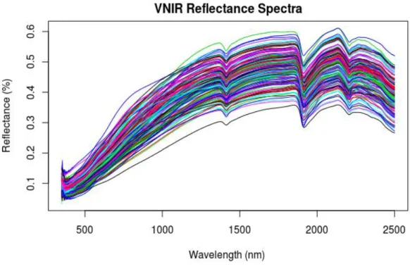
3.3 Collection of Spectra... 43
3.3.1 Vis-Near Infrared Spectroscopy ... 43
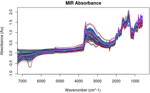
3.3.2 Mid-Infrared Spectroscopy ... 46
3.4 Statistical Analyses ... 47
3.4.1 Spectral Preprocessing ... 47
3.4.2 Model Creation and Validation ... 48
3.4.3 Model Performance and Selection ... 49
CHAPTER 4. RESULTS ... 51
4.1. Basic Soil Properties ... 51
4.1.1 Electrical Conductivity ... 57
4.1.2 Soil pH ... 57
4.1.3 Cation Exchange Capacity and Exchangeable Cations ... 59
4.1.4 Phosphorus ... 64 4.1.5 Carbon ... 66 4.1.6 β-Glucosidase ... 69 4.1.7 Nitrogen ... 70 4.2 Calibration Sampling ... 71 4.2.1 Random Sampling ... 71 4.2.2 Stratified Sampling ... 74
4.2.3 Kennard Stone Sampling ... 77
CHAPTER 5. DISCUSSION & CONCLUSION ... 79
5.1 General Soil Properties ... 79
5.1.1 Electrical Conductivity ... 79
5.1.2 Soil pH ... 80
5.1.3 Cation Exchange Capacity and Extractable Cations ... 81
5.1.4 Phosphorus ... 82 5.1.5 Carbon ... 83 5.1.6 β-Glucosidase ... 84 5.1.7 Total Nitrogen ... 84 5.2 Calibration Sampling ... 85 5.2.1 Random Sampling ... 85 5.2.2 Stratified Sampling ... 86 5.2.3 Kennard-Stone Sampling ... 86
v
REFERENCES ... 90
APPENDIX A: R CODE ... 96
APPENDIX B: SOIL REFERENCE DATA ... 112
APPENDIX C: SOIL PROPERTY CORRELATIONS ... 124
vi
List of Figures
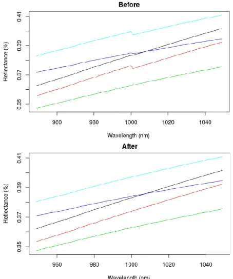
Figure 2.1 The electromagnetic spectrum (page 5) Figure 2.2 A soil absorbance spectrum (page 7) Figure 3.1 Study area and location of sites (page Figure 3.2 VNIR raw reflectance spectra (page 44) Figure 3.3 VNIR detector correction (page 45) Figure 3.4 VNIR raw absorbance spectra (46) Figure 3.5 MIR raw absorbance spectra (47)
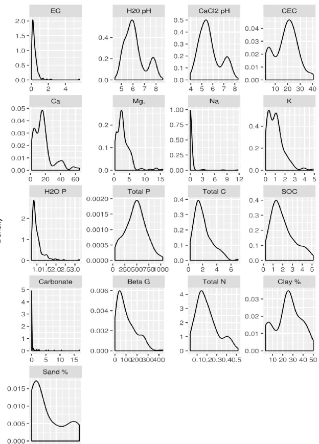
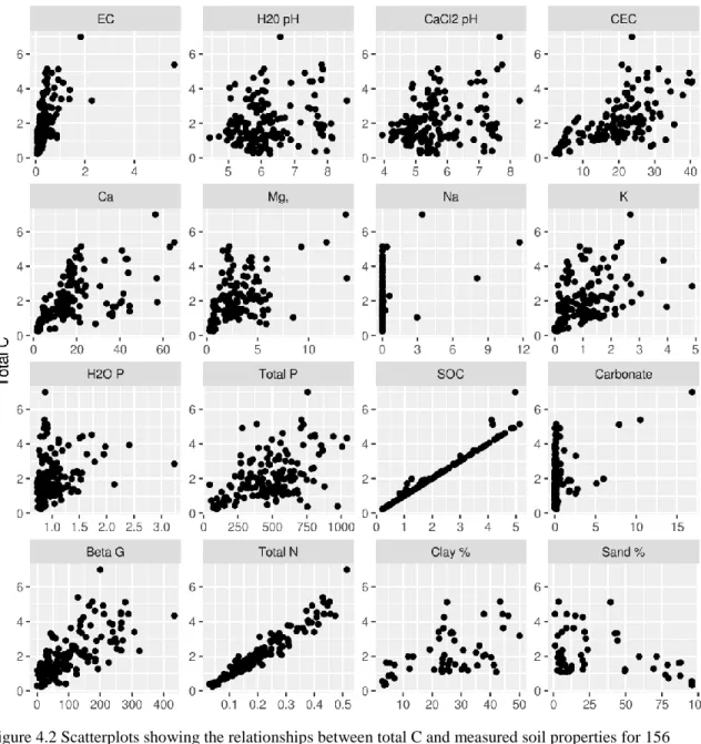
Figure 4.1 Distribution of measured soil properties (page 50)
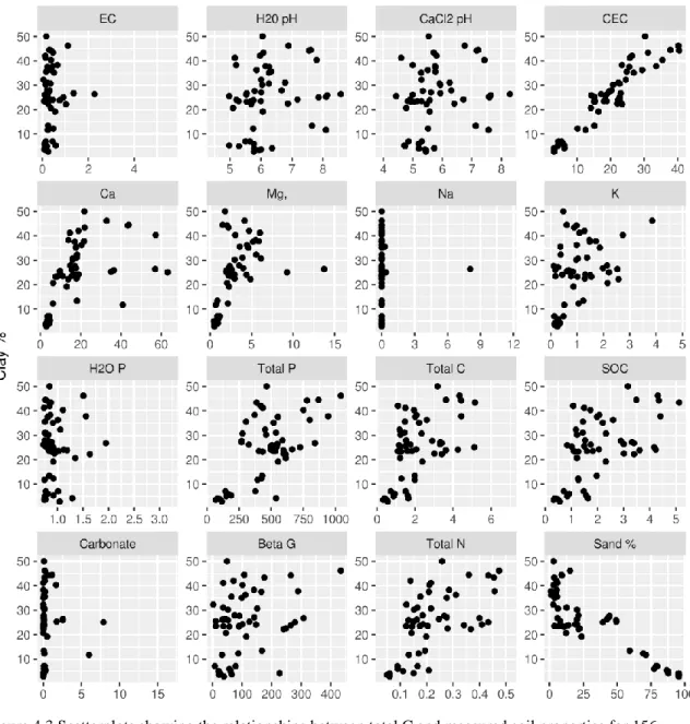
Figure 4.2 Relationship between total C and measured soil properties (page 54) Figure 4.3 Relationship between clay percent and measured soil properties (page 55) Figure 4.4 Goodness of fit plots for EC (page 57)
Figure 4.5 Goodness of fit plots for 1:1 H2O pH (page 58)
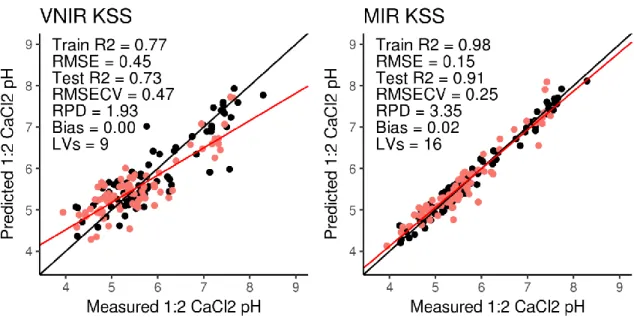
Figure 4.6 Goodness of fit plots for 1:2 CaCl2 pH (page 59)
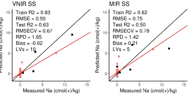
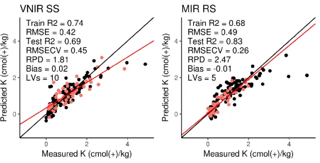
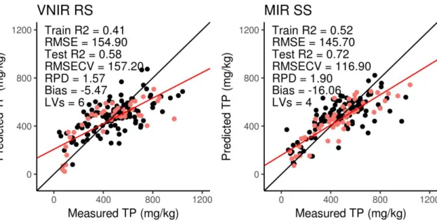
Figure 4.7 Goodness of fit plots for CEC (page 60) Figure 4.8 Goodness of fit plots for Ca (page 61) Figure 4.9 Goodness of fit plots for Mg (page 62) Figure 4.10 Goodness of fit plots for Na (page 63) Figure 4.11 Goodness of fit plots for K (page 64) Figure 4.12 Goodness of fit plots for water P (page 65) Figure 4.13 Goodness of fit plots for total P (page 66) Figure 4.14 Goodness of fit plots for total C (page 67) Figure 4.15 Goodness of fit plots for SOC (page 68) Figure 4.16 Goodness of fit plots for CaCO3 (page 69)
Figure 4.17 Goodness of fit plots for βG (page 70) Figure 4.18 Goodness of fit plots for total N (page 71)
List of Tables
Table 3.1 Qualitative model performance based on RPD and R2 (page 50) Table 4.1 Descriptive statistics of measured soil properties (page 52) Table 4.2 Correlation with spectrally active properties (page 52)
Table 4.3 Goodness of fit statistics for overall best VNIR models (page 56) Table 4.4 Goodness of fit statistics for overall best MIR models (page 56) Table 4.5 Goodness of fit statistics for VNIR with random sampling (page 73) Table 4.6 Goodness of fit statistics for MIR with random sampling (page 74) Table 4.7 Goodness of fit statistics for VNIR with stratified sampling (page 76) Table 4.8 Goodness of fit statistics for MIR with stratified sampling (page 76)
Table 4.9 Goodness of fit statistics for VNIR with Kennard Stone sampling (page 78) Table 4.10 Goodness of fit statistics for MIR with Kennard Stone sampling (page 78)
vii
List of Equations
Equation 1: Beer’s Law (page 6) Equation 2: Reflectance (page 6)
Equation 3: Reflectance to absorbance (page 6)
Equation 4: MSC correction coefficient estimation (page 8) Equation 5: MSC corrected spectrum (page 8)
Equation 6: SNV corrected spectrum (page 9)
Equation 7: Detrending 2nd order polynomial regression (page 9) Equation 8: Detrended spectra (page 9)
Equation 9: RMSEP (page 12) Equation 10: RPD (page 12)
Equation 11: AD:OD ratio (page 26)
Equation 12: Absorption to concentration (page 29) Equation 13: Extractable P conversion to soil P (page 29) Equation 14: CEC (page 32)
Equation 15: Cation concentration (page 33) Equation 16: BG activity (page 36)
Equation 17: Manometer correction (38)
Equation 18: Calcium carbonate equivalent (page 38) Equation 19: Total carbon % (page 39)
Equation 20: Total nitrogen % page (39)
Equation 21: Major element concentration (page 41) Equation 22: SOC % (page 42)
Equation 23: Reflectance to Absorbance (page 44) Equation 24: RMSECV (page 49)
Equation 25: RPD (page 49) Equation 26: Bias (page 49)
1
CHAPTER 1. INTRODUCTION
1.1 Purpose of Study
Soil is a complex and heterogeneous system with many physical, chemical, and
biological processes that govern our food and fiber production, water infiltration,
contaminant remediation and carbon sequestration. Understanding these processes can be
difficult and time-consuming. Conventional analytical techniques often ignore the
complex behaviors of soils by trying to draw relationships between physical, chemical,
and biological properties that have been analyzed and quantified independently from
subsamples and may further complicate our understanding of soils as a system by
disrupting the soil equilibrium with chemical extractions (Viscarra Rossel et al.,
2006).These techniques are often slow and expensive when cost-effective, and efficient
analytical techniques are needed to better quantify our greatest natural resource.
Spectroscopic techniques such as: mass spectroscopy (MS), nuclear magnetic
resonance (NMR), ultraviolet (UV), visible (VIS), near-infrared (NIR) and mid-infrared
(MIR), may in some cases be an alternative to traditional soil analyses (Janik et al., 1998;
Nocita et al., 2015). Great advances have been made in the last few decades to increase
the cost-effectiveness, speed, and accuracy of spectroscopic analytical methods
(Bellon-Maurel & McBratney, 2011). These methods are able to quickly analyze soil as a whole
without the need for hazardous chemicals and have the added benefit of being able to
measure multiple soil properties from a single soil sample (Viscarra Rossel et al., 2006).
Development of these techniques is crucial for our understanding of soils as a system and
2 1.2 Objectives
The main objective of this thesis is to compare the predictive ability between
VNIR and MIR spectroscopy for various soil properties at the regional scale. The soil
properties of interest are electrical conductivity (EC), pH, cation exchange capacity
(CEC) and extractable cations (Ca2+, Mg2+, Na+, K+), water-soluble phosphorus (H 2O P),
total phosphorous (P), total carbon (C), soil organic carbon (SOC), calcium carbonate
(CaCO3), β-glucosidase enzyme activity (βG), and total nitrogen (N). A variety of
spectral preprocessing techniques were tested to improve spectral signals in order to
increase model performance. Additionally, three different model calibration sampling
schemes were tested to find the best overall partial least squares regression (PLSR) model
3
CHAPTER 2. BACKGROUND & LITERATURE REVIEW
2.1 Introduction
Soil is one of the most important natural resources on Earth. It provides the
structure that allows us to produce food, fiber, and fuel that we depend on every day. Soil
provides a habitat for microbes that decompose, process and recycle nutrients; filter water
and remediate contaminants; soils can sequester carbon from carbon dioxide in the
atmosphere (Lal, 2015). Therefore, understanding these complex soil processes and
quantifying soil properties is important for ensuring our growing population has access to
fresh water and continues to produce adequate food supplies.
Assessments of soil quality require measurements of many soil parameters over
large areas to be of use in mitigating threats to soil health and in implementing
management policies. Unfortunately, analytical laboratory techniques for measuring soil
properties can vary widely between laboratories, hindering the exchange of comparable
quantitative information (Nocita et al., 2015). Traditional laboratory techniques for
analyzing soil chemical, physical and biological properties can be time-consuming, may
utilize hazardous chemicals and are destructive to the sample. Most laboratory methods
only measure one soil property at a time and therefore, it may be difficult to make
correlations on a system as heterogeneously complex as soil (Stenberg et al., 2010).
Spectroscopic techniques allow for the simultaneous characterization of various soil
constituents in a cost-effective and timely manner (Viscarra Rossel et al., 2006).
The benefits of spectroscopy are rapid, timely, cost-effective and nondestructive
analysis of soil. Soil samples are processed minimally by oven drying, grinding and
4 short period of time and the instruments are easy to use and require very little training
(Viscarra Rossel et al., 2006), allowing a tremendous amount of information to be
quickly gathered about the soil. However, spectroscopic predictions may lack the
accuracy of traditional analytical laboratory methods, especially for those properties that
are not spectrally active.
Choosing between VNIR or MIR spectrometers usually comes down to cost.
VNIR spectrometers utilize less expensive technology, are often smaller, and can be
easily accommodated in a backpack for field use (Knadel et al., 2013). However, they
tend to be less accurate and have larger prediction errors. Depending on the soil property,
this may not be acceptable for precision agricultural practices, but if the goal is to collect
large amounts of coarse data, such as environmental monitoring or assessing changes in
soil carbon content, the slight increase in accuracy gained from MIR may not be worth
the cost (Viscarra Rossel et al., 2006).
2.2 Electromagnetic Radiation and Matter
Spectroscopy is the study of how electromagnetic (EM) radiation and matter
interact. The electromagnetic (EM) spectrum is composed of the various frequencies of
electromagnetic radiation that have energy (photons) as is illustrated in figure 1. EM
radiation can be measured by its wavelength (nm or μm) or by its wavenumber (cm-1). It
is more common to use wavelength when referring to relatively short wavelengths such
as visible (400-700 nm) light or near-infrared (700-2500nm) radiation. Spectroscopists
commonly switch to wavenumbers when referring to mid-infrared (4000-400 cm-1)
radiation because it directly relates to the amount of energy of the radiation (energy
5
Figure 2.1 The electromagnetic (EM) spectrum highlighting the far infrared (FIR), thermal infrared (TIR), mid-infrared (MIR), near-infrared (NIR), red (R), green (G), blue (B), and ultraviolet (UV) regions (McBratney et al., 2003)
EM radiation interacts with matter in three ways: reflection, transmission, and
absorption. In the visible region of the spectrum, the colors you see are examples of
reflected radiation, and the colors you do not see are examples of absorbed radiation.
Molecules are composed of elements bonded together. These bonds are continuously
moving and have specific vibrational modes (stretching and bending) that occur when
exposed to visible and infrared radiation. When molecular bonds are exposed to levels of
radiation (energy) that match a bonds vibrational mode, the bond will absorb the photon,
inducing an excited vibrational state that has energy equal to the absorbed photon (Clark,
2017). The frequency (wavelength or wavenumber) at which this absorption occurs can
be used to identify and quantify specific molecules.
Absorbance cannot be directly measured but it can be calculated according to
6 decreases exponentially as the distance the light travels (path length) increases,
concentration of the absorbing substance increases, and how strongly the substance can
absorb light (extinction coefficient). More simply stated, absorbance is linearly related to
the concentration of the absorbing substance (equation 1):
(1) 𝐴 = −𝑙𝑜𝑔(𝐼0
𝐼) = 𝜀𝑙𝑐
where, A is absorbance (Au), Iois the intensity of transmitted radiation, I is the intensity
of incident radiation, ε is the extinction coefficient, l is the path length and c is the
concentration of the substance (Osibanjo et al., (2017). In soil spectroscopy, reflectance is
easier to measure than transmittance and is used as a replacement for transmittance,
where reflectance is calculated as the ratio of reflected radiation to incident radiation
(equation 2) (Bellon-Maurel and McBratney, 2011):
(2) 𝑅 =𝑅𝑜
𝑅𝐼
where, R is reflectance, Ro is the amount of radiation reflected and RI is the incident
radiation. Using Beer’s Law (equation 3), we can calculate absorbance from reflectance
(Stenberg et al., 2010):
(3) 𝐴 = 𝑙𝑜𝑔1
𝑅
Vibrational spectroscopy works according to these assumptions, that absorbance
is linearly related to the concentration of the substance, and that absorption occurs at
specific wavelengths for specific molecular bonds (Clark, 2017). Many organic
compounds have distinct absorption features in the MIR region, making MIR
spectroscopy a valuable tool. These absorption features occur at the frequency required to
excite a molecular bond or functional group to its first excited vibrational state or
7 molecule can be excited to additional vibrational states or overtones. Since energy and
frequency are proportional, the first overtone occurs at twice the wavenumber of the
fundamental vibration and absorbs approximately twice the energy (Shay and Holmes,
2015). Organic compounds in the VNIR region contain a multitude of absorption bands
related to first and second overtones, and combination bands (more than one fundamental
vibration occurring simultaneously). These absorption features tend to be broader, less
defined and more complex than the fundamental vibrational features in the MIR, making
it more difficult to accurately quantify concentrations of the absorbing substance
(BenDor et al., 1997; Zornoza et al., 2008; Bellon-Maurel and McBratney, 2011). Figure
2.2 shows an absorbance spectrum of soil.
Figure 2.2 Soil spectrum shown in the visible (VIS), near infrared (NIR) and mid-infrared (MIR).
Absorption bands of kaolinite (K), quartz (Q), smectite (S), calcite (Ca), organic compounds (OC) and soil free water (OH). Dashed lines in the bottom figure indicate the boundaries between the visible and near infrared and the near infrared and mid-infrared, respectively. (Viscarra Rossel et al., 2006).
8
2.3 Spectral Preprocessing
Variations in the spectra, often caused by the light scattering effects of quartz sand
or by instrument drift, sometimes require spectral preprocessing to improve adsorption
features by reducing the noise (Rinnan et al., 2009). Spectral preprocessing techniques
can be generally divided into three categories: scatter correction, spectral smoothing, and
spectral derivatives.
The three commonly used scatter correction techniques are; multiplicative scatter
correction (MSC), standard normal variate (SNV), and spectral detrending. MSC is one
of the most widely used preprocessing technique to increase signals by reducing the
effects of light scattering or path length (Rinnan et al., 2009). The MSC algorithm
generates new spectra in two steps, first by estimating the correction coefficients by
performing ordinary least squares regression on a spectrum (equation 4):
(4) 𝑥𝑖 = 𝑏0+ 𝑏1⋅ 𝑥𝑟𝑒𝑓+ 𝜀
where, xi is the ith uncorrected spectrum, xref is the reference spectrum obtained by taking
the average of all the spectra by wavelength, b0 and b1 are scalar parameters, and ε are the
residuals. The next step corrects the spectrum with the correction coefficients (equation
5):
(5) 𝑥𝑚𝑠𝑐 = 𝑥𝑖−𝑏0
𝑏1
where, xmsc is the ith corrected spectrum (Rinnan et al., 2009). SNV, another popular
pre-processing technique for scatter correction, has a similar form to MSC (equation 6) but
differs from MSC by operating on spectra independently. SNV is performed by centering
9 (6) 𝑥𝑠𝑛𝑣 =
𝑥𝑖−𝑎0
𝑎1
where, xsnv is the spectrum of corrected values, xiis the original spectrum, a0 is the mean
absorbance value of the spectrum and a1 is the standard deviation of the absorbance
values (Rinnan et al., 2009). Detrending removes the mean function by first fitting a 2nd
order polynomial (equation 7):
(7) 𝑥𝑖 = 𝑎𝜆2+ 𝑏𝜆 + 𝑐 + 𝑒 𝑖
where, xi is the ith spectrum; λ is the vector of wavelengths; a, b, and c are coefficients
estimated by ordinary least squares and ei are the residuals, then the detrended spectrum
is found by subtracting the mean function from the spectral response (equation 8):
(8) 𝑥𝑖∗ = 𝑥𝑖− (𝑎𝜆2+ 𝑏𝜆 + 𝑐) = 𝑒𝑖
where, 𝑥𝑖∗ is the detrended spectrum (Barnes et al., 1989).
Spectral smoothing techniques are also common and involve averaging sections
of spectra by a given gap size (Zornoza et al., 2008). Window smoothing averages the
values of each section sequentially by overlapping with the previously averaged gap. A
second type of smoothing is Savitsky-Golay (SG) smoothing which operates in the same
way as window smoothing but averages all the gaps at once and can enhance absorption
peaks (Burns and Ciurczak, 2001).
The third category of signal processing, spectral derivatives, have long been used
with other spectroscopic techniques to improve signals (Rinnan et al., 2009). A first-order
spectral derivative is obtained by finding the rate of change between points determined
by the gap size from a smoothed spectrum. A second-order derivative is then obtained by
10
2.4 Chemometrics
Quantifying soil properties from MIR and VNIR spectral data requires the use of
chemometric techniques. Chemometric techniques aim to extract relevant information
from complex systems using mathematical and statistical techniques. For prediction
purposes, techniques involve multivariate data analysis and model calibration and
validation (Geladi, 2003).
Following preprocessing of spectra, multivariate techniques such as, multiple
linear regression (MLR), principal component analysis (PCA), and partial least squares
regression (PLSR) are used to analyze spectra. MLR cannot be applied to datasets that
are collinear, such as spectra, and require the variables to be reduced, likely by band
selection. This technique loses much of the information that may have been present when
using the whole spectra (Bertrand et al., 2001).
PCA and PLSR are much better suited to handle spectra because they serve two
purposes. They both are used to convert a set of highly correlated variables to a set of
independent variables and to reduce data dimensionality by extracting the most important
variables (Geladi, 2003; Tinti et al., 2015). PCA decomposes the matrix of predictor
variables (spectra) into principal components (latent variables) that maximize the
variance among variables. These principle components are independent of each other and
can be used as new predictor variables in a regression model. PCA works well when there
are more observations than original variables (n > k) but is limited when there are more
variables than observations, as is usually the case with spectral datasets.
Much like PCA, PLSR decomposes the collinear variables into latent variables
11 (the same as in multiple linear regression). PLSR attempts to maximize both the variance
between response variables and latent variables (Wold et al., 2001). Because PLSR takes
the response variable into account, it is capable of analyzing data with fewer observations
than variables. For this reason, PLSR is more useful than PCA for building regression
models from smaller datasets (Tinti et al., 2015).
Other multivariate techniques often used for predicting soil properties from
spectral data include artificial neural networks (ANN) and regression trees (RF) and have
modeled soil properties successfully (Minasny and Mcbratney, 2008; Wijewardane et al.,
2016). While these methods are powerful if given enough input data, they can be very
complicated and often cannot explain how soil spectra and soil properties are related.
Additionally, these methods are prone to overfitting if not properly validated (Martens,
2001).
Any model created from multivariate methods must be validated in order to
determine the model’s performance, a process commonly done by splitting the data into calibration and validation sets. The calibration set is used to train the model with and the
validation set is used to test the model. If the dataset is large, this can typically be
accomplished by randomly assigning some independent subset of the data as the training
set and the rest to the test set. It is necessary to have enough observations to best describe
the relationship between the spectra and response in order to train the model, usually
done by randomly assigning two-thirds of the data to the calibration set and the remaining
third to the validation set (Estienne et al., 2001). When the number of observations is
small, a leave-one-out or jack-knifing approach may be used to increase model
12 done by training the calibration set on the whole dataset minus a subset of the data and
validating the model with the subset. This process is repeated with a new subset that is
independent of the first and is continued until every observation has been used to test the
calibration set.
The many differences in modeling techniques can make it hard to compare and
assess model performance across different studies. The coefficient of determination (R2)
can be used to compare the degree of relationship between the observed and predicted
values and is often used to test goodness of fit for calibration models. However, this
value is dependent on the range of the dataset and should not be the only criteria used for
characterizing model performance (Davies & Fearn, 2006). Reeves and Smith (2009)
considered threshold values for model performance as: very good (R2 > 0.9), useful (R2
from 0.7-0.9), and not useful (R2 < 0.7). Janik et al., (1998) suggested that models with
high correlation (R2 > 0.9) are a suitable replacement for traditional laboratory techniques
and those from 0.7-0.9 may be a useful surrogate for analysis that are time-consuming
and costly. The standard error of prediction (SEP) or root mean square error of prediction
(RMSEP) are statistical parameters commonly used to describe model prediction
performance (Estienne et al., 2001; Bellon-Maurel et al., 2010). RMSEP is computed as
the sum of squares of the differences between the predicted and the actual values for the
validation/test set (equation 9):
(9) 𝑅𝑀𝑆𝐸𝑃 = √∑ (𝑦^ −𝑦𝑖 𝑖)
2 𝑛𝑡
𝑖=1
𝑛𝑡
where nt is the number of samples in the test subset, ŷ is the predicted value and y is the
true value. The RMSEP, like R2, is affected by the range of the measured quantity and
13 (Bellon-Maurel et al., 2010). A common way this is done is to divide the standard
deviation of the response by the RMSEP (equation 10) (Davies and Fearn, 2006;
Bellon-Maurel et al., 2010). This result is the Ratio of Performance to Deviation (RPD), with
higher values indicating a better fitted model. Chang et al. (2001) defined threshold
values for model reliability as excellent (RPD > 2.0), fair (1.4 < RPD < 2), and poor
(RPD < 1.4).
(10) 𝑅𝑃𝐷 = 𝜎
√∑𝑚 (𝑦𝑖^ −𝑦𝑖)𝑚 2 𝑖=1
The ratio of performance to inter-quartile distance (RPIQ), is another metric for model
comparison proposed by Bellon-Maurel et al. (2010). RPIQ is similar to RPD but is
found by dividing the interquartile range (Q3-Q1) by the RMSEP, making it better metric
when data are non-normal.
2.5 Predicting Soil Properties
Many authors have found that spectrally active soil properties (such as soil
organic matter, carbonates, clay minerals and texture) and soil properties that are highly
correlated with the spectrally active properties show promise at being predicted with the
visible and infrared spectrum (Farmer, 1968; Pirie et al., 2005; Stenberg et al., 2010).
VNIR and MIR soil spectra contain useful information that arises from molecular
vibrations in soil properties and can be used with chemometric analyses to make
predictions about the concentrations of these properties. The VNIR region has spectral
features that relate to overtones and combinations of fundamental bond vibrations of
organic compounds, soil water, and iron content. The MIR region shows distinct
14 feldspars, silicates and clay minerals (Chabrillat et al., 2013; Viscarra Rossel et al., 2006;
Stenberg et al., 2010).
Accurate and rapid predictions are valuable for producers who use variable-rate
fertilization, for high-resolution soil mapping and for those without access to lab facilities
(Shepherd and Walsh, 2007; Stenberg et al., 2010). Soil electrical conductivity, pH, plant
nutrients, CEC, carbon content and enzyme activity all play a role in plant growth and
soil quality. Rapid and accurate predictions of soil properties can allow producers to
apply the appropriate amount of fertilizer to maximize yield and reduce cost and create
high-resolution maps for environmental monitoring.
2.5.1 Electrical Conductivity
Soil electrical conductivity (EC) or salinity, is a measure of salt content in a soil.
Soil salinity tends to be elevated in irrigated croplands, resulting in limited plant water
availability, decreased soil permeability and alteration of exchangeable cation
composition, all which negatively impact crop productivity (Corwin and Lesch, 2003).
The use of MIR and VNIR to predict soil electrical conductivity has been widely studied
(Minasny et al., 2009; Viscarra Rossel et al., 2006; Pirie et al., 2005; Janik et al., 2009)
with varied and often poor results since EC is not spectrally active. Todorova et al.
(2011) found a moderate correlation with EC and the NIR spectra (R2 = 0.74) and had
moderate prediction performance (RPD = 1.5). Zornoza et al. (2008) had poor model
predictions for EC using NIR (R2 = 0.57; RPD = 1.73). Viscarra Rossel et al. (2006)
found that MIR predicted EC better than NIR (R2 = 0.38 and, 0.04 respectively), but Pirie
et al. observed the opposite (R2 < 0.10; RPD = 1.0 and R2 = 0.20; RPD = 1.1 for MIR and
15 believes this success was due to having a large range of values in the dataset. EC has
been found to be modeled poorly when the sample range is small and poorly distributed
(Minasny et al., 2009). Other authors report good predictions when electrolyte
concentrations are in equilibrium with exchange sites, allowing EC to be predicted
indirectly by correlations with CEC and clay mineralogy (Minasny et al., 2008; Janik et
al., 2009).
2.5.2 Soil pH
Soil pH is the measure of the hydrogen ion activity and is used to measure soil acidity. It
is an extremely important soil parameter that governs nutrient availability, microbial
activity, soil organic matter transformations and many other soil properties (Todorova et
al., 2011). Soil pH is not a spectrally active soil property but was predicted when correlated
with soil organic acids, carbonates and soil minerals (Reeves, 2001; Sarathjith et al., 2014;
Todorova et al., 2011). Todorova et al. (2011) found good model predictions for pH using
NIR (R2 = 0.91; RPD = 2.3) and, Sarathjith et al. (2014) also found strong correlations with
pH and organic carbon and had similarly good predictions (R2 > 0.76; RPD > 2.07).
However, when there was not a strong correlation between pH, organic matter or clay
mineralogy, predictions were poor. Chang et al. (2001) and Islam et al. (2003) observed
little correlation between pH and spectrally active components, therefore, their pH models
were poorer (R2 < 0.71; RPD < 2). Reeves et al., (2001) found that MIR predicted pH better
than NIR and attributed this to MIR’s ability to distinguish soil mineral composition. Viscarra Rossel et al. (2006) also found that MIR spectroscopy performed better than NIR
and had smaller errors (R2 = 0.86; RMSEP = 0.10 for MIR and R2 =0.57; RMSEP = 0.57
16 MIR region. In summary, soil pH can be predicted with VNIR and MIR spectroscopy, but
only when secondary correlations with spectrally active soil components (SOM, carbonates
and clay mineralogy) occur.
2.5.3 Phosphorous
Phosphorous has been relatively well studied in spectroscopy as P is an essential
plant nutrient and excessive P can contribute to eutrophication and algal blooms in
catchment basins (Bogrekci and Lee, 2005; Abdi et al., 2012). Current P extraction
methods available such as Mehlich 3 (Mehlich, 1984), Olsen (Olsen et al., 1954), Bray 1,
Bray 2 (Bray and Kurtz, 1945), and water (Morel et al., 2000) are expensive, destructive
and time-consuming (Abdi et al., 2012). There is no one standard extraction method for
all soils, as extraction methods are determined by the soils pH. In a recent review of
VNIR literature by Stenberg et al. (2010), varying correlations for P predictions (R2 from
0.23-0.92) were found and the authors suggested that some of the variation in P
predictability may be explained by the multitude of methods that are used to determine
reference P content, which can be a part of different P fractions (total, extractable,
available).
Total P has been predicted successfully with VNIR by Bogrekci & Lee (2005) (R2
= 0.92, RMSE = 273.3 mg/kg P) and Todorova et al. (2011) (R2 = 0.89, RPD = 2.0). One
study by Reeves and Smith (2009) observed that MIR performed much better at
predicting total P concentrations than NIR (MIR: R2 = 0.85 , RPD = 2.6 ;NIR: R2 = 0.09,
RPD = 1.1). Although it predicted well, total P may not be as meaningful to managers
and producers who are interested in plant available P or extractable P. Plant available P is
17 to the crop. However, there are no methods that directly measure plant available P, so
extractable P is used to relate to plant available P (Tiessen and Moir, 1993). Bogrekci and
Lee (2005) found that Mehlich III extracted-P correlated slightly better with VNIR than
water extracted-P (R2 = 0.86 for Mehlich III P and R2= 0.77 for water-soluble P). Chang
et al. (2001) found that Mehlich III extractable cations were better predicted with VNIR
than cations extracted by ammonium acetate, however, Mehlich III P was poorly
predicted (R2 = 0.40, RPD = 1.18).
MIR spectroscopy also portrays large variations in extractable P predictions. Janik
et al., (2009) observed good predictions with water extractable P (R2 = 0.85, RPD 2.5) and
very poor correlation for Bray 1 extractable P (R2 = 0.28). A study by Minasny et al.,
(2009) found similar results, with water extractable P (R2 = 0.79, RPD = 2.1) performing
better than Bray 1 extractable P (R2 = 0.04, RPD = 0.9).
Phosphorus is not a spectrally active component in the soil, therefore it cannot be
directly measured, although it may be correlated with SOC, clay content and CEC
(Minasny et al., 2009). This may explain why total P is well predicted by MIR and VNIR
but not NIR. Total P would be highly correlated with clay mineralogy and clay content,
both of which are well predicted by MIR, while VNIR and MIR are very good at
predicting SOM (Bellon-Maurel and McBratney, 2011). Water extractable P, which is the
P sorbed to the soil, is related to the surface area and charge of the soil, which may
explain why it has been predicted relatively well. Because MIR and VNIR spectroscopy
are better at predicting SOC and clay mineralogy, they may be better at predicting P
18 2.5.4 Cation Exchange Capacity and Exchangeable Cations
Cation exchange capacity is important because it is a measure of the soils’ buffering capacity and can inform the producer of a soils’ ability to hold exchangeable
cations (Sparks, 2003). CEC (cmol kg-1) is determined by measuring the amounts of Ca,
Mg, and Na cations and summing their quantities. While cation exchange capacity is not
a spectrally active component in the soil, it is related to clay mineralogy and SOM
content, both of which are spectrally active properties (Stenberg et al., 2010). Chang et al.
(2001) using VNIR and Zornoza et al. (2008) with NIR were successful in predicting
CEC at regional scales (R2 = 0.81; RPD = 2.28 and R2 = 0.92; RPD = 3.46 respectively).
A study by Groeningen et al. (2003) found effective cation exchange capacity better
predicted by NIR (R2 = 0.83; RPD = 2.36) than MIR (R2 = 0.56; RPD = 1.54) at the field
scale. However, a comparison of MIR and VNIR predictions by Viscarra Rossel et al.
(2006) indicated that CEC had a better response in the MIR than VNIR, with average R2
values of 0.88 and 0.73 respectively. This may be due to the MIR’s higher sensitivity to
clay mineralogy and organic matter.
Exchangeable cations such as Ca2+, Mg2+, K+, and Na+ play an important role in
plant nutrition. The exchangeable cations calcium and magnesium have been predicted
successfully with both NIR and MIR spectroscopy while exchangeable potassium and
sodium generally show poorer correlations (Groenigen et al., 2003; Minasny et al., 2009;
Pirie et al., 2005; Janik et al., 2009). In a review of VNIR studies, Stenberg et al. 2010
found exchangeable Ca, Mg, K, and Na to have highly variable correlations (R2 in
parenthesis): Ca (0.75-0.89), Mg (0.53-0.82), K (0.11-0.55, and Na (0.09-0.44),
19 the success of the predictions. Groeningen et al. (2003) had much success in predicting
exchangeable magnesium (R2 = 0.82; RPD of 2.27) and exchangeable calcium (R2 =
0.80; RPD = 2.17) with VNIR but had very poor results for potassium (R2 = 0.11; RPD =
1.10). Chang et al. (2001) had similar results with VNIR spectroscopy, strong predictions
for Ca (R2 = 0.75; RPD = 1.94) and Mg (R2 = 0.68; RPD = 1.75) and poor predictions for
K (R2 = 0.55; RPD = 1.44) and Na (R2 = 0.09; RPD = 0.92). Similar predictions for Ca,
Mg, K, and Na are observed with MIR models (Janik et al., 2009; Pirie et al., 2005).
Janik et al. (2009) observed Ca (R2 = 0.87; RPD = 3.0), Mg (R2 = 0.90; RPD = 3.1), K
(R2 = 0.34;) and Na (R2 = 0.31), indicating very good model performance for Ca and Mg.
Pirie et al. (2005) observed Ca (R2 = 0.69; RPD = 1.8), Mg (R2 = 0.76; RPD = 2.1), K (R2
= 0.46; RPD = 1.3) and Na (R2 = 0.20; RPD = 1.3) and suggests that the poor
performance for K and Na are due to their small range of values in the dataset. A study
by Minasny et al. (2009) suggests this may be the case, as they observed good
correlations and model performance for exchangeable Na (R2 = 0.76; RPD = 2.0) by
having a range 1.5 times greater than that of Pirie et al. (2005). Ca and Mg are predicted
well by both MIR and VNIR when there is a wide range of values in the dataset.
2.5.5 Carbon
Soil carbon plays a very important role in soil systems and is fundamental in the
carbon cycle. Soil organic carbon (SOC) is the amount of carbon stored in the soil and a
significant component of soil organic matter (SOM). SOC is often used as an indicator
for soil health (Weil and Magdoff., 2004). It affects bulk density and promotes soil
aggregation, both of which have effects on soil water capacity and nutrient transport.
20 gas emissions (Lal, 2015). It is important that we have rapid and cost-effective methods
for quantifying soil carbon stocks.
There has been a good deal of research focusing on predicting soil carbon with
VNIR (Stenberg et al., 2010; Chang et al., 2001, Viscarra Rossel et al., 2006;
Bellon-Maurel and McBratney, 2011) and MIR techniques (Minasny et al., 2008; Wijewardane
et al., 2018). In a comprehensive study of recent literature by Bellon-Maurel and
McBratney (2011), MIR spectroscopy performed slightly better at predicting soil carbon
than NIR, with MIR prediction errors about 10-40% lower than those by NIR and these
findings have since been supported by other authors (Henaka Arachchi et al., 2016;
Vohland et al., 2014). Ge et al. (2014) found that MIR models performed slightly better
than VNIR models for organic carbon (R2 = 0.8 and RPD = 2.26). Researchers suggest
that MIR outperforms Vis and NIR as a result of the fundamental molecular vibrations
that occur in the MIR spectrum. The fundamental bond vibrations from H-C, H-N, and
H-O showed up as distinct absorption peaks that were linearly related to carbon content
(Chang et al., 2001; Bellon-Maurel and McBratney, 2011). Minasny et al. (2008) had
excellent predictions for total C using MIR spectroscopy with an RPD value of 6.25 and
RMSEP of 0.24% and Wijewardane et al. (2018) also observed excellent predictions for
total C (R2 = 0.95 and RPD = 4.44).
While the NIR spectrum does not contain the distinct absorption features of the
bond vibrations seen in the MIR region, it does contain weak overtones and combinations
of these fundamental vibrations. This can make qualitative assessments of C content
difficult by just looking at the spectrum. However, bands in the visible spectrum (410,
21 correlations with soil organics and are found useful for predicting SOC (Viscarra Rossel
et al., 2006; Vohland et al., 2014). Due to the relationship between soil color and organic
matter, some studies have achieved better results with a combination of the visible and
NIR spectrum than the NIR region itself. (Islam et al., 2003; Viscarra Rossel et al., 2006).
Islam et al. (2003) improved R2 and RMSEP values for SOC predictions (NIR: R2 = 0.68,
RMSEP = 0.45%; VNIR: R2 = 0.81, RMSEP = 0.35%). Chang et al., (2001) reported
excellent results for total carbon (R2 = 0.87; RPD = 2.79; RMSEP = 7.86%) using the
VNIR spectrum and Wijewardane et al., (2016) had similar results for total C (R2 = 0.83;
RPD = 2.41; RMSEP = 7.38%).
Predictions for SOM and SOC are highly variable, where predictions tend to be
poorer over larger, coarser scales with wide variations in C concentrations and better at
field scales where C pools do not vary as much (Stenberg et al., 2010). Stenberg et al.,
(2010) also found that calibrations for SOM could be improved by removing the sandiest
of soils from the calibration dataset due to light scatter masking soil organic content in
higher quartz content in some sandy soils.
MIR spectroscopy shows excellent predictions for total carbon content and
organic carbon content due to the fundamental molecular vibrations which can be linearly
related to the amount of carbon present (Bellon-Maurel and McBratney, 2011). VNIR
spectroscopy has good performance but tends to not perform as well as MIR because it
relates broader, less distinct absorption peaks to carbon content. These absorption
features can be easily masked by the scattering effects of quartz, as is the case for sandy
22 2.5.6 β-Glucosidase
Soil microbial activity can be used as an indicator of soil quality (Cohen et al.,
2005). Measuring microbial activity has advantages over measuring chemical properties
due to its interactive and dynamic nature. β-glucosidase producing microbes are of
particular importance when it comes to SOC. Theβ-glucosidase (βG) enzyme is involved in converting cellulose into glucose, which in turn provides energy for microbes (Cohen
et al., 2005; Dick et al., 2013). Because of this direct relationship with soil organic
carbon, βG activity can be used to monitor rapid changes in SOC that occur from changes
in soil management (Bandick and Dick, 1999). β-glucosidase activity, due to its relationship with soil organic carbon, has been modeled successfully with infrared
spectroscopy (Cohen et al., 2005; Zornoza et al., 2008; Dick et al., 2013) Cohen et al.
(2005) had excellent predictions for β-glucosidase activity for wetland soils using VNIR
(R2 = 0.96; RPD = 2.64) as did Zornoza et al. (2008), who predicted β-glucosidase
successfully (R2 = 0.93; RPD = 3.66) using NIR. Dick et al. (2013) found that excluding
the visible region of the spectrum reduced noise and improved correlations. Infrared
spectroscopy has been observed to be capable of predicting β-glucosidase enzyme
activity by correlation with SOC and shows the potential for rapid assessments of soil
quality.
2.5.7 Nitrogen
Nitrogen, like phosphorus, is considered one of the most important macronutrients
in agriculture and is a common fertilizer component (Todorova et al., 2011). Plant
available N, such as ammonium and nitrate are dynamic and thus estimates of these
23 Rossel et al., 2006; Minasny et al., 2009). Viscarra Rossel et al. (2006) found no
correlation across the VNIR and MIR spectra with nitrate-N. Minasny et al. (2009)
observed similar results for nitrate-N using MIR (R2 = 0.08, RPD = 0.9). However, total
N and total Kjeldahl N (TKN), which contain larger fractions of N and tend to be less
dynamic, have been predicted with very good accuracy using NIR (Chang et al., 2001;
Todorova et al., 2011; Zornoza et al., 2008).
Total N is the total amount of nitrogen in the soil including all organic and
inorganic forms while TKN includes the organic and ammonium form of nitrogen. Chang
et al. (2001) observed r2 values of 0.85 and RPD values of 2.52. Todorova et al. (2011)
observed similar results as Chang et al. (2001) (R2 = 0.91 and RPD = 2.3). Zornoza et al.
(2008) had very good predictions for TKN (R2 = 0.96 and RPD = 4.88). MIR predictions
were similar to VNIR for total N. Minasny et al. (2009) observed R2 value of 0.76 and an
RPD of 2 indicating moderate model performance. Reeves et al. (2001) observed a good
fit for total N (R2 = 0.95) but model performance was not reported. VNIR and MIR
spectroscopy were equally effective in predicting total N, but both failed to predict plant
available N. Quantifying soil nitrate and ammonium was likely difficult due to their low
concentrations and their dynamic nature (Janik et al., 1998).
2.6 Summary
Infrared spectroscopy can be used to predict a wide range of spectrally active soil
properties. In particular, soil organic content and total nitrogen are usually predicted very
well with both VNIR and MIR. For spectrally inactive properties like pH and CEC,
prediction accuracy is determined by the amount of co-variation these properties have
24 have large response ranges tend to have better prediction accuracy than those that have
smaller ranges, as is the case for exchangeable Na. In general, studies have shown that
MIR predictions are more accurate than VNIR for predicting soil carbon content and soil
properties closely related to SOM due to the fundamental molecular vibrations of organic
compounds. However, this slight increase in prediction accuracy may not offset the costs
associated with the more expensive MIR spectrometers. Visible and infrared
spectroscopic methods can collect a significant quantity of information on various soil
properties rapidly and nondestructively, making these methods ideal for sampling of
25
CHAPTER 3. MATERIALS & METHODS
3.1 Study Area
Soil samples used in this study were from a subset of samples collected for the
National Rapid assessment Carbon analysis (RaCA) by the United States Department of
Agriculture Natural Resources Conservation Service (USDA-NRCS) (Soil Survey Staff
and Loecke, 2016). 27 sites were randomly chosen across Nebraska and Kansas within
major land resource area (MLRA) 5, figure 3.1. The sites included a variety of land
use/land cover (LULC) classes: pasture (n = 6), rangeland (n = 11), cropland (n = 7) and
conservation reserve program (CRP) land (n = 3). At each site, samples were collected
from a central pedon or profile (0-100 cm) and from two satellite pedons (0 – 100 cm), 30
meters away, on either side of the central pedon. A total of 156 samples used in this study
came from A horizons, 0-5 cm and 5 cm to the bottom of the A horizon. Sub-horizons not
classified as A horizons were omitted from the study.
26 3.2 Reference Data Collection
All analyses were performed at the NRCS Kellogg Soil Survey Laboratory. Soils
were air-dried and ground to < 2-mm. The following analyses were performed: electrical
conductivity (EC), pH, cation exchange capacity (CEC), extractable bases (Ca2+, Mg2+,
K+, Na+), water-soluble phosphorus (H
2O P), total phosphorous (TP), total carbon (TC),
soil organic carbon (SOC), calcium carbonate (CaCO3), β-Glucosidase enzyme activity
(βG), and total nitrogen (TN). All samples were analyzed according to the USDA-NRCS Soil Survey Laboratory Methods Manual (Burt et al., 2014). Soil standards with known
properties were run for all analyses for quality control.
3.2.1 Air-dry Oven-dry Ratio
Prior to analyses, the air-dry/oven-dry (AD/OD) ratio was determined to allow
conversion of soils to an oven-dry basis and was calculated by procedure 3D1 in the
USDA-NRCS Soil Survey Laboratory Methods Manual (Burt et al., 2014). About a
5-gram sample of soil was placed into a metal tin and weighed. The tin was then placed into
a 110o C oven for 12-16 hours. Sample tins were removed and allowed to cool for a few
minutes then weighed to the nearest milligram (mg). The AD/OD was calculated
according to the following equation:
(11) 𝐴𝐷 𝑂𝐷⁄ 𝑟𝑎𝑡𝑖𝑜 = (𝑎𝑖𝑟−𝑑𝑟𝑦𝑚𝑎𝑠𝑠𝑜𝑓𝑠𝑜𝑖𝑙+𝑚𝑒𝑎𝑠𝑢𝑟𝑖𝑛𝑔𝑡𝑖𝑛)
(𝑜𝑣𝑒𝑛−𝑑𝑟𝑦𝑚𝑎𝑠𝑠𝑜𝑓𝑠𝑜𝑖𝑙+𝑚𝑒𝑎𝑠𝑢𝑟𝑖𝑛𝑔𝑡𝑖𝑛)
3.2.2 Electrical Conductivity
Electrical conductivity is used to predict soluble salt concentrations and was
performed according to procedure 4F1a1a1. EC was determined as the conductivity of a
soil and water solution after 24 hours. Equipment used included: an electronic balance
27 temperature adjustment, 25 ± 0.1º C (Markson Model 1056, Amber Science, Eugene,
OR), 30-mL plastic cups with lids (Sweetheart Cup Co. Inc., Owings Mills, MD) and
disposable 10-mL plastic pipets. Reagents included reverse osmosis (RO) water (ASTM
III grade of reagent water) and 0.01 N Potassium chloride (KCl) (conductivity of 1.412
mmhos cm-1 at 25º C).
5 grams of soil sample were weighed and placed in plastic cups. 10-ml of RO
water were added and mixed to create a soil solution, then were allowed to equilibrate
overnight. The conductivity bridge was standardized with RO water (blank) and 0.01 N
KCl. Samples were placed under the conductivity cell tube and the solution is drawn into
the cell from suction created by a pipet. The conductivity readings were measured from
the bridge and recorded to the nearest 0.01 mmhos cm-1.
3.2.3 Soil pH
Soil pH was determined by two commonly used methods, 1:1 water pH
(procedure 4C1a2a1) and 1:2 Calcium Chloride (CaCl2) (procedure 4Cla2a2). Soil pH
was determined from an equilibrated soil solution of water and CaCl2. Equipment used
included: calibrated measuring scoop (≈ 20 g capacity); 120-mL disposable paper cups
(Solo Cup Co., No. 404); reagent dispenser (0-30mL); wooden beverage stirring sticks;
250-mL polyethylene titration beakers; automatic titrator, Metrohm Titroprocessors
(Metrohm Ltd., Riverview, FL; Brinkman Instruments, Inc., Westbury, NY); combination
pH-reference electrode, Metrohm part no. 6.01210.100 (Brinkman Instruments, Inc.,
Westbury, NY). Reagents included: RO water; Borax pH buffers, pH 4.00, pH 7.00 and
28 With the measuring scoop, about 20-g of soil were placed into paper cups. 20 mL
of RO water was dispensed into samples and stirred. The sample cups were allowed to
stand for one hour and stirred occasionally. After one hour, cups were loaded into the
sample changer. The pH meter was calibrated with pH buffer solutions. The computer
then automatically stirred the sample for 30 seconds, waited 1 minute, positioned
electrode into solution and collected 1:1 water pH reading. Then 20-mL of CaCl2 solution
was added to the sample, stirred for 30 seconds and a 1:2 CaCl2 pH reading was collected
after 1 minute. The electrode and stirrer were automatically rinsed before continuing to
the next sample. The pH readings were recorded to the nearest 0.01 unit.
3.2.4 Water Soluble Phosphorus
Water soluble P is the amount of P available to a water solution and attempts to
approximate soil solution P. This was determined by procedure 4D2a1a1. Samples were
shaken in a water solution for 30 minutes and centrifuged. The supernatant was then
reacted with a coloring solution and soluble P was determined colorimetrically.
Equipment used included: an electronic balance, ± 1.0-mg sensitivity; Eberbach 6000
mechanical shaker (Everbach Corp., Ann Arbor, MI); 50-mL polyethylene centrifuge
tubes; 0.45-μm syringe filters, (Whatman); Leur-lok 10-mL syringes; Centra GP-8
centrifuge (Thermo IEC, Needham Heights, MA); volumetric flasks, 2-L, 1-L, 100-mL,
and 25-mL; dark plastic bottles, 2-L; plastic cuvettes, 4.5-mL, 1-cm light path (Daigger
Scientific Inc., Vernon Hills, IL), Cary 60 UV-Visible spectrophotometer, (Varian Inc.,
Palo Alto, CA) and a computer with Cary WinUV software (Varian Inc., Palo Alto, CA).
Reagents used were: reverse osmosis deionized (RODI) water (ASTM I grade of reagent
29 molybdate solution (reagent A); reagent B, made by dissolving 2.112-g of ascorbic acid
in 400 mL of reagent A; stock standard P solution (SSPS), 100.0 mg P L-1; working stock
standard P solution (WSSPS) 10.0 mg P L-1; standard P calibration solutions (SPCS) 0.0,
0.2, 0.4, 0.6 and 0.8 mg P L-1; a 0.1 mg P L-1 quality control solution and blanks.
2.5 grams of soil and 25-mL of RODI water were added to 50-mL centrifuge
tubes. The samples were placed in a mechanical shaker for 30 minutes at 200 oscillations
min-1 at room temperature. After shaking, the samples were centrifuged for 20 minutes at
3000 rpm. The supernatant was decanted into a 10-mL syringe in which a syringe filter
was attached. The plunger was inserted, and the solution was filtered into a cup. 2-mL of
sample solution was pipetted into a plastic cup and 4-mL of reagent B and 19-mL of
RODI water was added. The samples were allowed to sit for 20 minutes to let the color
develop and then transferred to cuvettes. The spectrophotometer was set to 882-nm and
auto-zeroed with the calibration blank (0.0 mg P L-1). The calibration curve was made
with the SPCS standards. The minimum fit for calibration was 0.9900. The cuvettes were
placed in the spectrophotometer and run with QC samples in between batches. Any
samples that had readings outside of the calibration were diluted with extracting solution.
The sample concentration was calculated from equation 12:
(12) 𝐴𝑏𝑠𝑜𝑟𝑝𝑡𝑖𝑜𝑛 = 𝑆𝑙𝑜𝑝𝑒 × 𝐶𝑜𝑛𝑐𝑒𝑛𝑡𝑟𝑎𝑡𝑖𝑜𝑛
Conversion of extracted P (mg L-1) to soil P (mg kg-1) was according to equation 13:
(13) 𝑆𝑜𝑖𝑙𝑃(𝑚𝑔𝑘𝑔−1) = [(𝐴 × 𝐵 × 𝐶1× 𝐶2 × 𝑅 × 1000) 𝐸⁄ ]
Where A is the sample extract reading (mg kg-1); B is extract volume (L); C1 is the
dilution factor (125); C2 is the dilution factor (if required); R is the AD/OD ratio and E is
30 3.2.5 Cation Exchange Capacity
Cation exchange capacity is the sum of negative charges per unit mass and is
found by the sum of extractable bases, expressed as centimoles per kg (cmol(+) kg-1) and
is performed by procedure 4B1a1a1a1. CEC was determined by saturating soil exchange
sites with an index cation, ammonium (NH4+), then an ethanol wash was used to remove
excess cations from the soil solution. Finally, potassium chloride (KCl) was used to
displace NH4+ cations absorbed to exchange sites. CEC was measured by the amount of
NH4+ cations in solution by steam distillation and titration.Equipment used included: an
electronic balance ±1.0-mg sensitivity; mechanical vacuum extractor, 24-place
(SAMPLETEX, MAVCO Industries, Lincoln, NE); 60-mL polypropylene tubes (for
extracting, reservoirs and tared extraction tubes), rubber tubing, 3.2 ID x 1.6 OD x 6.4
mm; Kjeltec Auto 2300 Sampler System (Perstorp Analytical, Malö, Sweden); 250-mL
straight neck digestion tubes; 0.45-μm syringe filters (Whatman); wash bottles; plastic
vials and a Centra, GP-8 centrifuge (Thermo IEC, Needham Heights, MA). Reagents
used included reverse osmosis deionized (RODI) water; 1 N,ammonium acetate solution
(NH4OAc), pH 7.0; ethanol (CH3CH2OH), 95%, U.S.P.; Nessler’s reagent; 2 M
potassium chloride solution; 4% (w/v) boric acid with bromocresol green-methyl red
indicator (0.075 % bromocresol green and 0.05 % methyl red) (Chempure, Plymouth,
MI); 0.1 N, standardized hydrochloric acid (HCl); and 1 M sodium hydroxide (NaOH).
2.5 g of soil were weighed to the nearest mg and placed into polypropylene
extraction tubes. Tubes were placed on the extractor and connected to a tared extraction
tube with rubber tubing. NH4OAc was used to remove cations from exchange sites. First,
31 reservoir tubes were then placed on top of the extraction tubes and allowed to stand for
30 minutes. Then the NH4OAc solution was extracted until about 2 mL of solution was
above the soil level. 40-mL of NH4OAc were added to the reservoir tubes and then
allowed to extract overnight. The reservoir tubes and the tared extraction tubes were then
removed from the extractor and the tared extraction tubes weighed. The extractant was
shaken manually and dispensed into small plastic vials for analysis of extracted cations:
Ca2+, Mg2+, K+, Na+ (procedure 4B1a1b1-4). The tared extraction tubeswere reconnected
to their respective extraction tubes. Ethanol was then used to remove NH4OAc from the
soil solution. The extraction tubes were filled to the 20-mL mark with ethanol. Reservoir
tubes were placed onto extraction tubes and allowed to stand for 30 minutes. The ethanol
solution was extracted through the soil until about the solution was 2-mL above the soil.
45-mL of ethanol were added to the reservoir tubes and extracted until 2-mL of solution
remained above the soil. The tared extraction tubes were removed, and the ethanol
discarded. The empty tared extraction tubes were replaced, and the process was repeated
with another 55 mL of ethanol. After this rinsing, a sample of ethanol was taken and
collected on a spot plate. Nessler’s reagent was used to test for any remaining NH4+ in
solution. If a yellow, red to reddish-brown precipitate forms, another rinse was
performed. A new tared extracting tube was then attached to the extraction tube on the
extractor. 2 M KCl was then used to replace the NH4+ on exchange sites. The extraction
tube was filled to the 20-mL mark with KCl solution and allowed to stand for 30 minutes.
The KCl solution was extracted through the soil until 2 mL of solution remained above
the soil. Then 40 mL of KCl solution were added to the reservoir tube and extracted for
32 tube for steam distillation using the Kjeltec autosampler. The distillation and titration
were performed automatically. CEC was calculated by equation 14:
(14) 𝐶𝐸𝐶 = [𝑇𝑖𝑡𝑒𝑟 × 𝑁 × 100 × 𝑅] [𝐸]⁄
where: CEC is cation exchange capacity (meq 100 g-1); Titer is titer of sample (mL); N is
normality of HCl titrant; 100 is the conversion factor to 100 g basis; R is the AD/OD
ratio, and E is the soil sample weight (g).
3.2.6 Extractable Bases
Extractable bases (Ca+, Mg+, K+, Na+) extracted from an ammonium acetate
(NH4Ac) extraction (procedure 4B1a1) were considered to be exchangeable bases from
cation exchange sites. Determining extractable bases consisted of diluting the NH4Ac
extract from the CEC procedure with an ionization suppressant, and then measured by
atomic absorption spectrophotometry (AAS). Equipment used included: an electronic
scale, ± 1.0-mg sensitivity; Analyst 300 atomic absorption spectrophotometer (AAS) with
double-beam optical system (Perkin-Elmer Corp., Norwalk, CT); AS-90 autosampler
(Perkin-Elmer Corp., Norwalk, CT); computer with AA WinLab software (Perkin-Elmer
Corp., Norwalk, CT); single-stage regulator, acetylene; digital diluter/dispenser, with
syringes 10000 and 1000 μL, gas tight, MicroLab 500 (Hamilton Co., Reno, NV); plastic
test tubes, 15-mL, 16mm x 100; polyethylene containers; and a peristaltic pump.
Reagents used included: 1:1 HCl:RODI; 1 N ammonium acetate solution (NH4OAc), pH
7.0 (solution used to extract cations in previous procedure 4B1a1); 2 N ammonium
acetate solution (NH4OAc), pH 7.0; 65,000 mg L-1 stock lanthanum ionization
suppressant solution (SLISS); 2,000 mg L -1 working lanthanum ionization suppressant
33 (PSSS), high purity; working stock mixed standards solution (WSMSS), High, Medium,
Low, Very Low, and Blank; mixed calibration standard solutions (MCSS), High,
Medium, Low, Very Low, and Blank; compressed air with water and oil traps; and
acetylene gas, purity 99.6%.
The NH4OAc sample extract solutions were diluted with an ionization
suppressant, WLISS, 1-part extract to 20 parts WLISS. 1 mL of diluted sample solutions
were transferred to test tubes in the sample changer to be analyzed by the AAS. The AAS
was calibrated using the MCSS solutions where fit rejection criteria is <0.99. If samples
exceed calibration standard, then the samples were diluted with 1 N NH4Ac followed by
a 1:20 dilution with WLISS. The MCSS was ran as a quality control standard every 12
samples to ensure the instrument retained calibration. Analyte readings were recorded to
the nearest 0.01 mg L-1 (extract concentration) and converted to meq 100 g-1 by equation
15:
(15) 𝐴𝑛𝑎𝑙𝑦𝑡𝑒𝐶𝑜𝑛𝑐𝑒𝑛𝑡𝑟𝑎𝑡𝑖𝑜𝑛(𝑚𝑒𝑞100𝑔−1) =[𝐴×[
(𝐵1−𝐵2)
𝐵3 ]×𝐶×𝑅×100]
[1000×𝐸×𝐹]
where A is analyte (Ca, Mg, K, Na) concentration in extract (mg L-1); B1 is weight of
extraction syringe and extract (g); B2 is weight of tared extraction syringe (g); B3 is the
density of 1 N NH4OAc at 20º C (1.0124 g cm-3); C is the dilution, if required; R is the
AD/OD ratio; 100 is the conversion factor to 100-g basis; 1000 is the mL to L
conversion; E is the soil sample weight (g); and F is the equivalent weight (mg meq-1)
where: Ca2+ = 20.04 mg meq-1; Mg2+ = 12.15 mg meq-1; K+ = 39.10 mg meq-1; and Na+ =
22.99 mg meq-1. Extractable cations were reported to the nearest 0.1 meq 100 g-1.
34 The β-glucosidase enzyme was measured according to procedure 6A5a1a1.
Samples were divided into control and treatment sets. A buffer solution was added to
both and p-nitrophenyl-β-glucoside (PNG) was then added to the treatment set. Both sets
were incubated for an hour at 37° C. After incubation, the reactions were stopped, and the
samples were analyzed on a spectrophotometer. Concentrations were determined by the
difference in concentrations between the treatment and control samples. Equipment used
included: an electronic balance, ±1.0 mg sensitivity; volumetric flasks (50-mL, 100-mL
and 1-L); plastic amber bottles, 1-L; disposable plastic cups, 1 oz.; 0.45-μm syringe
filters (Whatman); 50-mL centrifuge tubes, (Falcon); water bath; Cary 60 UV-Visible
spectrophotometer (Varian Inc., Palo Alto, CA), vortexer; 10-mL syringes; cuvettes;
500-mL beakers; pH meter; magnetic stir bars; and magnetic stir plate. Reagents used
included: reverse osmosis deionized (RODI) water; 1 M sodium hydroxide (NaOH); 0.5
M NaOH; 0.1 M hydrochloric acid; modified universal buffer (MUB) stock solution
(prepared by dissolving 12.10 g tris(hydroxymethyl)aminomethane (THAM), 11.60 g
maleac acid (C4H4O4), 14.00 g citric acid (C6H8O7), and 6.30 g boric acid (H3BO3) in 488
mL 1 M NaOH in a 1-L volumetric flask and bringing to volume with RODI water);
MUB working solution (pH 6.0) (prepared by placing 200 mL of MUB stock solution in
a 500-mL beaker with a magnetic stir bar on a magnetic stirrer, while stirring, 0.1 M HCl
was added until pH reached 6.0, then solution was transferred to a 1-L volumetric flask
and brought to volume with RODI water); 0.05 M p-nitrophenyl-β-D-glucoside (PNG)
(prepared by dissolving 1.308 g of PNG in 80 mL MUB working solution (pH 6.0) in a
100 mL volumetric flask, and brought to volume with MUB working solution); 0.5 M
2-amino-2-(hydroxymethyl)-1-3-35 propanediol (THAM), pH 10; 0.1 M THAM, pH 12; p-nitrophenol stock standard
solution (NPSSS), (prepared in a fume hood by dissolving 1.00 g p-nitrophenol in 700
mL of RODI water in a 1-L volumetric flask and brought to volume with RODI water);
p-nitrophenol working stock standard solution (NPWSS), (prepared in a fume hood by
adding 1 mL NPSSS in a 100 mL volumetric flask and brought to volume with RODI
water); and standard p-nitrophenol calibration solutions (NPCS), (prepared in 6
centrifuge tubes by adding: 5 mL, 4 mL, 3 mL, 2, mL, 1 mL, and 0 mL NPWSS
respectively, then 0 mL, 1mL, 2ml, 3mL 4mL, and 5 mL of RODI water were added,
respectively. Then 0.5 M CaCl2 and 4.0 mL of THAM (pH 12) were added to each tube,
capped and mixed).
PNG solution, THAM (pH 10), and MUB working solution were placed in a
water bath and warmed to 37° C. Centrifuge tubes were divided into control and
treatment sets. 1 gram of soil sample was placed into a control tube and a treatment tube.
4 mL of MUB working solution were added to both control and treatment tubes. 1 mL of
PNG solution was then added to the treatment tubes. All the tubes were capped and
mixed by vortex for about 1 second. All samples were then placed in the water bath for 1
hour. 1 mL of 0.5 M CaCl2 and 4 mL of THAM (pH 12) were added to all samples and
mixed to stop the reaction. To make the solution matrix the same between control and
treatment tubes, 1 mL of PNG was added to the control tubes and vortexed. The caps
were removed, and the samples allowed to rest for 5 minutes before filtering. Solutions
were then aspirated out of the test tubes with a syringe. Syringe filters were attached to
the syringes and the solutions were filtered into plastic cups. Samples were decanted into