Institut d’Economie Industrielle (IDEI)– Manufacture des Tabacs
May, 2010
n° 625
“Nonparametric Frontier
Estimation from Noisy Data”
Jean-Pierre FLORENS,
Sébastien VAN BELLEGEM and
Nonparametric frontier estimation from noisy data
∗ MaikSchwarz1 S´ebastien Van Bellegem2 Jean-Pierre Florens2May 11, 2010
Abstract
A new nonparametric estimator of production a frontier is defined and studied when the data set of production units is contaminated by measurement error. The measure-ment error is assumed to be an additive normal random variable on the input variable, but its variance is unknown. The estimator is a modification of them-frontier, which necessitates the computation of a consistent estimator of the conditional survival func-tion of the input variable given the output variable. In this paper, the identificafunc-tion and the consistency of a new estimator of the survival function is proved in the presence of additive noise with unknown variance. The performance of the estimator is also studied through simulated data.
Keywords: Production frontier, deconvolution, measurement error, efficiency analysis
∗
This work was supported by the “Agence National de la Recherche” under contract ANR-09-JCJC-0124-01 and by the IAP research network nr P6/03 of the Belgian Government (Belgian Science Policy). Comments from Ingrid Van Keilegom and an anonymous referee were most helpful to improve the final version of the manuscript. The usual disclaimer applies.
1Institut de statistique, biostatistique et sciences actuarielles (Universit´e catholique de Louvain)
1
Introduction
The modelling and estimation of production functions have been the topic of many research papers on economic activity. A classical formulation of this problem is to consider produc-tion units characterized by a vector of inputsx∈Rp
+producing a vector of outputsy ∈Rq+.
The set of production possibilities is denoted by Φ and is a subset of Rp+q
+ on which the
inputs x can produce the outputsy. Following Shephard (1970), several assumptions are usually imposed on Φ: convexity, free disposability and strong disposability. Free dispos-ability means that if (x, y) belongs to Φ and if x′, y′ are such that x′ >x and y′ 6y then (x′, y′)∈Φ. Strong disposability requires that one can always produce a smaller amount of
outputs using the same inputs.
The boundary of the production set is of particular interest in the efficiency analysis of production units. The efficient frontier in the input space is defined as follows. For all
y ∈ Rq+, consider the set ρ(y) = {x ∈ Rp+|(x, y) ∈ Φ}. The radial efficiency boundary is
then given by
ϕ(y) ={x∈Rp+ : x∈ρ(y), θx6∈ρ(y)∀0< θ <1}
for all y. Similarly, an efficient frontier in the output space may be defined (e.g. F¨are, Grosskopf, & Knox Lovell, 1985).
In empirical studies, the attainable set Φ is unknown and has to be estimated from data. Suppose a random sample of production units Xn = {(Xi, Yi) ∈ Rp++q : i = 1, . . . , n} is
observed. We assume that each unit (Xi, Yi) is an independent replication of (X, Y). The
joint probability measure (X, Y) on Rp+q
+ describes the production process. The support
of this probability measure is the attainable set Φ, and looking for an estimator of the efficiency boundary is related to the estimation of the support of (X, Y).
Out of the large literature on the estimation of the attainable set, nonparametric models appeared to be appealing since they do not require restrictive assumptions on the data generating process of Xn. Deprins, Simar, and Tulkens (1984) have introduced the Free
Disposal Hull (FDH) estimator that is defined as ˆ
Φf dh={(x, y)∈Rp++q : y6Yi, x>Xi, i= 1, . . . , n}
and became a popular estimation method (e.g. De Borger, Kerstens, Moesen, & Vanneste, 1994; Leleu, 2006). The convex hull of ˆΦf dh, called the Data Envelopment Analysis (DEA),
is the smallest free disposal convex set covering the data (e.g. Seiford & Thrall, 1990). Among the significant results on this subject, we like to mention the asymptotic results proved in Kneip, Park, and Simar (1998) for the DEA and Park, Simar, and Weiner (2000) for the FDH.
The consistency of the FDH estimator and other data envelopment techniques is only achieved when the production units are observed without noise, that is when P((Xi, Yi) ∈
Φ) = 1. However, FDH in particular is very sensitive to the contamination of the data by measurement errors or by outliers (e.g. Cazals, Florens, & Simar, 2002; Daouia, Florens, & Simar, 2009). Measurement errors are frequently encountered in economic data bases, and therefore there is a need for developing more robust estimation procedures of the production frontier.
In Cazals et al. (2002), a new nonparametric estimator has been proposed to overcome the nonparametric frontier estimation from contaminated samples. When p= 1 and under the free disposability assumption, they show that the frontier functionϕ(y) can be written as
ϕ(y) = inf{x∈R+ such that SX|Y>y(x)<1}, (1.1)
whereSX|Y>y(x) =P(X >x|Y >y) denotes the conditional survival function. IfX1, . . . , Xm
are mindependent replications of (X|Y >y) for an integer m >1, then a key observation in Cazals et al. (2002) is that the expected minimum input functions
ϕm(y) :=E min{X1, . . . , Xm}|Y >y
m= 1,2,3, . . . (1.2) are such that
ϕm(y) :=
Z ∞
0
SX|Y>y(u) mdu (1.3)
and ϕm(y) converges pointwise to the frontier ϕ(y) as m tends to infinity (assuming the
existence of ϕm(y) for all m). The functions ϕm(y) are nonparametrically estimated in
Cazals et al. (2002) from nonparametric estimators of the conditional survival function
SX|Y>y. The empirical survival function is defined by ˆSX,Y(x, y) =n−1Pi11(Xi >x, Yi >
y) and the empirical version of SX|Y>y is thus given by
ˆ SX|Y>y = ˆ SX,Y(x, y) ˆ SY(y) (1.4) where ˆSY(y) = n−1Pi11(Yi > y). Cazals et al. (2002) have studied the asymptotic
properties of the frontier estimator ˆ ϕm,n(y) := Z ∞ 0 n ˆ SX|Y>y(u) om du (1.5)
that is called the m-frontier estimator. They argue that this estimator is less sensitive to extreme values or noise in the sample of production units than FDH or DEA-type estimators. In this article, we slightly amend this claim, and show that, when the noise level on the data does not vanish as the sample size n grows, then the m-estimator is no longer asymptotically consistent. When the noise level is too high, we show that consistency may be recovered when a robust estimate of the conditional survival function is plugged-in in the integral in (1.5). By “robust estimate”, we think here of an estimator of SX|Y>y that
is consistent even in the presence of a non-vanishing noise in the sample.
In this article, a new robust estimator of the survival function is studied when the inputs
X are contaminated by an additive error. We show the consistency of the estimator under the assumption that we only have a partial information on the distribution of the error. More precisely, we assume that the additive noise is a zero-mean Gaussian random variable with an unknown variance.
The paper is organized as follows. In Section2, we give an overview of existing methods to nonparametrically estimate a density from noisy observations when the distribution of the
noise is partially unknown. In Section3, we define a new estimator of the survival function in the univariate case, when the data are contaminated by an additive Gaussian random noise with an unknown variance. We prove the asymptotic consistency of our estimator. Finite sample properties are also considered through Monte Carlo simulations. In Section4, we define and illustrate on data a new robustm-frontier estimator that is defined similarly to the estimator in (1.5), except that our robust estimator of the conditional survival function is plugged in the integral. The consistency of the robustm-frontier estimator is also established theoretically in this section. The last section summarizes the results of this paper and suggests future directions of research.
2
Density estimation from noisy observations
Estimating the distribution of a real random variableX from a noisy sample is a standard problem in nonparametric statistics. The usual setting is to assume independent and identi-cally distributed (iid) observations from a random variableZ such that Z =X+ε, whereε
represents an additive error independent ofX. Many research papers focus on the accurate estimation of the cumulative distribution function (cdf) of X under the assumption that the cdf of εis known. The additive measurement error implies that the density of Z, if it exists, is the convolution between the density ofε and the one ofX:
fZ(z) =fε⋆ fX(z) :=
Z ∞
−∞
fε(t)fX(z−t)dt .
Based on this result, most estimators offX studied in the literature use the Fourier
trans-form of the densities since the Fourier coefficients of the convolution are the product of the coefficients:
ψZ(ℓ) =ψε(ℓ)ψX(ℓ), ℓ∈Z
where ψU(ℓ) :=E{exp(iℓU)} denotes the ℓ-th Fourier coefficient of a density fU. A usual
estimator of ψZ(ℓ) is (a functional of) the empirical characteristic function of the sample (Z1, . . . , Zn), i.e. ˆ ψZ(ℓ) := 1 n n X i=1 exp(iℓZi), ℓ∈Z.
From this estimator and under the condition that fℓ is known and nonzero, the standard
estimators are based on the inverse Fourier transform of ˆψZ(ℓ)/ψε(ℓ) (e.g. Carroll & Hall,
1988; Fan, 1991). Alternative estimators have also been studied in the literature, for in-stance in the wavelet domain (Pensky & Vidakovic, 1999; Johnstone, Kerkyacharian, Picard, & Raimondo, 2004; Bigot & Van Bellegem, 2009).
The exact knowledge of the cdf of the error is however not realistic in many empirical studies. If we want to relax the condition that the cdf of the error is known, one major obstacle is that the cdf ofX is no longer identifiable. To circumvent this problem, at least three research directions may be found in the literature.
A first approach assumes that an independent sample from the measurement error ε
is available in addition to the sample of Z. From the independent observation of ε, the density fε is identified and so is the target density fX. A nonparametric estimator from the sample of ε’s can be constructed, and then used in the construction of the estimator of fX (Neumann, 2007; Johannes & Schwarz, 2009; Johannes, Van Bellegem, & Vanhems, 2010). If this approach may be realistic for a set of practical situations (e.g. in some problems in biostatistics and astrophysics), it is hardly applicable in production frontier estimation.
A second approach is to assume various sampling processes. Li and Vuong (1998) suppose that repeated measurements for one single value ofX are available, such as Zj =
X+εj for j = 1, . . . , m. Assuming further that X, ε1, and ε2 are mutually independent, E(εj) = 0, and that the characteristic functions of X and εare non-zero everywhere, they
show how the latter characteristic functions can be expressed as functions of the joint characteristic function of (Z1, Z2). From this representation it follows that the cumulative
distribution function (cdf) of bothXandεcan be identified from the observation of the pair (Z1, Z2). The joint characteristic function of (Z1, Z2) can be estimated from a sample of
(Z1, Z2) and then used to derive an estimator of fX. The characteristic functions ofX and
ε, denoted byψX andψε, can then be computed using the above-mentioned representation.
Delaigle, Hall, and Meister (2008) have considered this setting and present modified kernel estimators which, if the number of repeated measurements is large enough, can perform as well as they would under known error distribution.
A related situation is when there are repeated measurements ofX in a multilevel model. In Neumann (2007) it is assumed that Zij =Xi+εij forj= 1, . . . , N and i= 1, . . . , n are
observed (see also Meister, Stadtm¨uller, & Wagner, 2010). In this sampling process, the identification of the cdf ofXis ensured by a condition on the zero-sets of the characteristic functions of X and ε. Let Z = (Zi1, . . . , ZiN)′, ψZ its characteristic function, and ˆψZ
the empirical characteristic function of Z. A consistent estimator of the density of X is obtained by minimizing the discrepancy
Z Rn ψX(t1+. . .+tn)ψε(t1)· · ·ψε(tn)−ψˆZn(t1, . . . , tn) h(t1, . . . , tn)dt1. . .dtn
over certain classes of possible characteristic functionsψX and ψε of X and εrespectively. Repeated measurements of multilevel sampling appear in some economic situations, for instance when production units are observed over time (a case considered e.g. in Park, Sickles, & Simar, 2003; Daskovska, Simar, & Van Bellegem, 2010).
A third approach to recover the identification of X in spite of the noiseε is to assume that the cdf of ε is only partially unknown. A realistic case for practical purposes is to assume that εis normally distributed, but the variance ofεis unknown. Of course the cdf of X is not identified in this setting, and it is necessary to restrict the class of cdfs ofX in order to recover identification.
Several recent research papers have proposed identification restrictions on the class of
X given a partial knowledge about the cdf of the noise. Butucea and Matias (2005) assume that the error density, is “s-exponential” meaning that its Fourier transform,ψε, satisfies
for some constants b, B, s and |u| large enough. In their approach the error density is supposed to be known up to its scale σ (called “noise level”). As for the density fX, both polynomial and exponential decay of its Fourier transform are shown to lead to a fully identified model. To define an estimator, let ψε
σ be the Fourier transform of (σfε). The
key to the estimation of σ is the observation that the function|F(τ, u)|=|ψZ(u)|/|ψτε(u)|
diverges as u → ∞ when τ > σ and that it converges to 0 otherwise. Let ˆF(τ, un) =
|ψˆZ(un)|/|ψτε(un)|. Then Butucea and Matias (2005) show that
ˆ
σn= inf{τ >0 :|Fˆ(τ, un)|>1}
yields a consistent estimator of σ for some well balanced sequence un. This estimator is
then used to deconvolve the empirical density of Z and to get an estimator of the density ofX. Some extensions are proposed in Butucea, Matias, and Pouet (2008), where the error density is assumed to have a stable symmetric distribution with ψε(u) = exp(−|γu|s) in
which γ represents some known scale parameter and s is an unknown index, called the self-similarity index.
A similar setting is considered in Meister (2006). In this paper, the error is supposed to be normally distributed with an unknown variance parameter. Identification is recovered by assuming that ψX lies in {ψ : c
1|u|−β 6|ψ(u)|6c2|u|−β for allu ≫0} for some strictly
positive constants c1, c2.
In Meister (2007), it is assumed that ψε is known on some arbitrarily small interval [−ν, ν] and that it belongs to some class
Gµ,ν ={f is a density such that kfk∞6C,|ψf(t)|>µ∀|t|>ν}.
The target densityfX is assumed to belong to
FS,C,β ={f is a density such that
Z S −S
f(u)du= 1 and
Z
|ψf(t)|2(1 +t2)βdt6C},
that is in the class of densities with compact support that are uniformly bounded in the Sobolev norm. Empirically the direct access to ψX via Fourier deconvolution is only re-stricted to the interval [−ν, ν]. However, it is shown using a Taylor expansion that ψX is
uniquely determined by its restriction to [−ν, ν], and therefore is everywhere identified. Because the deconvolution of the density ofZ is solved via the Fourier transform, most of the assumptions on X or εrecalled above are expressed in terms of their characteristic functions. They appear to be ad hoc assumptions, although they could be difficult to interpret econometrically. In Schwarz and Van Bellegem (2010), an identification theorem is proved on the target density under assumptions that are not expressed in the Fourier domain. It is instead assumed that the measurement error ε is normally distributed with an unknown variance parameter, and that fX lies in the class of densities that vanish on a set of positive Lebesgue measure. This restriction on the class of target densities is reasonable for our purpose of frontier estimation, in which it is structurally assumed that the density ofX(or the conditional density of (X|Y >y)) is zero beyond the frontier. Since this is a natural assumption in the setting of frontier estimation, we use this framework in the next section in order to estimate a survival function from noisy data.
3
A new estimator of the survival function from noisy
obser-vations
3.1 Identification of the survival function
Suppose we observe a sample {Z1, . . . , Zn} of n independent replications of Z from the
model
Z =X+ε , (3.1)
whereεis aN(0, σ2) random variable, independent fromX, and with an unknown variance
σ2. As explained in the previous section, the probability density of Z is the convolution
φσ⋆ fX, wherefX is the probability density ofX andφσ denotes the Normal density with
standard error σ. The following theorem, quoted from Schwarz and Van Bellegem (2010), defines a set of identified probability distributions fX from model (3.1). The survival functionSX ofX will hence be identified on that set from the observation ofZ.
Theorem 3.1. Define the following set of probability distributions:
P0 :={P distribution :∃ Borel set A such that |A|>0 and P(A) = 0},
where |A| denotes the Lebesgue measure of A. The model defined by (3.1) is identifiable for the parameter space P0 ×(0,∞). In other words, for any two probability measures
P1, P2 ∈ P
0 andσ1, σ2>0, we have that φσ1⋆ P1=φσ2⋆ P2 impliesP1 =P2 andσ1=σ2. 3.2 A consistent estimator
From model (3.1), we also observe after a straightforward calculation that the survival function of Z, denoted by SZ, follows a convolution formula:
SZ(z) =φσ⋆ SX(z)
whereSX is the survival function of the variableX and φσ denotes the density function of
a N(0, σ2) random variable.
Our estimator of SX is approximated in a sieve as follows. For any integers k, D >0, define ∆(k,D):={δ ∈Rk : 06δ16. . .6δk6D} and for δ∈∆(k,D) define
Sδ(t) := 1 k k X j=1 11(δj > t). (3.2)
For any δ∈∆(k,D), denote byPδ the probability distribution corresponding to the survival
functionSδ. The choice of the approximating function is performed minimizing the contrast
function γ(S, ζ;T) := Z ∞ −∞ (φζ⋆ S)(t)−T(t) h(t)dt,
We are now in position to define our estimator of the survival function. Let (kn)n∈N and (Dn)n∈N be two positive, divergent sequence of integers. The estimator (Sˆ
δ(n),σˆn) is defined by (ˆδ(n),σˆn) := arg min δ∈∆(kn,Dn) σ∈[0,Dn] γ(Sδ, σ; ˆSnZ), (3.3) where ˆSZ n := n−1 Pn
k=111(Zk > t) is the empirical survival function of Z. Note that the
argmin is attained because it is taken over a compact set of parameters. Though, it is not necessary unique. If it is not, an arbitrary value among the possible solutions may be chosen.
Theorem 3.2. The estimator (Sˆ
δ(n),σˆn) is consistent in the sense that
PˆX
δn
L
−→PX and σˆn→σ
almost surely as n→ ∞, where −→L denotes weak convergence of probability measures.
The proof of this result is based on some technical lemmas and can be found in the appendix below.
To illustrate the estimator, we now present the result of a Monte Carlo experiment. The estimator of the standard deviationσ of the noise is of particular interest. In the following experiment, we consider two designs for the input X. One is uniformly distributed over [1,2], and the other is a mixture U[1,2] +Exp(1). In both cases the density of X is zero below 1, and in the second case the support of X is not bounded to the right. For various true values of σ, we calculate the estimators (ˆδ(n),σˆn) for sample sizes n = 100,200 and
500. No particular optimization over the value ofk(appearing in (3.2)) is provided, except that we increase k as the sample size increases. For the considered sample sizes, we set
k = 10n1/2. The minimization of the contrast function is calculated using the algorithm
optim in the R software. For this algorithm, we have chosen the initial values of δj to be
equispaced values over the interval [0,3] and the initial value of σ is the empirical standard deviation of the sample Z1, . . . , Zn.
Tables1and2show the result of the Monte Carlo simulation usingB = 2000 replications of each design. The mean and standard deviation of σ−ˆσn over the B replications are
displayed. Some results are not reported for very small sizes, because a stability problem has been observed, especially in the mixture case. In these cases, the optimalgorithm did
not often converge (a similar phenomenon has been observed using the nlm algorithm). It also has to be mentioned that the stability is very sensitive to the choice of k and to the choice of initial values forδ andσ. For larger sample sizes, or larger values of the noise, the results overall improve with the sample size.
4
Robust
m
-frontier estimation in the presence of noise
4.1 Inconsistency of the m-frontier estimator
Let us now consider our initial problem of consistently estimating the production frontier
True σ n 1 2 5 100 1.30 -1.08 (1.05) (0.51) 200 0.91 0.07 -0.38 (3.84 (0.45) (0.45) 500 0.37 0.06 0.14 (0.30) (0.44) (0.49)
Table 1: The inputs simulated in this experiment are uniformly distributed over [1,2]. For each sample size and noise level, we compute the mean ofσ−σˆn from B= 2000 replications (the standard deviation is given between parentheses)
True σ n 1 2 5 100 2.84 -0.92 (7.80) (7.15) 200 -0.49 -0.49 (6.32) (5.92) 500 1.78 0.029 0.014 (5.90) (4.88) (6.69)
Table 2: The inputs simulated in this experiment are a mixtureU[1,2] +Exp(1). For each sample size and noise level, we compute the mean ofσ−σˆnfromB = 2000
To simplify the discussion, we assume that the dimension of the input and the output are
p=q= 1.
In the introduction we have recalled the definition of them-frontier estimator in equation (1.5). Compared to the FDH or DEA estimator, this nonparametric frontier estimator provides a more robust estimator of the frontier in the presence of noise. In Cazals et al. (2002, Theorem 3.1) it is also proved that for any interior point y in the support of the distributionY and for any m>1, it holds that
ˆ
ϕm,n(y)→ϕm(y) almost surely as n→ ∞ (4.1)
whereϕm(y) is the expected minimum input function of orderm given in equation (1.2).
When the input of the production units is contaminated by an additive error, the actually observed inputs are
Zi =Xi+εi, εi ∼N(0, σ2)
instead of Xi, for some positive, unknown variance parameter σ2. If σ2 does not vanish
asymptotically, the limit appearing in (4.1) is no longer given by the expected minimum input function (1.2). Instead we get
ˆ
ϕm,n(y)→E(min{Z1, . . . , Zm}|Y >y) almost surely as n→ ∞.
The expectation appearing on the right hand side is not (1.2) because the support of the variable Z is the whole real line. Therefore, the m-frontier estimator does not converge to the desired target function, due to the non-vanishing error variance. Note that this is in contrast with the approach of Hall and Simar (2002) or Simar (2007). In the two latter references, the noise level is assumed to be asymptotically negligible.
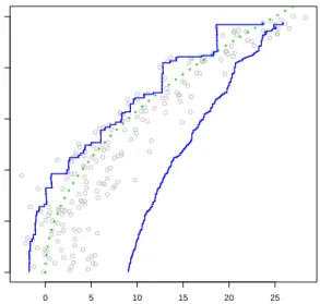
The inconsistency of the m-frontier estimator is illustrated in Figures 1 and 2. The true production frontier in this simulation is given by ϕ(y) =√y and is displayed by the dashed line. We have simulated 200 production inputs from the modelXi=Yi2+Ei, where
Ei ∼Exp(1). The production inputs are then contaminated by an additive noise, so that
the observed inputs are Zi =Xi+εi instead of Xi, whereεi are independently generated
from a zero mean normal variable with standard errorσ = 2.
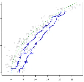
The FDH estimator computed in Figure 1is known to be inconsistent in this situation, because it is constructed under the assumption that all production units are in the produc-tion set Φ with probability one. Figure 2 shows the m-frontier of Cazals et al. (2002) for
m= 1 and 50 respectively (cf. (1.5)). As discussed in Cazals et al. (2002), an appropriate choice ofm is delicate and, as far as we know, there is no automatic procedure to select it from the data. If m is too low, the m-frontier is not a good estimator of the production function. In the theory of Cazals et al. (2002), m is an increasing parameter with respect to the sample size. For large values of y, the estimator is above the true frontier.
For larger values ofm, as shown in Figure2, the estimator is close to the FDH estimator. Because the value ofmincreases withnin theory, the two estimators will be asymptotically close. This illustrates the inconsistency of them-frontier in the case where the noise on the data is not vanishing with increasing sample size.
0 5 10 15 20 25 0 1 2 3 4 5 Z Y
Figure 1: The gray points are the simulated production units and the thick line is the true production frontier. The solid line is the Free Disposal Hull (FDH) estimator of the frontier.
0 5 10 15 20 25 0 1 2 3 4 5 Z Y
Figure 2: Using the same data as in Figure 1, the two solid lines are the m -frontier estimator withm= 1 andm= 50 respectively.
4.2 Robust m-frontier estimation
In order to recover the consistency of them-frontier, we need to plug-in a consistent estima-tor of the conditional survival function in (1.3). The construction of the estimator is easy from the above results if we assume that the additive noise to the inputs is independent from the input X and the output Y. Let y be a point in the output domain where the support of Y is strictly positive. Restricting the data set to (Zi|Yi >y), we can construct
the empirical conditional survival function ˆSZ|Y>y using the usual nonparametric estimator
(1.4). Note that this estimator does not require any regularization parameter such as a bandwidth. In analogy to (3.3), we also define
(ˆδ(n),σˆn) := arg min
δ∈∆(kn,Dn)
σ∈[0,Dn]
γ(Sδ, σ; ˆSZ|Y>y). (4.2)
The final robustm-frontier estimator is then given by ˆ ϕrobm,n(y) = Z ∞ 0 n Sˆδ(n)(u) om du . (4.3)
Note that this integral is easy to compute sinceSˆδ(n)is a step function. The following result
establishes the consistency of this new estimator under a condition on the parameter m.
Proposition4.1. Suppose we observe production units{(Zi, Yi);i= 1, . . . , n}in which the univariate inputs are such that Zi =Xi+εi, where εi models a measurement error that is
independent from Xi and Yi, normally distributed with zero mean and unknown variance
σ2. Consider the robustm-frontier estimator given by equations (4.2) and (4.3) and letmn
be a strictly divergent sequence of positive integers such that
{Sδˆ(n)(ϕ(y))}mn →1 (4.4)
almost surely as n→ ∞. Then ϕˆrobmn,n(y)→ϕ(y) almost surely as n→ ∞.
This result illustrates well the role of the parameter m = mn, which has to tend to
infinity at an appropriate rate as n → ∞ in order to achieve consistency of the robust frontier estimator. Indeed, ifmn is bounded by some M >0, Fatou’s Lemma implies that
almost surely lim n→∞ϕˆ rob mn,n(y)> Z ∞ 0 SX|Y>y(u) M du=ϕ(y) + Z ∞ ϕ(y) SX|Y>y(u) M du.
Except for the trivial case where the true conditional survival function is the indicator func-tion of the interval (−∞, ϕ(y)), the last integral on the right hand side is strictly positive. This shows that the robust estimator asymptotically overestimates the true frontier ϕ(y) ifmn does not diverge to infinity.
On the other hand, ifmn increases too fast in the sense that the condition in (4.4) does
not hold, then ˆϕrob
mn,n(y) may asymptotically underestimate the true frontier ϕ(y) as one can see decomposing the integral from (4.3) into
Z ∞ 0 n Sδˆ(n)(u) omn du= Z ϕ(y) 0 n Sδˆ(n)(u) omn du+ Z ∞ ϕ(y) n Sˆδ(n)(u) omn du.
The second integral on the right hand side tends to 0 almost surely for n → ∞ as we explain in the proof of Proposition 4.1. As for the first one, the integrand converges to a non-negative monotone functionS withS(ϕ(y))<1, and hence the integral may tend to a limit that is smaller than the true frontier ϕ(y). However, this need not be the case, and thus the condition in (4.4) is sufficient but not necessary.
Summarizing the above discussion, the sufficient condition in (4.4) implicitly defines an appropriate rate at which mn may diverge to infinity such that the new robust frontier
estimator is consistent. This rate depends on characteristics of the true conditional survival function, and we do not know at present how to choose it in an adaptive way. Nevertheless, the simulations show that even for finite samples, large choices of mdo not deteriorate the performance of the robust estimator.
The estimator is computed for each possible value ofy. In practice, it is not necessary to estimate the standard deviation of the noise for eachy. We can first estimate the noise level using the marginal data set of inputs only, and use the techniques developed in Section4. We then use this estimated value in (4.2) even as an initial parameter of the optimalgorithm,
or as a fixed, known parameter of the noise standard deviation.
Figure3shows the estimator on the simulated data of Figure1. As for the standardm -frontier, the robustm-frontier with m = 1 is not a satisfactory estimator. The interesting fact about the robust m-frontier is that it does not deteriorate the frontier estimation for large values of m. For the sake of comparison with Figure 2, Figure 3also displays the robustm-frontier estimator withm= 50. This estimator does not cross the true production frontier and does not converge to the FDH estimator.
0 5 10 15 20 25 0 1 2 3 4 5 Z Y
Figure 3: Using the same data as in Figure1, the two solid lines are the robust
5
Conclusion and further research
One original idea in this paper is to consider stochastic frontier estimation when the data generating process has an additive noise on the inputs. The noise is not assumed to vanish asymptotically. In this situation, the m-frontier estimator introduced by Cazals, Florens, and Simar (2002) is still a valuable tool in robust frontier estimation, but it requires to plug-in a consistent estimator of the conditional survival function in order to be consistent itself.
Constructing this consistent estimator is a deconvolution problem. We have solved this problem in this paper. An important feature of our results is that the noise level is not known, and therefore needs to be estimated from a cross section of production units.
Measurement errors are frequently encountered in empirical economic data, and the new robust estimator is designed to be consistent in this setting. The rate of convergence of the estimator is however unknown. This study might be of interest for future research in efficiency analysis.
As it was suggested by a referee, one might also be interested in the case where the measurement error is in the output rather than in the input variable. We would like to end this paper by explaining how the above methods can be transferred to this problem and where the limitations are. In this setting, in contrast to Section 4, the inputsXi are
directly observed, but only a contaminated version
Wi =Yi+ηi, ηi ∼N(0, σ2) (5.1)
of the true output variables Yi is observed, with ηi independent from Xi and Yi. Let us
briefly discuss the case where both the input and the output spaces are one-dimensional, i.e.p=q= 1. As the frontier function ϕ:R+→R+ given in (1.1) is strictly increasing, its
inverse functionϕ−1 :R+ →R+ exists. The efficiency boundary can be described by either
of the functionsϕ and ϕ−1. Estimating ϕ−1 is thus equivalent to estimating ϕitself. The inverse frontier function can be written as
ϕ−1(x) = inf{y∈R+ : FY|X6x(y) = 1},
whereFY|X6xdenotes the conditional distribution function ofY givenX6x. To apply the
robust m-frontier methodology we therefore need to estimate the conditional distribution functionFY|X6x. From the model (5.1), one can easily show that the estimation ofFY|X6x
is again a deconvolution problem, and recalling that FY|X6x = 1−SY|X6x, we can define
(ˆδ(n),σˆn) := arg min
δ∈∆(kn,Dn)
σ∈[0,Dn]
γ(Sδ, σ; ˆSW|X6x) and ˆFn:= 1−Sδˆ(n)
in analogy to Section 4.2. ˆFn is the deconvolving estimator of the conditional distribution
functionFY|X6x. We proceed by defining the robustm-frontier estimator ofϕ−1 as
ˆ ϕ−1m,n(x) :=A− Z A 0 n ˆ Fn(u) om du,
where A > 0 is some constant fixed in advance. Let mn be a strictly divergent sequence
such that {Fˆn(ϕ(x))}mn → 1 almost surely as n → ∞. In analogy to Proposition 4.1, it
can be shown that for such a sequence, ˆϕ−1mn,n(x) is consistent if A > ϕ−1(x). Otherwise, ˆ
ϕ−1
mn,n(x) tends toAalmost surely. This suggests the following adaptive choice of A. First, one computes the estimator with some arbitrary initial value ofA. If the result is close toA, recompute it repeatedly for increasing values ofA until a value smaller thanA is obtained. This estimator is thus robust with respect to noise in the output variable, but note that it is not obvious how to generalize this procedure to a multi-dimensional setting. Moreover, it is not clear how one could cope with a situation with error in both variables. These questions could be subject to further investigation.
A
Proofs
A.1 Proof of Theorem 3.2
In order to show the consistency of the robust frontier estimator, we first need to prove two lemmas.
Lemma A.1. The estimator (Sˆ
δ(n),σˆn) satisfies
γ(Sˆδ(n),σˆn; ˆSnZ)→0 as n→ ∞.
Proof. By the triangle inequality, we have, for any (S′, σ′)∈C×R+,
γ(Sˆδ(n),σˆn; ˆSnZ) = min δ∈∆(kn,Dn) ˜ σ∈[0,Dn] γ(Sδ,σ˜; ˆSnZ) 6 min δ∈∆(kn,Dn) σ∈[0,Dn] γ(Sδ, σ;SX ⋆ φσ) +γ(SX, φσ; ˆSnZ). (A.1)
Let η > 0 and T >0 be such that R∞
T SX(x)dx 6 η/2. For n sufficiently large, we have
σ 6 Dn and there is δ ∈ ∆(kn,Dn) with R0T|(Sδ −SX)(x)|dx 6 η/2, such that
R
R|(Sδ−
SX)(x)|dx 6 η. It follows that the first term on the right hand side of (A.1) is a null sequence, because
γ(Sδ, σ;SX ⋆ φσ)6k(Sδ−SX)⋆ φσkL1 6kSδ−SXkL1kφσkL1 6η.
The second term is also a null sequence by virtue of Glivenko-Cantelli’s and Lebesgue’s
Theorem.
Lemma A.2. The estimator Sˆ
δ(n) defined by (3.3) satisfies
(Pˆδ(n)⋆ φσˆn)
L
−→PZ
Proof. The survival function SZ is continuous everywhere as it can be written as a
convo-lution with some normal density. Therefore, the convergence ˆ
SnZ(x)−−−→n→∞ SZ(x) a.s.
holds for every x∈R. Hence, by Lebesgue’s theorem,
γ(SX, σ; ˆSnZ)−−−→n→∞ 0 a.s.
The triangle inequality, together with LemmaA.1, implies
γ(Sˆδ(n),σˆn;SZ)6γ(Sˆδ(n),σˆn; ˆSnZ) +γ(SX, σ; ˆSnZ) n→∞
−−−→0 a.s.
A continuity argument implies (Sδˆ(n)⋆ φσˆn)(x)
n→∞
−−−→SZ(x) a.s.
for everyx∈R, which is in fact weak convergence and hence concludes the proof. Our proof of consistency also needs the following two lemmas. The first one is quoted from Schwarz and Van Bellegem (2010), the second one is an immediate consequence of Lemma 3.4 from the same article.
LemmaA.3. Let Qn be a sequence of probability distributions and σn a sequence of positive real numbers. Suppose further that (Qn⋆ N(0, σn))n∈N converges weakly to some
probabil-ity distribution. Then, there exist an increasing sequence (nk)k∈N, a probability
distribu-tion Q∞, and a constant σ∞>0 such that
Qnk
L
−→Q∞ and σnk →σ∞
as n→ ∞.
Lemma A.4. A weakly convergent sequence of probability distributions that have all their mass on the positive axis has its limit in P0.
We are now in position the prove the consistency theorem.
Proof of Theorem 3.2. For probability distributions P, P′ and positive real numbers
σ, σ′, define the distance ∆(P, σ;P′, σ′) :=d(P, P′) +|σ−σ′|,whered(·,·) denotes the L´evy distance, which metrizes weak convergence. The theorem is hence equivalent to
∆(Pδˆ(nk),σˆnk;P
X, σ)−−−→n→∞ 0
almost surely. The proof is obtained by contradiction. Suppose that there is some d > 0 and an increasing sequence (nk)k∈N such that
∆(Pδˆnk,ˆσ(nk);PX, σ)> d
By Lemma A.2, we know that the distributions given by (Sˆδ(n)⋆ φˆσn) converge almost surely weakly to PZ. Lemma A.3 implies that there is a distribution P∞, some σ∞ > 0,
and a sub-sequence (n′k)k∈N such that almost surely
Pδˆ(n′
k)
L
−→P∞ and σˆn′
k →σ∞,
which implies the almost sure pointwise convergence of Sδˆ
n′
k
to S∞. Fatou’s lemma then
implies γ(S∞, σ∞;SZ)6lim inf k→∞ γ(Sˆδ(n′k),σˆn ′ k;S Z) = 0 a.s.,
where the last equality holds because of Lemma A.2. Hence, γ(S∞, σ∞;SZ) = 0, and
using continuity again, we conclude thatS∞⋆ φσ∞ =S
X ⋆ φ
σ.Or equivalently, in terms of
distributions, P∞⋆ φσ∞ =P
X ⋆N
σ.As all the distributions Pδˆ(n′
k) have their mass on the positive axis, Lemma A.4 implies that P∞ ∈ P0, and hence that P∞ = PX and σ∞ = σ,
which is in contradiction to the assumption and concludes the proof.
A.2 Proof of Proposition 4.1
We begin the proof by plugging-in the sequencemninto the robust estimator and by splitting
up the integral occurring in (4.3) into
Z ∞ 0 n Sδˆ(n)(u) omn du= Z ϕ(y) 0 n Sδˆ(n)(u) omn du+ Z ∞ ϕ(y) n Sˆδ(n)(u) omn du=:An+Bn
with obvious definitions for An and Bn. We have thatBn→0 almost surely asn tends to
infinity. To see this, let tn:= ϕ(y)∨sup{t∈R : Sδˆ(n)(t) = 1}and decompose Bn further
into Z ∞ ϕ(y){ Sˆδ(n)(u)}mndu= Z tn ϕ(y) 1 du+ Z ∞ tn {Sˆδ(n)(u)}mndu. (A.2)
Firstly,tn→ϕ(y) asn→ ∞because of the consistency ofSδˆ(n). Therefore, the first integral
on the right hand side of (A.2) tends to 0 as n→ ∞. Secondly,Sδˆ(n) is non-increasing and
strictly smaller than 1 on (tn,∞) for every n∈N. As the sequence Sˆδ(n) is further surely
point-wise convergent onR, the other integral of the decomposition in (A.2) also tends to 0.
It remains to show thatAn →ϕ(y) almost surely asn→ ∞. SinceSδˆ(n)is non-increasing
and Sδˆ(n)(0) = 1, we have that sn 6ϕ(y). On the other hand, sn >ϕ(y){Sδˆ(n)(ϕ(y))}mn,
which proves the result by virtue of the assumption.
References
Bigot, J., & Van Bellegem, S. (2009). Log-density deconvolution by wavelet thresholding. Scandinavian
Journal of Statistics,36, 749–763.
Butucea, C., & Matias, C. (2005). Minimax estimation of the noise level and of the deconvolution density in a semiparametric deconvolution model. Bernoulli,11, 309–340.
Butucea, C., Matias, C., & Pouet, C. (2008). Adaptivity in convolution models with partially known noise distribution. Electronic Journal of Statistics,2, 897–915.
Carroll, R., & Hall, P. (1988). Optimal rates of convergence for deconvolving a density. Journal of the American Statistical Association,83, 1184–1186.
Cazals, C., Florens, J.-P., & Simar, L. (2002). Nonparametric frontier estimation: a robust approach.
Journal of Econometrics,106, 1–25.
Daouia, A., Florens, J., & Simar, L. (2009).Regularization in nonparametric frontier estimators(Discussion Paper No. 0922). Universit´e catholique de Louvain, Belgium: Institut de statistique, biostatistique et sciences actuarielles.
Daskovska, A., Simar, L., & Van Bellegem, S. (2010). Forecasting the Malmquist productivity index.Journal of Productivity Analysis,33, 97–107.
De Borger, B., Kerstens, K., Moesen, W., & Vanneste, J. (1994). A non-parametric free disposal hull (FDH) approach to technical efficiency: an illustration of radial and graph efficiency measures and some sensitivity results. Swiss Journal of Economics and Statistics,130, 647–667.
Delaigle, A., Hall, P., & Meister, A. (2008). On deconvolution with repeated measurements. The Annals of Statistics,36, 665–685.
Deprins, D., Simar, L., & Tulkens, H. (1984). Measuring labor inefficiency in post offices. In M. Marchand, P. Pestieau, & H. Tulkens (Eds.),The performance of public enterprises: Concepts and measurements
(pp. 243–267). Amsterdam: North-Holland.
Fan, J. (1991). On the optimal rate of convergence for nonparametric deconvolution problems. The Annals
of Statistics,19, 1257–1272.
F¨are, R., Grosskopf, S., & Knox Lovell, C. (1985). The measurements of efficiency of production (Vol. 6). New York: Springer.
Hall, P., & Simar, L. (2002). Estimating a changepoint, boundary, or frontier in the presence of observation error. Journal of the American Statistical Association,97, 523-534.
Johannes, J., & Schwarz, M. (2009). Adaptive circular deconvolution by model selection under unknown
error distribution (Discussion Paper No. 0931). Universit´e catholique de Louvain, Belgium: Institut de statistique, biostatistique et sciences actuarielles.
Johannes, J., Van Bellegem, S., & Vanhems, A. (2010). Convergence rates for ill-posed inverse problems
with an unknown operator. Econometric Theory. (forthcoming)
Johnstone, I., Kerkyacharian, G., Picard, D., & Raimondo, M. (2004). Wavelet deconvolution in a periodic setting. Journal of the Royal Statistical Society Series B,66, 547–573.
Kneip, A., Park, B., & Simar, L. (1998). A note on the convergence of nonparametric DEA estimators for production efficiency scores. Econometric Theory,14, 783–793.
Leleu, H. (2006). A linear programming framework for free disposal hull technologies and cost functions:
Primal and dual models. European Journal of Operational Research,168, 340–344.
Li, T., & Vuong, Q. (1998). Nonparametric estimation of the measurement error model using multiple indicators. Journal of Multivariate Analysis,65, 139–165.
Meister, A. (2006). Density estimation with normal measurement error with unknown variance. Statistica
Sinica,16, 195–211.
Meister, A. (2007). Deconvolving compactly supported densities. Mathematical Methods in Statistics,16,
195–211.
Meister, A., Stadtm¨uller, U., & Wagner, C. (2010). Density deconvolution in a two-level heteroscedastic model with unknown error density.Electronic Journal of Statistics,4, 36–57.
Neumann, M. H. (2007). Deconvolution from panel data with unknown error distribution. Journal of
Multivariate Analysis,98, 1955–1968.
Park, B. U., Sickles, R. C., & Simar, L. (2003). Semiparametric efficient estimation of AR(1) panel data models. Journal of Econometrics,117, 279-311.
Park, B. U., Simar, L., & Weiner, C. (2000). The FDH estimator for productivity efficiency scores: asymp-totic properties. Econometric Theory,16, 855–877.
Pensky, M., & Vidakovic, B. (1999). Adaptive wavelet estimator for nonparametric density deconvolution.
The Annals of Statistics,27, 2033–2053.
Schwarz, M., & Van Bellegem, S. (2010). Consistent density deconvolution under partially known error distribution. Statistics and Probability Letters,80, 236–241.
Seiford, L., & Thrall, R. (1990). Recent developments in DEA: The mathematical programming approach to frontier analysis. Journal of Econometrics,46, 7–38.
Shephard, R. W. (1970). Theory of cost and production functions. Princeton, NJ: Princeton University
Press.
Simar, L. (2007). How to improve the performances of DEA/FDH estimators in the presence of noise?
![Table 2: The inputs simulated in this experiment are a mixture U [1, 2] + Exp(1).](https://thumb-us.123doks.com/thumbv2/123dok_us/887197.2613828/10.892.359.558.198.414/table-inputs-simulated-experiment-mixture-u-exp.webp)