https://doi.org/10.1007/s00500-018-3561-7
M E T H O D O L O G I E S A N D A P P L I C A T I O N
An Evolutionary Algorithm and operators for the Airport Baggage
Sorting Station Problem
Amadeo Ascó1
© The Author(s) 2018 Abstract
Taking into consideration the constraints and objectives to appropriately assigning the available airport resources throughout the period of time an airport provides its services can greatly affect the quality of service which airlines and airports provide to their customers. The appropriate assignments can help airlines and airports to keep to published schedules, by minimising changes in these schedules, reducing delays and considering customers preferences when assigning the resources. Given the expected increases in civil air traffic, and the variety of resources, the complexities of resource scheduling and assignment continue to increase. For this reason, as well as the dynamic nature of the problems, scheduling and assignment are becoming increasingly more difficult. An Evolutionary Algorithm is presented together with some different operators, which are used to find good solutions to the Airport Baggage Sorting Station Assignment Problem for when there are not sufficient resources up to when the number of resources is sufficient to fulfil the demand on these resources. The contributions of these different operators are studied and compared to other approaches, giving insights into how the appropriate choice may depend upon the specifics of the problem at the time.
Keywords Airport Baggage Sorting Station Problem·Scheduling·Heuristics·Evolutionary Algorithms
1 Overview
Many airport resources (for example, stands, gates, tugs, stor-age points, fuel trucks and baggstor-age stations) are of limited availability and are expensive or time-consuming to increase in quantity. Given this, airports need to use their resources as efficiently as possible, since any delays due to lack of available resources can have a direct impact upon the pub-lished schedules, the provision of services to customers and the workforce. Moreover, the characteristics of each problem are represented by constraints and the desired solutions by objectives, which naturally conflict with each other.
The problem can be represented by some constraints which must be strictly complied with (known as hard con-straints) and other constraints where compliance is desirable (called soft constraints or objectives). In order to solve a prob-lem, it is necessary to find solutions which comply with both
Communicated by V. Loia.
B
Amadeo Ascó1 University of Nottingham, Sandbach, Moston, UK
the hard constraints and most or all of the soft constraints. An indication of the compliance with the soft constraints is provided by an evaluation function, sometimes referred to as the fitness function, the results of which give an indication as to the quality or fitness of the solutions.
Many approaches have been used to solve optimisa-tion problems, like the Airport Baggage Sorting Staoptimisa-tion Assignment Problem (ABSSAP), two of which are Genetic Algorithms (GAs) and Tabu Search (TS). GAs are one of the methodologies belonging to the population-based model of Evolutionary Algorithms (EAs), based on the Darwin and Wallace (1858) theory of natural selection and Mendelian genetics (Mendel1865), which are recognised as the foun-dation of evolutionary biology. GAs have been used to solve a wide range of airport problems, such as the Airport Gate Assignment Problem (AGAP) in Lim et al. (2005), the scheduling of arriving aircraft in Cheng et al. (1999), Xiang-wei et al. (2010) and Hansen (2004), the scheduling of depart-ing aircraft in Bolender (2000) and Caprì and Ignaccolo (2004), the aircraft taxiing in Gotteland and Durand (2003) and the ABSSAP in Ascó (2016) and Ascó et al. (2010,2012,
2013). TS is a Metaheuristic algorithm which employs a local search, which in turn uses a solution to generate a
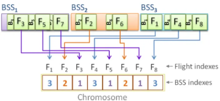
neighbour-Fig. 1 An example of encoding for a three BSSs and eight flights hood of solutions. The solutions from the neighbourhood are checked in the hope of finding an improved solution. A local search may get stuck within areas of the search space where the neighbourhood is equally fit, so memory structures which describe the neighbourhood visited are incorporated to avoid using again solutions and regions previously visited, Glover (1989,1990) and Burke and Kendall (2005). An implementa-tion of both a GA and TS is used later in this paper, where the neighbourhood (also called local walk) is generated by using the mutation operators described in Sect.6, which constitute the list of candidate solutions. In the TS, the fittest non-tabu solution in the candidate list is adopted as the new current solution and is also added to the tabu list. Once the tabu list is full, one solution is removed from the tabu list to leave space for the new tabu solution.
Various different ABSSAP objectives have to be consid-ered, such as maximising assignments, ensuring full service time and allocating preferential positions. Some of these objectives are in obvious conflict (reducing service times in order to service an additional flight, for example), thus preventing simultaneous optimisation of each objective.
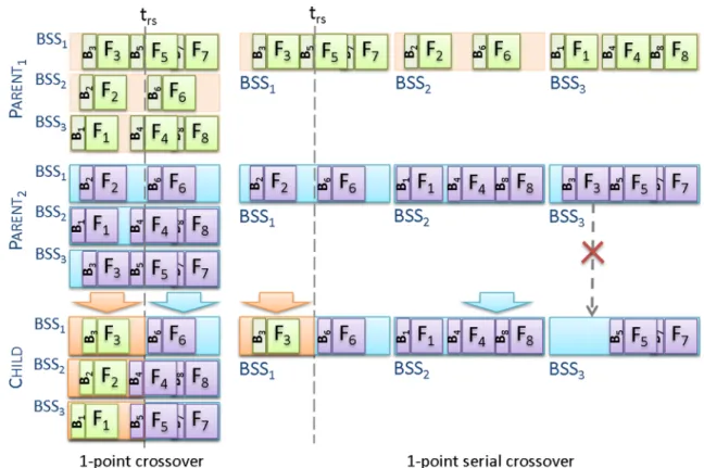
An encoding of the parameter set for the ABSSAP for the Canonical Genetic Algorithm (CGA) was implemented using the Evolutionary Computation Java library (ECJ), where a chromosome is composed of the indexes of the baggage sort-ing station (BSS) assigned to each flight, the flights besort-ing ordered by their base service starting time, as shown in Fig.1. The initial studies showed that good initial solutions greatly improve the speed, convergence and quality of the final solutions to the limited time ranges under considera-tion, as shown in Sect.8.
The following sections begin by a description of the prob-lem, followed by a description of the proposed EA with its operators and selectors, followed by a study of the problem, using a fitness function as a single compound objective which represents realistic priorities.
2 The Airport Baggage Sorting Station
Assignment Problem
The checked-in baggage at a passenger airport first enters the baggage system where it is processed and delivered to
the ground side, and an overview of the process is provided in Fig.2. The baggage is then transported by conveyor belts to the baggage system’s security hall where it is individually scanned. Most baggage will continue straight on, but if at the scanning stage suspicions were aroused concerning the bag-gage, then it is diverted to the security checking area where it will be further checked by one of the security personnel and, if clear, will rejoin the normal journey with the rest of the baggage. In the area of conveyor systems, Johnstone et al. (2015) investigate the design and control of merging bot-tlenecks of conveyor-based baggage handling systems, and Kim et al. (2017) looks at determining an appropriate work-load balance for a Baggage Handling System (BHS). The baggage will then continue (on conveyor belts) to the bag-gage hall and be transported to the bagbag-gage sorting station assigned to it. Once the baggage reaches the BSS, it accu-mulates ready for the workforce to sort and place on trolleys or into special containers, which go directly into the aircraft, ready for transportation by cart and placed next to the aircraft on the air side where the baggage is loaded into the aircraft hold by the ground workforce, ready to travel to its destina-tion. Containers are used to transport the baggage on wide fuselage aircraft, for long distance flights, which are directly placed into the hold of the aircraft. The proposed EA here assigns these BSSs to the aircraft (flights) under the described constraints and objectives presented in Sect.3. Trolleys are used in the narrow fuselage aircraft, and the baggage is indi-vidually loaded into the hold of the aircraft by the handling workforce, who use conveyor belts to lift the baggage from the trolleys to the level of the aircraft’s hold. Johnstone et al. (2010) looked at the routing of the baggage within the bag-gage system with the aim of providing additional insight into how agents can learn to route in a baggage handling system, and experiments show that the learning method performs bet-ter than the search method.
On reaching the destination airport, the process is reversed, so that the ground workforce removes the baggage from the cargo area of the aircraft and places it directly on baggage carts (open trolleys, onto which baggage is separately loaded and protected with a canvas cover) or loads in baggage con-tainers onto dollies (trailers, on which baggage concon-tainers are loaded) ready for transportation by cart to the baggage sorting stations assigned. Here the handling force transfers it from the trolleys or containers onto the baggage sorting sta-tions for transportation to the ground side of the arrival hall. The baggage then enters the baggage system which delivers the baggage to the carousel to which the flight is assigned, in readiness for collection by the corresponding owner, and will then leave the airport. In the case of transfer passengers, their baggage is delivered to the baggage sorting station assigned to their next flight. The sorting station used by a flight arrival is normally directly linked to the carousel assigned to the passenger flight for the given destination, and only the
trans-Fig. 2 Simplified overview of baggage system
fer baggage re-enters the baggage system for delivery to the sorting station assigned to its next departure, as shown in the ‘Arrival hall’ in Fig.2. The transfer baggage does not usu-ally need to be directed through the security hall, given that it should already have been checked at the original airport.
Where airports have several terminals, it would be unreal-istic to assume that baggage from a flight at a terminal stand is serviced by a baggage sorting station in another terminal (e.g. passengers usually go through security and board flights from the terminal at which they checked their baggage in). This may not be the case for transfers where passengers and their baggage arrive at an airport terminal and perhaps leave the airport by another flight departing from a different termi-nal.
The ABSSAP involves the assignment of BSSs to flights already scheduled. These previously scheduled flights have already been assigned to stands, which are the areas allocated for parking aircraft, and the stand is required from the time of arrival to the time of departure, whereas gates are the areas in a terminal where passengers access the aircraft. In the AGAP, when practitioners refer to the assignment of flights to gates
they mean the assignment of the stands associated with these gates, normally located at a pier next to the gate.
3 A model of the problem under study
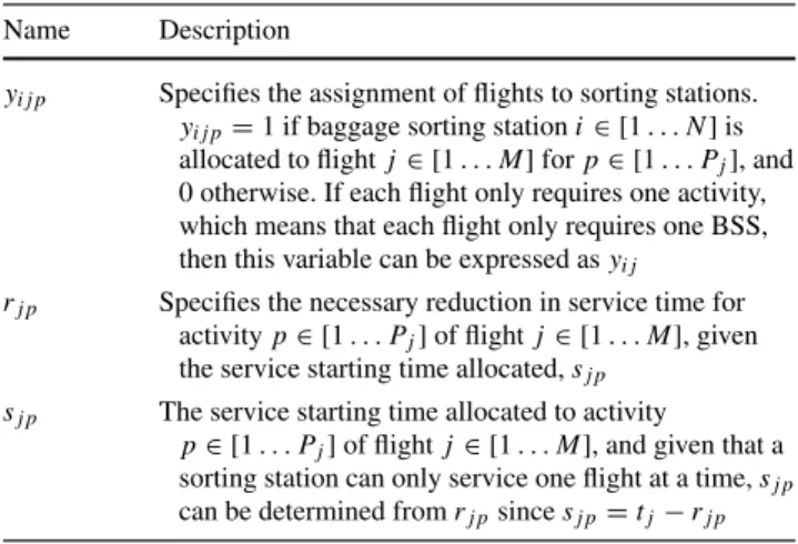
The problem is composed ofN BSSs, andM flights, where flightjrequiresPjactivities to be completed, each of which must be serviced by a different BSS. The objective here is to find appropriate values for the yi j p Boolean variables, which take a value of 1 if activitypof flightjis assigned to baggage sorting stationi, or zero otherwise, with a service starting timesj pand reduction in service timerj pallocated to activitypof flightj. The target service time represents the time in which a BSS is expected to be assigned to a flight. The reduction in service time has a detrimental effect on the robustness of assignments against real-life delays. Therefore, the amount of reduction in the target service time for the assignment of an activitypfor flight jis represented byrj p, which is calculated in seconds (as an integer). The described variables are shown in Table1. A study of different
robust-Table 1 Decision and input variables for this ABSSAP model Name Description
yi j p Specifies the assignment of flights to sorting stations. yi j p=1 if baggage sorting stationi∈ [1. . .N]is allocated to flightj∈ [1. . .M]forp∈ [1. . .Pj], and 0 otherwise. If each flight only requires one activity, which means that each flight only requires one BSS, then this variable can be expressed asyi j
rj p Specifies the necessary reduction in service time for activityp∈ [1. . .Pj]of flightj∈ [1. . .M], given the service starting time allocated,sj p
sj p The service starting time allocated to activity
p∈ [1. . .Pj]of flightj∈ [1. . .M], and given that a sorting station can only service one flight at a time,sj p can be determined fromrj psincesj p=tj−rj p
ness approaches for the ABSSAP has been presented in Ascó (2016).
There are some constraints to be complied with within the ABSSAP:
Assignment Limitseach flight must be assigned to at most
Pj BSSs, as expressed by Inequality1. N
i=1
yi j p ≤Pj ∀j ∈ [1. . .M]and∀p∈ [1. . .Pj] (1)
Complete Assignmentwhen Pj > 1, the activities
cor-responding to the same flight must either all be assigned or none should be assigned, as expressed by Formula2.
N i=1 yi j p= N i=1 yi j(p+1)∀j∈ [1. . .M]and∀p∈ [1. . .Pj−1] (2)
Reduction in ServiceBSSs can only be used by one flight at
a time, so it may be necessary to reduce the flight service time (usually by reducing the buffer times between flights) in order to assign flights to the same sorting station. The principal objective is usually to maximise the number of assignment of BSSs to flights.
For any pair of different flights where service times overlap, if the overlap in service times is greater than the maximum reduction allowed (Blq for activityq of flightl), then both flight activities cannot be assigned to the same BSS. Thus, Inequality3applies to any such pair of flights, jandl
(j =l), wheretlq<ej ≤el and(ej−tlq) > Blq.
yi j p+yilq≤1 (3)
They may otherwise be assigned to the same BSS as long as the service duration of flightl is sufficiently reduced to remove the overlap. Inequality4applies to any such pair of
flights, jandl(j =l), and their activities pandq, respec-tively, where tlq < ej ≤ el and(ej −tlq) ≤ Blq. One objective is to minimise these service time reductions.
rlq≥(yi j p+yilq−1)∗(ej−tlq) (4)
Limit of Service Reductionthe reduction in service
dura-tion may not exceed a limit, as expressed by Inequality5.
0≤rj p ≤Bj p ∀j ∈ [1. . .M]and∀p∈ [1. . .Pj] (5) A number of objectives concerning this problem need con-sideration, and there is a trade-off to be made amongst them. The various objectives considered in this section are:
1.Maximise Assignment of Baggage Sorting Stationsthe
first and most important objective is to maximise the number of flights assigned to BSSs, as expressed by Formula6.
f1=max N i=1 M j=1 ⎛ ⎝ Pj p=1yi j p Pj ⎞ ⎠ (6)
2.Robustnessdelays on the day of operation may render
some assignments infeasible which need to be reassigned. It is therefore desirable to account for potential delays on the day of operation when generating the flight assignments to BSSs at the planning stage, such that the final flight assign-ments differ little or not at all from the original assignassign-ments on the day of operation. The degree to which this is achieved is an indication of the solution robustness, so a solution which requires less in reassignments is said to be more robust than those solutions requiring more reassignments. Robustness is the ability of assignments to resist changes consequence of perturbations by reducing or removing the need to reassign current assignments. One of these approaches is to Minimise Reduction in Service, as expressed by Eq. 7. A study of robustness approaches for the Airport Baggage Sorting Sta-tion Problem (ABSSP) is presented in Ascó (2016) and Ascó (2013). f2=min M j=1 Pj p=1 rj p (7)
3. Minimise Distance the distance between the BSSs
which are assigned to the flights and the flights to which they are assigned should be as short as possible. This objective aims to minimise the inconvenience, work and time involved in getting baggage to the aircraft and could reflect preferences rather than distances. One way to handle this objective would be by expressing it as in Formula8whereiN=1
yi j p∗di j represents the distance between flightjand its allocated BSS
Fig. 3 Representation of the different times for activityp. f3=min M j=1 Pj p=1 Cj p∗ N i=1 yi j p∗di j (8)
Other objectives may be considered, such as Consecutive Assignments, Fair Workload, Preferred Piers and Flights to the Same Destination, between others. Some of these other objectives were looked at in Ascó et al. (2013) and Ascó et al. (2011).
A fitness function composed of the weighted sum of the three first objectives presented above was used to guide the search within the algorithm, expressed by Eq.9whereWi is the weight for objectiveiand fi is the corresponding objec-tive function. f = 3 i=1 Wi ∗ fi (9)
Flights which cannot be assigned to any BSS are assigned to the dummy BSS, an approach widely used in the AGAP, as shown in Tang et al. (2009) , Drexla and Nikulina (2008) and Yan and Huo (2001).
The constants of the model are shown in Table2, and the relationship between the timing values is illustrated in Fig.3. A full description of the ABSSAP can be seen in Ascó (2013). The following two points were defined from the flight density for the day under study and will be observed to be useful later when interpreting the results for the ABSSAP.
The Lower Maximum Assignment Point (LMAP) is the
number of resources required to service a certain number of activities when the service starting time (sj p) coincides with the target starting service time (tj p), as shown in Fig.4.
TheUpper Maximum Assignment Point (UMAP) is the
number of resources required to service those activities when the service starting time (sj p) coincides with the base starting service time (τj), as shown in Fig.5.
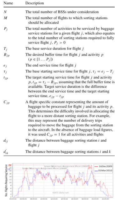
Table 2 Constants and input values for this ABSSAP model Name Description
N The total number of BSSs under consideration M The total number of flights to which sorting stations
should be allocated
Pj The total number of activities to be serviced by baggage service stations for a given flightj, which also equates to the total number of sorting stations required to fully service flight j,Pj>0
Tj The base service duration for flight j
Bj p The desired buffer time for flight jand activityp (p∈ [1. . .Pj])
ej The end service time for flight j
τj The base starting service time for flightj,τj=ej−Tj tj p The target starting service time for flight jand activity
p,tj p=τj−Bj p, assuming that the full buffer time is available. Target service duration is the difference between the end service time and the target starting service time,ej p−tj p
Cj p A flight specific constant representing the amount of baggage to be processed for flightjand its activityp. This determines the difficulty involved in allocating the flight to a more distant sorting station. For example, this may represent the number of delivery trips required to move the baggage from the sorting station to the aircraft. In the absence of baggage load figures, it was usedCj p=1 for all activities and flights di j The distance between baggage sorting stationiand
flight j
di k The distance between baggage sorting stationsiandk
Fig. 4 LMAP for both 16/13/2009 and 01/03/2010
4 Steady-State Evolutionary Algorithm
A Steady-State GA maintains the majority of the population between iterations, only replacing a few individuals at each iteration, a term initially introduced in Syswerda (1989). In the Steady-State Evolutionary Algorithm (SSEA) presented here, Algorithm1, the next population is obtained by apply-ing the population selection operator, some of which are introduced in Sect. 5-1, to the current population. One of the operators is applied to the individuals selected from the population by the member selector (Sect.5-2), this last step being called an iteration and being repeatedtimes, known as a generation. The newly obtained individuals are added to the population so constituting the current population. This is repeated until the termination condition is reached. In contrast to the CGA, parents and offspring typically coexist such that the parents are also considered for the next genera-tion, which theoretically increases the algorithm’s ability to retain information for exploitation in subsequent generations. This creates additional selective pressure towards informa-tion already contained in the populainforma-tion. However, keeping the parents does not provide the search with new informa-tion since it does not sample new genotypes. The approach may incorporate an ageing strategy to ensure that the parents eventually leave the population, thus increasing the chance of offspring contributing to building the next population. Schwefel and Rudolph (1995) incorporated an age by defin-ing a maximum duration of life, so any individual survivdefin-ing longer than this will be worse than any other which has not reached such limit or has less fitness.The SSEA is an instance of the Evolutionary Strategies (ESs) which can be described as (μ+λ)-ES, 1≤λ, where
λmay be greater thanμ. In the case of the SSEA considered here where the operators used provide only one offspring, when applied,λ=. A Steady-State GA considering parents in the next generation was presented in Whitley (1989) and Whitley and Kauth (1988), which differs from a CGA in that it uses a serial recombination wherein an offspring replaces the lowest ranking individual in the population rather than the parent, whereas the SSEA may use some or all of the parents in the next generation since the next population in a generation is built by applying the replacement strategy to the current population, which in turn is composed of both the off-spring and the parents, so the chance of a parent taking part in the next generation is determined by the replacement strategy used. The SSEA makes use of two selectors,Spwhich selects the population which is to take part in the next generation and
Smwhich selects the member(s) from within an iteration to which the chosen operator is applied. Likewise, Sokolov and Whitley (2005) follows similar steps when generating their GA; the main difference to the SSEA is the use of, two selection processes and the operators being any combination of operators. The initial population may also be composed
Algorithm 1:SSEA Input: Initial populationP0
Input: Number of iterations in a generation∈Z+, >0
Input: Operators;Oj∀j∈ [1. . .R] Input: Replacement strategies,Sp Input: Parent(s) selector,Sm
1 begin
// Initialisation
2 P←P0;// set inital population // Execution of generations 3 repeat
4 P←Sp(P);// apply replacement strategy
to get the new population
5 Pt← ∅;// empty population of children
6 i=1;// initialise the iterations // Execution of iterations 7 repeat
8 Select an operator,Ok;
9 Q←Sm(P,Ok);// select parents
10 Q←Ok(Q);// generate children
solutions by applying operator 11 Pt←Pt∪Q;// add children solutions
to the population of children 12 i=i+1;// increment iteration 13 untili≤or Termination Condition; 14 P←P∪Pt;// merge parents with
children solutions 15 untilTermination Condition; 16 returnP;
17end
of fewer solutions than the preferred population size. This size should eventually be reached as the new solutions gen-erated are merged with the parent solutions, and then, the replacement strategy is applied.
For = μ(the population size), the SSEA algorithm is closer to a CGA, but still differs from the CGA in that:
1. The new population to which the replacement strategy is applied is of sizeμ+λ, whereas for the CGA it isλ. Thus, not only do parents and offspring coexist in the new population, but also those previous solutions which may not have been selected for the generation of offspring in the current generation.
2. A generation is composed ofiterations in which par-ents are selected and operators applied to generate the offspring, which together with the previous population will compose the current population.does not need to be fixed, and it can be changed as the search progresses, thus providing an additional mechanism to control the sampling.
3. Whereas in the CGA reproduction produces two off-spring, in the SSEA the reproduction may produce either one or many offspring.
4. In the CGA up to two operators may be applied, namely crossover and mutation. The SSEA does not put any restriction on the operator, so operators may be applied one per iteration or a set of operators in an iteration, as described in the following sections. An operator may be defined which sequentially applies a set of sub-operators to the offspring of the previous operator, based on some criterion, such as the probability of a sub-operator being selected. An example of this is where two operators are used one with a probability of 1, so it is always used, and a second operator a probability of 0.1 being used. The first offspring is always obtained by applying the first operator to the parents in the population, given its prob-ability of 1. This offspring may be further modified by the second operator in order to obtain the final offspring; otherwise, where the second operator is not applied, the first offspring becomes the final one. If both probabili-ties are lower than 1, there is a chance of the parent also becoming the final offspring.
5. Each operator has a probability associated with it which represents the chance of being selected, where the overall probability of selecting any of the operators totals 1. In this SSEA, any of the operators may be selected at each iteration based on their probabilities.
5 Selectors
The selector methods are responsible for selecting solutions within a population of solutions. Two types of selector are used throughout this paper which are:
1. Replacement Strategies(Sp) The replacement strategies
generate the new population from the parents and off-spring which is used in the following generation. The replacement strategies are used in both CGA and SSEA. They distribute the chance of individuals taking part in the next generation. Normally, the fitter the solution, the more chance it has of being selected for participation in the following generation. A comprehensive analysis of selection schemes used in EAs can be found in Blickle and Thiele (1996).
2. Parent Selectors (Sm) The member selectors distribute
the chance of a given solution within the population tak-ing part in generattak-ing new offsprtak-ing within a generation. Normally, the fitter the solution, the more chance there is of being selected to produce new offspring.
An increase in diversity certainly corresponds to broaden-ing exploration of the search space, and findbroaden-ing an adjustable balance between exploration and exploitation is the key, Levinthal and March (1993) and March (1991). Exploration and exploitation should not be constrained to specific parts
of the process, such as only in the early stages of the search, but also be taken into account throughout all the evolutionary processes based on the characteristics at each stage.
The selection of solutions for participation in a popula-tion is one of the mechanisms for managing diversity, which together with the operators helps to improve the direction of the search within the domain of solutions into the regions containing solutions with a higher potential.
Some of the terms used are defined below which are based in Baker (1987) and Blickle and Thiele (1996).
– Selective pressureis the probability of selecting the best
individual compared to the average probability of selec-tion of all the individuals.
– Biasis the absolute difference between an individual’s normalised fitness and its expected probability of repro-duction.
– Spreadis the range of possible values for the number of
offspring of an individual.
There follows an overview of the new approaches pro-posed.
5.1 Stochastic Universal Modified Sampling
The Stochastic Universal Sampling (SUS) may not be appro-priate when the order of magnitude of the fitness under study is greater than the difference in the fitness values amongst individuals; such are the cases studied in this paper. So Stochastic Universal Modified Sampling (SUMS) is defined in such a way as to provide a greater selection pressure, as shown in Algorithm2. SUMS provides more selection pres-sure than SUS and some bias. A characteristic of the SUMS is that offsetting of all of the fitness by a constant does not affect those sections of the roulette wheel occupied by each solution as this is not the case for the SUS.
In both versions, a single spin of the roulette wheel is made which provides both a starting point and the first individual. The following selections are made by advancing the point in equal step sizes and selecting the individual occupying the section upon which the point fell: the process is repeated until all the required individuals have been selected. Some individuals may not be selected where their occupied section is sufficiently small, depending on the starting point.
Both versions of sampling ensure that the observed selec-tion frequencies of each individual are in line with the expected frequencies. So if there is an individual occupying 6.5% of the wheel and it is necessary to select 100 individ-uals, it is expected, on average, that that individual will be selected between six and seven times. Whereas both SUS and SUMS guarantees this, roulette wheel selection does not make such a guarantee.
Algorithm 2:Stochastic Universal Modified Sampling Input: PopulationPof sizeλ
Input: Desired population size ofμ, 0< μ < λ
begin
// Calculate the two lowest fitness
Fmi n= ∞; Fmi n−1= ∞; fori=1→λdo ifFmi n> fithen Fmi n−1=Fmi n; Fmi n= fi; end else ifFmi n> fithen Fmi n−1= fi; end end F=Fmi n−(Fmi n−1−Fmi n);
// Assign a section to each solution
p0=0; fori=1→λdo pi= i j=1(fj−F) λ j=1(fj−F); end // Initialise
P← ∅;// empty next population
r0=r nd
0,μ1
;// identify first point
i=1;// set to first solution in P // Select members from the population
based on their roulette wheel section
forj=1→μdo r=(j−1μ)+r0; fori→λdo
ifpi>rthen
P←i;// add selected solution to next population break; end end end returnP; end
5.2 Index selector (ISxy)
This new selector makes sure that no more than a fixed max-imum number of fitness duplicates are selected for the next population. This selector requires an integer which corre-sponds to the maximum number of solutions with the same fitness to keep (x, number of solutions) and a base selector (y, the base selector), one of the selectors presented above, e.g. the Index Selector with the Elitist Selector and a group size of 1 would be represented asI S1E S.
The Index Selector is only useful as a replacement strategy, given that as a parent selector it merely selects a very reduced number of solutions.
5.3 Range index selector (RISxyz)
Empirical results show that when the previous selector ISxy was applied to the ABSSAP, different groups with small dif-ferences were generated, which also represented a reduction in diversity, and which diversity may be increased further by changing the ISxy from a unique fitness in each group to a range of fitness per group. This requires a knowledge of group size (x, the maximum number of solutions to be kept within a range), a base selector (y, the base selector) and an indication of the fitness range (z), e.g. the Range Index Selec-tor with Elitist SelecSelec-tor (y=ES), a group size of 1 (x=1) and fitness range of 50 (z=50) which may be represented as
R I S1E S50. For R I S1E S50 and a maximisation problem,
if the group having a fitness range from 1000 to 1050 already contains a solution with a fitness of 1000, and a new solution is to be added to the population with a fitness of 1010, then the solution of a 1000 is removed and the new solution is introduced into the group in its place, given thatx=1. The selection within a group uses a greedy approach.
Many of the selection approaches presented are not suit-able where only one individual (solution) is required, as is the case for the Index Selection (ISxy) and Range Index Selec-tor (RISxyz), given that in those cases they are equivalent to the underlying selection approach, e.g. the Index Selection with Elitist Selection (ISxES) is the same as the Elitist Selec-tion (ES). Such is the case for the mutaSelec-tion operators (Sect.6) where the Parent Selectors have to select only one parent solu-tion. Similarly, some of the classic selection methods such as SUS, Roulette Wheel Member Selection (RWMS) and Tour-nament Member Selection (TMS) are equivalent when just one parent solution has to be selected.
6 Operators
Two main groups of operators are reviewed in the following sections: Mutation and Crossover. Both of these are described below.
6.1 Mutation
The operators introduced here are local search (guided muta-tion) operators which generate feasible solutions.
All flights which have not been assigned to a sorting station are assigned to the ‘dummy’ sorting station. Some operators can switch flights between the real and dummy sorting sta-tions.
When a sorting station is to be selected, the roulette wheel selection method is used whereby every sorting station has the same probability of being selected.
When a time has to be determined (for instance for the start or end of a time range), a uniform random variable is used,
so that any time within the time range of the flights under consideration has an equal probability of being chosen. 6.1.1 Dummy Single Exchange Mutation Operator (DSEMO) The DSEMO is equivalent to the ‘Apron Exchange Move’ used by Ding et al. (2004,2005). A solution is selected from the population by the member selector (Sm); then, a new
solution is built by moving a flight from the ‘dummy’ sorting station in this solution to a randomly selected sorting station, thus potentially moving another flight back onto the ‘dummy’ sorting station where it can no longer be fitted in.
This operator may increase the number of assignments where the operation does not move a flight back onto the ‘dummy’ sorting station.
It is necessary that some flights be unassigned in the parent solution. So when full assignment has been attained for the given number of BSSs, this operator clearly will not provide a new solution.
6.1.2 Dummy Single Move Mutation Operator (DSMMO) In the DSMMO, a random unallocated flight and initial target sorting station are chosen, and an attempt is made to assign the flight to the selected sorting station. If the assignment cannot be achieved, then the next sorting station is selected and the process is repeated until the flight is assigned, or no more sorting stations are available, in which case the flight is returned to the ‘dummy’ sorting station. When maximum assignments have been attained for the given number of sort-ing stations, this operator obviously will not provide a new solution.
6.1.3 Multi-Exchange Mutation Operators
A set of sorting stations is randomly selected from these oper-ators within a random time period,tr stotr e. All assignments where the base service durations are entirely within the time period are then moved to the next sorting station in the set, as shown in Fig.6, provided they fit. This operation is repeated from one sorting station in the set to the next, until they have all been covered. Flights which cannot be moved are added to the set of flights which will be considered for assignment at the end, potentially reducing the number of flights which would otherwise not be assigned. These operators generalise the ‘Interval Exchange Move’ which was presented by Ding et al. (2005), and cannot increase the number of assignments.
Three variants have been developed:
1. Multi-Exchange between a Fixed Number of Resources (MEFNRn): The number of sorting stations between which flights are exchanged is fixed at n, where 2 ≤
n≤ N.
Fig. 6 Example of multi-exchange between three BSSs
2. Multi-Exchange between a Random Number of Resour-ces (MERNRn): The number of sorting stations between which flights are exchanged is randomly chosen each time, between 2 andn, where 2<n≤ N.
3. Multi-Exchange between a Range Random Number of Resources (MERRNRxy): The number of sorting stations between which flights are exchanged is randomly chosen each time, betweenxandy, where 2≤x<y≤N. 6.1.4 Multi-Exchange By Pier Mutation Operators
These operators are a specialised case of the Multi-Exchange Mutation Operators, where the sorting station selection ele-ment ensures that no two consecutive sorting stations in the set are on the same pier. The idea is to improve the dis-tance objective by encouraging the movement of assignments between piers.
Once again, this operator cannot increase the number of assignments. As for the Multi-Exchange Mutation Operators, three variants have been created:
1. Multi-Exchange By Pier between a Fixed Number of Resources (MEBPFNRn): The number of sorting sta-tions to exchange flights between is fixed atn, where 2≤n≤ N.
2. Multi-Exchange By Pier between a Random Number of Resources (MEBPRNRn): The number of sorting stations between which the flights are exchanged is ran-domly chosen each time, between 2 andn, where 2 <
n≤N.
3. Multi-Exchange By Pier between a Range Random Number of Resources (MEBPRRNRxy): The number of sorting stations between which the flights are exchanged is randomly chosen each time, betweenxandy, where 2≤x<y≤N.
6.1.5 Range Multi-Exchange Mutation Operators
These are the same as the Multi-Exchange Mutation Oper-ators; however, they add an additional feasibility recovery step when flights cannot be moved. Flights which cannot be
Fig. 7 Example of range multi-exchange between three BSSs
moved are added to the set of flights which will be consid-ered for assignment to the next sorting station, potentially reducing the number of flights which would otherwise not be assigned at the end. Finally, flights which have still not been moved are again considered for assignment to the other sorting stations in the set, except the last one, once again potentially reducing the number of flights which otherwise would not be assigned, in the same way as the Multi-Exchange Mutation Operators, as shown in Fig.7.
Once again, this operator cannot increase the number of assignments. Three variants have been developed:
1. Range Multi-Exchange between Fixed Number of Res-ources (RMEFNRn): The number of sorting stations between which to exchange flights is fixed atn, where 2≤n≤ N.
2. Range Multi-Exchange between Random Number of Resources (RMERNRn): The number of sorting stations between which to exchange flights is randomly chosen each time, between 2 andn, where 2<n≤N.
3. Range Multi-Exchange between Range Random Num-ber of Resources (RMERRNRxy): The number of sorting stations between which to exchange flights is randomly chosen each time, between x andy, where 2≤x<y≤ N.
6.1.6 Range Multi-Exchange By Pier Mutation Operators These are a specialised version of the Range Multi-Exchange Mutation Operators, which ensure that consecutive sorting stations in the set are not on the same pier, to encourage the movement of flights between piers, so potentially improving the distance objective. These operators cannot increase the number of assignments. As for the Multi-Exchange Mutation Operators, three variants have been created: Range Multi-Exchange By Pier between Fixed Number of Resources (RMEBPFNRn) and with Random Number of Resources Range Multi-Exchange By Pier between Random Number of Resources (RMEBPRNRn) and Range Multi-Exchange By Pier between Range Random Number of Resources (RMEBPRNRxy).
Fig. 8 2-Point crossover
The Multi-Exchange Mutation Operators may also be extended by using multiple points in time instead of two points in time (a time range). However, this will also increase the complexity and time required to execute the operations and equates to several executions of the current implemen-tation and was not therefore investigated.
6.2 Crossover
The crossover operators involve the generation of new solu-tions from multiple parents. Each parent will be chosen using the Parent Selectors (Sm), and multiple child solutions may
be generated in each case. 6.2.1 2-Point crossover
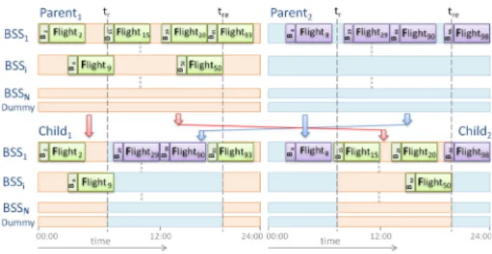
In the 2-point crossover (C2P), two points in time are randomly selected within the time range of the flights, to gen-erate a time window. All flight assignments which lie within this time period, for all of the sorting stations in each solu-tion, are exchanged between the parent solutions, as shown in Fig.8. The flight timings are identical across all solutions, except that the flights in the exchanged region may overlap flights which are not exchanged in the case of some sorting stations. Such overlapping flights in the exchange region are reassigned to other sorting stations where possible; other-wise, they are assigned to the dummy sorting station (i.e. are unassigned).
Whereas in the classic crossover a chromosome is divided into three sections, here the chromosome is divided into 3∗
N sections which correspond to three sections per sorting station.
6.2.2 1-Point crossover
The 1-point crossover (C1P) is a specific case of the above 2-point crossover, where the window extends to the end time of the solution, as shown in the left in Fig.9.
In the presented representation, 1-point crossover is a spe-cial case of 2-point crossover (n =2, number of points),
Fig. 9 Example of 1-point crossover and 1-point serial crossover
where the second point corresponds to the end of the chro-mosome.
6.2.3 n-point crossover
Then-point crossover (CnP) may usen+1 solutions from the population, wherenrefers to the number of cuts. The full time range is divided inton+1 sections, and multiple new solutions are obtained by merging the consecutive sections between the different parents. This recombination may leave some flights unassigned, which may be assigned directly to the dummy sorting station (fictitious sorting station) or an attempt could be made to repair the solution by assigning it to any available sorting station. An extension to 2-point crossover is the n-point crossover which divides the chromo-some into(n+1)∗N which equates ton+1 sections per sorting station.
Usingn-point crossover withn+1 parents can provide up to(n+1)!children. Eiben et al. (1994,1995), Tsutsui and Jain (1998) and Eiben (2003) studied the effect of using multiple parents and multiple crossover points and observed that the increase in the success rate is not merely a consequence of using multiple crossover points, leading to the conclusion that using more parents does increase GA performance.
6.2.4 1-Point serial crossover
The 1-point serial crossover (SC1P) is a different imple-mentation of a crossover operator and may be simpler to understand by representing the problem as a continuous list of BSSs where the crossover cut(s) is in this continuous list, instead of within each BSS as seen in the previously presented crossover operators. The 1-point serial crossover operator is illustrated on the right in Fig.9for the ABSSAP. When the cut(s) has to be determined, a comparison of both parents is made to find the first and last differences in their assignments within the representation, which may be used to restrict the selection of the cut(s). This implementation of a crossover operator is closer to that which is commonly presented in the literature as a 1-point crossover operator, and it is different to that previously introduced in this section.
Figure9shows a simple example where the same parent solutions are used in a 1-point crossover and a 1-point serial crossover side by side. When considering two parents with full assignment, the cut in time (tr s) in the 1-point crossover (C1P) breaks the assigned flights into two groups, each of which contains the same flights for both parents, whereas this is not the case for 1-point serial crossover (SC1P), as shown in Fig.9, where flight ‘3’ is on a different side of the cut in the parents. This means that in the case of SC1P it is necessary to check the assignments after the cut (tr s) from
the second parent to make sure that they have not already been assigned to the first side (from the first parent). Flight ‘3’ is already assigned to the offspring of the first parent and therefore cannot be assigned again to those from the second parent, as shown in Fig.9. So 1-point crossover is simpler to implement than 1-point serial crossover.
Furthermore, this implementation could easily be exten-ded to n points.
Holland (1975) argued that, based on the schema theo-rem to minimise schema disruption, 2-point serial crossover is better than 1-point serial crossover. Although our results show that in some instances 1-point serial crossover provides better solutions than point serial crossover, in general 2-point serial crossover performs best overall. Nevertheless, the schemata theorem is based on a binary representation of the chromosome and binary operators, which differ from the representation and operators presented here, so its applica-tion is of limited interest.
6.3 Combination of operators
Based on how the operator is selected, the types which are of interest are described in the following subsections. It is noted that the operators could be used in complex ways by combining these different types with different parameters. 6.3.1 Probability Single Multi-Operator
The Probability Single Multi-Operator (PSMO) is composed of several sub-operators (which are described in Sect.6), each one of which has a specified probability of being used for the creation of new population members, as shown in Algorithm
3. The combined probabilities across all operators must add up to 1.
As an example, consider a PSMO operator which uses the operators C1P (with a 0.1 probability of being selected) and Multi-Exchange between a Fixed Number of 3 Resources (MEFNR3) (with a 0.90 probability of being selected), which may be represented as PSMO(C1P:10+MEFRN3:90). Given that the total probability must amount to 1, it is not necessary to specify the probability for the last sub-operator, so the representation may also be PSMO(C1P:10+MEFRN3).
The PSMO operator is the one used as base operator in the SSEA experiments presented in Sect.8.
6.3.2 Sequential operator
Considering the way the CGA operates, where a crossover operator may be applied to the parents with a high probability and its children may be further modified by applying a muta-tion operator, the operators may be extended by defining a new operator composed of multiple sub-operators, which are applied sequentially with a given probability (0< p ≤ 1),
Algorithm 3:Probability Single Multi-Operator. Input: Member SelectorSm
Input: Population of solutionsP Input: Operators;Ok∀k∈ [1. . .R]
Input: Probability for operatorspk, 0<pk≤1∀k∈ [1. . .R] andkR=1pk =1
begin
// Initialise
P0← ∅;// empty list of children r=r nd[0. . .1);
k=1;// initialise sub-operator index to first operation p=p1; // Select operator whilek<R and r >pdo k=k+1;// next operator p=p+pk; end
Q←Sm(P,Ok);// get parent solutions for
operator Ok
P0←Ok(Q);// build children by applying
operator to parents
returnP0;// return the obtained children end
Algorithm 4:Sequential Operator. Input: Member SelectorSm
Input: Population of solutionsP Input: Operators;Ok∀k∈ [1. . .R] Input: Probability for each operatorpk,
0<pk≤1∀k∈ [1. . .R] begin
// Initialise
P0←Sm(P,O);// select parents based on
operators // Build children fork=1→Rdo r=r nd[0. . .1); ifr<pkthen Q←P0;// previous children as parent solutions P0←Ok(Q);// applying operator to
the parent solutions
end
i←k+1;// next sub-operator
end
returnP0;// return the obtained children end
as shown in Algorithm 4. This new operator is called the Sequential Operator (SO) herein.
As an example, consider the operators C1P with a selection probability of 1 and the MEFNR3 with a prob-ability of selection of 0.01, which may be represented as SO(C1P:100,MEFNR3:1), where a 1-point crossover is always applied to generate the intermediate children. For these, there is a small probability of 0.01 for application of
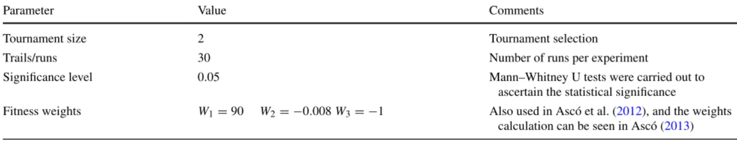
Table 3 Default parameter values
Parameter Value Comments
Tournament size 2 Tournament selection
Trails/runs 30 Number of runs per experiment
Significance level 0.05 Mann–Whitney U tests were carried out to
ascertain the statistical significance
Fitness weights W1=90 W2= −0.008W3= −1 Also used in Ascó et al. (2012), and the weights
calculation can be seen in Ascó (2013)
the MEFNR3 operator in order to generate the final children solutions.
7 General experiments information
A summary of some of the typical values for the different parameters used in the following experiments is shown in Table3.
The data sets used relate to those provided by NATS Ltd. both for 16 December 2009 (H1T091216) and for 1 March 2010 (H1T100301).
The initial solutions were obtained by running the con-structive algorithms presented in Ascó et al. (2010, 2011).
Unless it is mentioned, the parameters presented here refer to all the following experiments for the ABSSAP.
8 Results
The algorithms described are applied to the ABSSAP for different number of BSSs and stands, and their results are compared and analysed in this section for both the data sets obtained from British Airports Authority (BAA)’s website and those provided by NATS Ltd. for Heathrow Airport Lon-don. A fitness function composed of the weighted sum of the different objectives was used to guide the search within the algorithms.
Normality tests were run to identify whether the data could be said to follow a normal distribution, which is a requirement for use of the t-test; otherwise, the Mann–Whitney U test is preferable. Razali and Wah (2011) compared some normality tests and concluded that Shapiro–Wilk is the most powerful normality test. Thus, the Shapiro–Wilk normality test was run for some of the data to ascertain whether the data could be said to be normal, but the data could not be said to follow a normal distribution, the results of which can be seen at Ascó et al. (2013). So Mann–Whitney U tests were carried out to ascertain the statistical significance in the following experiments.
The initial results from experiments executed for BAA’s website data sets for Heathrow Airport London show that
Table 4 CPLEX none default parameter values used for results in Figs.10and12
Parameter Value Comments
NodeFileInd 3 Node file on disc and compressed
WorkMem 128 Memory in MB
NodeSel 1 Best-bound search
VarSel 3 Strong branching
TiLim 3600 and 86400 Time in seconds to end the run
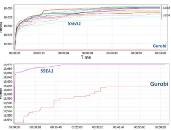
the SSEA presented here provides better solutions than those obtained by CPLEX and Gurobi for the running times con-sidered. These experiments also highlighted the need to have access to a large quantity of Random Access Memory (RAM) given how memory hungry both commercial solvers CPLEX and Gurobi are, making it necessary to run them on a 64bit machine to be able to use more RAM. An initial run with a duration of 1 h was executed, followed by another of 24 h to identify whether the exact method could find the optimum and compare the fittest solution obtained with those obtained by the SSEA. Also the best upper bound obtained from each run was used to help to get an idea of the of the solutions quality obtained from the different algorithms used in the following sections. All the Gurobi parameters used were the default ones with the exception of the time, which was lim-ited to 1 h and 24 h in the two initial runs, and the parameter values used for CPLEX are presented in Table4. Multiple runs were executed to enable the SSEA to take account of the random characteristics of the algorithm with a PSMO composed of 0.2 MEFNR3, 0.2 RMEFNR2, 0.15 C1P and 0.45 DSEMO (only one of the sub-operators will be used at each iteration) with an ES replacement strategy, and the results are shown in Fig.10.
The SSEA quickly improves upon the initial solutions used, reaching solutions fitter than those obtained by Gurobi. Further initial experiments were conducted between the SSEA, CGA and TS with the parameter values as shown in Table5. The results for these experiments, which are pre-sented in Fig.11, also show that SSEA performs better than the other Metaheuristics considered.
Fig. 10 Progress for a 3-pier topology, 48 stands, 78 BSSs and 219 flights (H1T091216)
Table 5 Parameter values used with 30 runs per experiment Algorithm Parameters
Name Value
SSEA Population size 10 and 30 Tournament size 5 Replacement strategy ES
Operator MEFNR3
CGA Population size 10 and 30 Replacement strategy ES
Operator 0.99 C1P and 0.1 MEFNR3
TS Walk size 10
Tabu list size 30
Operator MEFNR3
Fig. 11 Progress for a 3-pier topology, 48 stands, 78 BSSs for 219 flights (H1T091216) and different heuristics
In general, the results obtained show improvements in fit-ness, as shown in Fig.12. Better results were obtained when other Replacement Strategies were used, which are presented in the following sections.
These results show the potential of the SSEA for obtain-ing good solutions even on short runs. It may also be noted that the problem becomes simpler as the number of BSSs
Fig. 12 Average fitness for a 4-pier topology, 46 stands for 194 flights (H1T091216) and different heuristics
increases, especially for the number of BSSs near or bigger than the UMAP, where there are sufficient BSSs to service all the flights while keeping the buffer time intact.
In the next sections, the experiments and their results are presented which were obtained when studying the different parameters part of the SSEA.
8.1 Initial solutions
Experiments were initially conducted to evaluate the influ-ence of the initial population of solutions in reaching better solutions when using good solutions as initial population. The latter have been obtained by applying the constructive algorithms presented in Ascó et al. (2010, 2011), to a data set of 219 flights. The operator used is a PSMO composed of the following sub-operators, each with its own probability of being used; 0.2 for RMEFNRn, 0.2 for Dual Exchange Mutation Operator (DEMO), 0.15 for 1-point crossover and 0.45 for DSEMO, for a population size of ten solutions for a population based algorithms and 78 BSSs (lower than the LMAP). Given that for 78 BSSs full assignment is not pos-sible, use of the DSEMO should help to reach other areas of the search space, thereby improving the solutions obtained. The solutions which do not have maximum assignment may further increase the number of assignments by applying the DSEMO.
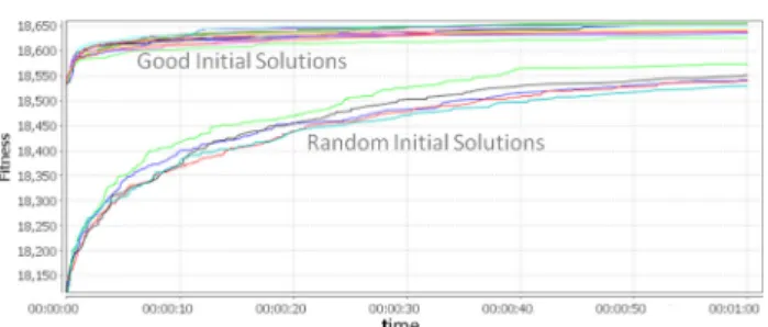
Maximum assignment is achieved where no buffer time is considered, and no restriction is applied as to where the flights may be assigned when ordering the flights by depar-ture time: this is used to generate some of the constructive solutions. The progress of the search is used here for the different initial solutions being considered, in order to illus-trate their contribution in reaching better solutions, as shown in Fig. 13. This provides a view of the Steady-State Evo-lutionary Algorithm with = 1 (SSEA1) behaviour and shows that the algorithm managed to improve on the already good solutions provided as initial solutions, but not as much
Fig. 13 Progress in fitness of solutions when run with and without a initial random population for SSEA1, a 3-pier topology, 78 BSSs, 48 stands and 219 flights (H1T091216)
Fig. 14 Progress in fitness of solutions when run with and without initial random population for Gurobi, a 3-pier topology, 78 BSSs, 48 stands and 219 flights for 1 h
as when the initial solutions are of lower fitness. This is as expected given that there is more leeway to improve on the solutions, but the final fitness of the best solutions is still less than those obtained when good solutions are used. Further-more, the solver Gurobi was run for 1 h, as shown in Fig.14, when no initial solution was provided and when an initial constructive solution (the best of those used for the SSEA1) was used, which showed Gurobi took over 2 min to find a feasible initial solution, when no initial solution is provided. Then quickly improved on this, but still does not manage to reach a fitness such as those reached when a good con-structive initial solution is provided, as is the case with the SSEA1, but at a lower rate. The final solution fitness in both figures shows that SSEA1 provides fitter (better) solutions than those provided by Gurobi, with SSEA1 also improving on Gurobi when no good initial solutions were used.
In summation, the benefits of using good initial solutions in the SSEA are more apparent at short running times, as the differences between fitness decrease as the running time increases, but fitter overall solutions are found when the algo-rithm uses fit good initial solutions. This was also noted when using commercial optimisation applications such as Gurobi and CPLEX.
The mutation operators considered here, with the excep-tion of DSEMO, cannot increase the number of assignments; therefore, solutions which do not have maximum assignment restrict the search space and waste iterations which could otherwise be used to widen the search of the space of
solu-tions potentially improving on those solusolu-tions already found. This can be particularly detrimental if none of the solutions provided are sufficiently fit, i.e. solutions with at least one unassigned flight which is assigned in the optimal solution, as such flights cannot be assigned by these operators. Therefore, when the initial solutions do not have maximum flight assign-ment for the given number of BSSs, the search is restricted to flights already assigned which means low fitness. In these cases, the use of another operator which can increase the number of assignments such as the DSEMO should be used, at least until one or many of the solutions in the population reach maximum flight assignment.
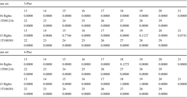
Table 6 shows the statistical fitness significance of the best solution obtained by the SSEA1 with a population size of 30 and a single operator MEFNR3, when using an initial population composed of good solutions obtained from apply-ing the constructive algorithms studied in Ascó et al. (2010,
2011). It is compared with those solutions obtained when the initial population is composed of the 30 fittest solutions from 200 randomly generated solutions (random construc-tive algorithm) for the data set. The empirical results show that the SSEA with good initial solutions provides, in most of the instances considered here, a superior final best solution (statistical fitness significance<0.005) than when the initial population is composed of random solutions.
The algorithms in the study in the following sections use the initial solutions obtained by applying the constructive algorithms which were used in this section and introduced in Ascó et al. (2010, 2011).
8.2 Population size
The effect of the population size (μ) on the results of several of the operators presented in6(Operators) was explored. The parameters used in the experiments are:
1. The data sets used relates to those provided by NATS Ltd. both for 16 December 2009 (H1T091216) and for 1 March 2010 (H1T100301), with both 3-pier and 4-pier topologies, for Heathrow Airport London.
2. Number of BSSs ofN ∈ [13. . .29].
3. The operators used are: C1P, C2P, DSEMO, Multi-Exchange By Pier between a Fixed Number of 3 Resources (MEBPFNR3), MEFNR3 and RMEFNR2. The number of resources (BSSs) considered for the muta-tion operators used was determined by a comparison of the initial results obtained from runs with a population size of 30 for each of the mutation operators.
4. The number of iterations per generationwas initially set to 1.
5. The replacement strategies used are: ES, SUMS, Index Selection with Elitist Selection and a group size of 1
Table 6 Statistical fitness significance for a significance level of 0.05, SSEA1 with fit initial solutions and initial random solutions for the data sets provided by NATS Ltd
Data set 3-Pier
13 14 15 16 17 18 19 20 21 194 flights 0.0000 0.0000 0.0000 0.0000 0.0000 0.0000 0.0000 0.0000 0.0000 H1T091216 22 23 24 25 26 27 28 29 0.0000 0.0000 0.0000 0.0000 0.0000 0.0000 0.0000 0.0000 13 14 15 16 17 18 19 20 21 163 flights 0.0000 0.0686 0.7746 0.0000 0.0000 0.0000 0.1127 0.0000 0.8741 H1T100301 22 23 24 25 26 27 28 29 0.0000 0.0000 0.0000 0.0000 0.0000 0.0000 0.0000 0.0000 Data set 4-Pier
13 14 15 16 17 18 19 20 21 194 flights 0.0000 0.0000 0.0000 0.0000 0.0000 0.1275 0.0000 0.0000 0.0000 H1T091216 22 23 24 25 26 27 28 29 0.0000 0.0000 0.0000 0.0000 0.0000 0.0000 0.0000 0.0000 13 14 15 16 17 18 19 20 21 163 flights 0.0000 0.0000 0.0000 0.0000 0.0000 1.0000 1.0000 0.0000 0.0000 H1T100301 22 23 24 25 26 27 28 29 0.0000 0.0000 0.0000 0.0000 0.0000 0.0000 0.0000 0.0000
(IS1ES) and Index Selection with Stochastic Universal Modified Sampling and group size of 1 (IS1SUMS). 6. Population sizes of μ ∈ {1,5,10,15,30,50,100,200,
500,800,1000,2000} were considered. The algorithm was initially run for population sizes of 15, 30, 50, 100, 200, 500 and 1000. In some instances, the best values appeared at the end of the ranges, which encouraged extending the range of population sizes studied accord-ing to the best population size for each of the operators types.
Regarding the Multi-Exchange Operators, only extra population sizes of 1, 5, 10 were studied, given that these operators are guided mutation operators based on chance and provided better results for the lowest popu-lation sizes initially considered. Nevertheless, given the poor results obtained when using the TS, as shown in Fig.11, it was anticipated that the size of the population should be higher than 1.
In the case of the DSEMO, the results indicated that a high population size was preferred, such that other appropriate population sizes were then considered. The population sizes of 500 and 1000 gave the best results, which was an indication that population sizes between those sizes may potentially be statistically even better. The popula-tion sizes studied were therefore extended to a populapopula-tion size of 800, since a population size of 1000 solutions was statistically significantly fitter in more cases than when using 500 as the population size.
It was observed that the crossover operators performed better for high population sizes as expected, being con-sistently better for the largest population sizes evaluated. Given that a higher population size means a higher run-ning time, a further population size of only 2000 was considered for the crossover operators. If there are too few solutions in a population and given that crossover used the information in the parent solutions, then the opera-tor explores only a small part of the search space. On the other hand, if there are too many chromosomes, the algo-rithm may slow down, as some operations are applied to the full population.
The summary of overall results, when compared using the Mann–Whitney test, is shown in Table7, where italics is used for the values close to those that provided the overall statistically significantly fitter solutions which are presented in black.
With respect to the mutation operators, which are based on a local search, the solutions reached are highly dependent on the individual parent solution, which generally represent small populations. Given that mutation operators require only a parent solution, the population size could range from one solution to many. As the smaller population size would con-sist of one solution, it may be considered that a population size of one should be the best approach from a mutation operator point of view. This relies strongly on the quality of the solution in reaching either a better or optimal
solu-Table 7 Summary of the results of the Mann–Whitney test for significance level of 0.05, different population sizes and replacement strategies
Operator 3-Pier topology 4-Pier topology
Population size Selector Population size Selector
194 flights (16 December 2009)
C1P 2000 IS1SUMS, IS1ES 2000 IS1SUMS, IS1ES
C2P 2000 IS1ES, IS1SUMS 2000 IS1SUMS, IS1ES
DSEMO 800, 1000 IS1ES 500, 800, 1000 IS1ES
MEBPFNR3 10, 5 IS1ES 5, 15 IS1ES
MEFNR3 1, 5 IS1ES 10 IS1ES
RMEFNR2 15 IS1ES 10, 15 IS1ES
163 flights (1 March 2010)
C1P 2000 IS1SUMS, IS1ES 2000 IS1ES, IS1SUMS
C2P 2000 IS1ES, IS1SUMS 2000 IS1ES, IS1SUMS
DSEMO 1000, 800 IS1ES 500 IS1ES
MEBPFNR3 5, 10 IS1ES 5, 10 IS1ES
MEFNR3 10 IS1ES 10, 5 IS1ES
RMEFNR2 15 IS1ES 15, 10 IS1ES
tion, as the fitness does not normally give a clear indication of the solution quality with respect to better solutions in its neighbourhood, which the empirical results corroborate. A solution with lower fitness may be closer to a better or opti-mal solution for the moves performed by the operators used, thus improving the chances that these solutions latter are reached.
In general, crossover operators are expected to benefit from large population sizes, which is corroborated by my results. Given that the crossover operators take advantage of good differences between the parent solutions, the minimum population size required is two solutions. This is the main factor benefiting crossover operators since a large population size normally results in greater diversity within the popula-tion of solupopula-tions. Nevertheless, a higher populapopula-tion size also means a slower algorithm execution time, given that some operations are executed for all members of the population, the processing time of which depends on the number of solu-tions in the population. Additionally, too much diversity may result in a loss of solutions with good building blocks, and have a corresponding detrimental effect on the overall search, the loss of better solutions or the opportunity to reach these better or optimal solutions.
As observed, the population size and operator have an important impact on the algorithm’s performance, but it is not the only factor to consider, as the diversity may also be increased or decreased by changing the selection approaches used, i.e. Replacement Strategies (Sect.1) and the Parent Selector (Sect.2). Elitist Sampling (ES) reduces the diver-sity, as it keeps the solutions with higher fitness, which tends in turn to concentrate the solutions around those with fewer differences, but increases the pressure, whereas Stochastic
Universal Modified Sampling (SUMS, Sect.5) increases the chance of solutions with lower fitness taking part in the pop-ulation of solutions so increasing the diversity. To reduce the ES potential detrimental effect, the Index Selector (ISxy, Sect.5) was designed, implemented and run, the empirical results of which show a better performance than the under-lying Replacement Strategies used, such as ES and SUMS. 8.2.1 Population size for when combined operators are
used
Where different operators have a preference for different pop-ulation sizes, these results may be taken into account when combining operators in order to improve the performance. So when the operator is selected from a pool of operators, randomly for example, its population size preference should be borne in mind so that the parent(s) may be selected within the solutions in the population and within that given preferred size. This assumes that the solutions are ordered in some way. This approach allows better solutions obtained by the other operators with larger preferred population sizes to enter the population of the current operator, potentially increasing the diversity, which it could be considered as a type of migration. In this approach, only the preferred population size is used to select the parent(s) for a given operator.
8.2.2 Run-time results for the different population sizes In this section, they-axis of the graphics is the average exe-cution time for each set of 30 experiments with a different number of BSSs (the number of BSSs is shown in thex-axis). Each graph shows the average results for a given operator and