A Scoping Inquiry into the Potential Contribution of Subjective
Probability Theory, Dempster-Shafer Theory and Possibility Theory
in Accommodating Degrees of Belief in Traveller Behaviour
Research
David A. Hensher Zheng LiInstitute of Transport and Logistics Studies The Business School
The University of Sydney NSW 2006 Australia Tel: +61 2 9114 1824 Fax: +61 2 9114 1722
david.hensher@sydney.edu.au zheng.li@sydney.edu.au
Version: 22 August 2013 (Final 4 December 2013)
To appear in Travel Behaviour and Society
Abstract
There is a small but growing interest in traveller behaviour research on investigating ways to identify and quantify degrees of belief (as subjective probabilities or other propositions) associated with behavioural responses, especially in the context of popular travel choice methods such as stated choice experiments, as a way of adding to our understanding of decision making in real-world contexts that are associated with inevitable risk and uncertainty. This paper reviews three major theories that are not well known in the transportation literature that have been developed in psychology and decision sciences to accommodate belief, namely Subjective Probability Theory, Dempster-Shafer Theory and Possibility Theory. We focus on how degrees of belief are measured in these theories. The key elements of each theoretical approach are compared, including their mathematical properties and evidence patterns. Despite their being few applications to date in transportation, the review promotes the relevance of accounting for degrees of belief in travel choice analysis.
Keyword: belief, degree of belief, Subjective Probability Theory, Dempster-Shafer Theory, Possibility Theory
Acknowledgment: This study is supported by the Australian Research Council Discovery Program Grant DP110100454 titled “Assessment of the commuter's willingness to pay a congestion charge under alternative pricing regimes and revenue disbursement plans”. We also thank two referees and the Becky Loo for comments.
2
Introduction
The economic environment is characterised by unmeasurable uncertainty rather than measurable risk (Knight 1921). If a choice is made under risk, the probability distribution of all possible outcomes is known or can be calculated. Uncertainty is defined as “a quality depending on the amount, type, reliability and unanimity of information, and giving rise to one’s degree of confidence in an estimate of relative likelihoods” (Ellsberg 1961, p.657), under which decision makers have to assess the probabilities of potential outcomes with some degree of vagueness, and rely on their beliefs to make the assessment. A person’s confidence may vary with respect to different propositions, which are the objects of belief, i.e., sets of possible worlds or truth conditions (Huber 2009). For example, she or he is more confident that the bus will arrive at the station on time than that it will be a rainy day tomorrow. The strength of confidence is measured by the degree of belief. Individuals use judgments of numerical probability to represent their degrees of beliefs, which are collected systematically and viewed as an approximation to the degrees of belief implicit in decision making (Idison et al. 2001). The degree of belief of a proposition is typically determined by evidence such as data information, and knowledge, which enable a decision maker to make a judgment and draw a conclusion (Kronprasert 2012).
Given that belief plays a key role in decision making under uncertainty, it is useful to understand belief and to measure degrees of belief. A number of theories have been developed that focus on degrees of belief including Subjective Probability Theory (Ramsey 1931; Savage 1954), Dempster-Shafer Theory (Dempster 1967, 1968; Shafer 1976), and Possibility Theory (Zadeh 1978; Dubois and Prade 1988). The essential difference between the three theories can be best summarized as different mathematical properties (defined in detail in later sections but noting that A and B are any two variables or events or subsets of variables) that are used to account for degrees of belief. Under Subjective Probability Theory, degrees of belief are assumed to be additive (i.e., Pr(A) + Pr(B) = Pr(A∪B) if A∩B = ∅). Dempster-Shafer Theory treats degrees of belief as super-additive (i.e., Bel(A) + Bel(B) ≤ Bel(A∪B)); while Possibility Theory postulates degrees of belief to be sub-additive (i.e., Π(A) + Π(B) ≥ max{Π(A), Π(B)} = Π(A∪B)). The aim of this paper is to provide an overview of these theories, with a focus on how the degree of belief is measured, and to promote the need to incorporate degrees of belief into studies of choice making behaviour in transportation. To date, such theories have attracted little attention by traveller behavior researchers and it can be argued, given the accumulated evidence in psychology and decision sciences, that conditioning choice responses in methods such as stated choice experiments on the ‘believability’ of a hypothetical response reflecting real behaviour may offer a way of weighting such responses by some suitable metric representing the believability or confidence the analyst has in the evidence offered up by respondents in surveys. This is also a way of recognizing and accounting for the confidence that the respondent has in their judgment and choice.
Subjective Probability Theory
The best developed account of degrees of belief is Subjective Probability Theory (Huber 2012). The concept of subjective probability was originally proposed by Ramsay (1931) and
3
further developed by Savage (1954). The entire theory of subjective probability is established around the notion of ‘degree of belief’ (Eriksson and Hάjek 2007). The operational explanation of subjective probability is “the probability of an uncertain event is the quantified measure of one’s belief or confidence in the outcome, according to their state of knowledge at the time it is assessed” (Vick 2002, p.3). Subjective probabilities represent “degrees of belief in the truth of particular propositions”, which reflect individuals’ assessment based on their knowledge and opinions (Ayton and Wright 1994, p.164). Therefore, subjective probabilities actually represent the facts about a decision maker, not about the world, which arise as a response to the failure of frequency-based objective probability theory, when there is the occurrence of uncertain events (Pollock 2006). Anscombe and Aumann (1963) use the horse race as a descriptive example of subjective probability, where individuals made bets according to their subjective probabilities of each horse winning with uncertain consequences. However, risky gambles, such as a roulette wheel, have a finite set of terminal outcomes associated with objective probabilities. Ferrell (1994, p.413) concluded that “subjective probability can enter at any stage of the decision analysis process, implicitly and explicitly as a way of dealing with uncertainty … as the means of quantifying the uncertainties in the models that relate the alternatives to possible consequences.” Decision makers use “subjective probabilities to represent their beliefs about the likelihood of future events or their degree of confidence in the truth of uncertain propositions” (Brenner 2003, p.87). Consequently, to understand the nature of subjective probability can offer important insights into the structure of human knowledge and belief.
Subjective probabilities are constrained by axioms of classical probability theory and follow the laws of probability (Ayton and Wright 1994). Under Subjective Probability Theory, degrees of belief (i.e., subjective probabilities) are additive (Huber 2012). A probability space (S, ℜ, Pr) consists of a set S (i.e., the sample space), a σ-algebra ℜ of subsets of S whose elements are called measurable sets, and a probability function Pr: ℜ → [0, 1], satisfying the following properties:
Pr(X) ≥ 0 for all X
ℜ (1)Pr(S) = 1 (2)
Pr (X1X2 ... Xn...) = Pr(X1) + Pr(X2)+…+Pr(Xn)+…, if theXn’s are
pairwise disjoint members of ℜ (3)
Property (3) is referred to as countable additivity, which can be simplified to finite additivity if ℜ is a finite set:
Pr(X1∪X2) = Pr(X1) + Pr(X2) if X1∩X2 = ∅ (3´)
Ramsey (1931) proposed two ways to identify subjective probability: (i) introspective interpretation, i.e., measuring subjective probabilities by asking respondents; and (ii) behaviourist interpretation, i.e., defining subjective probabilities as a theoretical entity inferred from a choice. The behaviourist interpretation (i.e., subjective probabilities can be estimated from observed preference) was the dominant approach to the elicitation of subjective probabilities before the Ellsberg paradox (Ellsberg 1961).
4
Subjective probabilities elicited from choice (i.e., the behaviourist interpretation) are always calculated based on a linear functional form (essentially all elements of influence are additive in the parameters and the attributes). So, coherent probabilities cannot be obtained, unless an individual’s attitude toward uncertainty is neutral (Baron and Frisch 1994). Given the limitation of the behaviourist interpretation, the introspective interpretation represents a more appealing way to measuring subjective probabilities. Since the 1980s, there have been an increasing number of studies in the area of psychology, behavioural and experimental economics, which directly asked respondents for their probability judgements over uncertain outcomes (see e.g., Kahneman et al. 1982; Heath and Tversky 1991; Fox and Tversky 1998; Wu and Gonzalez 1999; Takahashi et al. 2007). For example, Heath and Tversky (1991) asked respondents to give probability assessments on football predictions and political predictions, and found that uncertainty has an impact on preference. In Wu and Gonzalez (1999), respondents were asked to provide their personal probability assessments on a number of events (e.g., national election and the number of University of Washington football team victories), and their judged probabilities were mapped into decision weights through the non-linear probability weighting function, which they referred to as a two-stage modelling process. Beach and Connolly (2005) defined the elicitation of subjective probabilityas “asking people to give a number to represent their opinion about the probability of an event”.
Based on the behaviourist interpretation, Savage (1954) also suggested that the decision rule under uncertainty is to maximise expected utility based on assigned probabilities (i.e., Subjective Expected Utility Theory (SEUT)). In Savage’s model, subjective probability and utility can be inferred simultaneously from observed preferences. For example, if there is no difference in a subject choosing: (1) winning $10 if tomorrow rains and nothing if not, and (2) an expected win of $5 (winning $10 for a head when tossing a coin (with an objective probability of 0.5)), then we can infer a subjective probability of 0.5. The monetary value of the sure win can be varied so as to identify individuals’ beliefs (subjective probabilities). This normative theory has no distinctive difference between risk and uncertainty, which also suggested that uncertainty may be equivalent to risk for a rational person. Ellsberg’s two-colour example (see Appendix A for details), however, suggests that people are more willing to bet in the situation with known probabilities than without known probabilities. This typical behaviour is referred to as ‘uncertainty or ambiguity aversion’, which in turn highlights the important distinction between risk and uncertainty.
In a transportation context, Hensher et al. (2013) introduced subjective belief in a mixed multinomial logit choice model to identify ex ante support for specific road pricing schemes, such that the evidence in making a choice in a voting model is believable1. The approach is centred on a referendum voting choice model for alternative road pricing schemes in which they incorporated information that accounts for the degree of belief of the extent to which such schemes will make voters better or worse off. They capture the extent of deviation between an obtained belief probability and a perceptually conditioned belief probability, identifying a probability weighting parameter which measures the degree of curvature of the
1 We used the following scale: ‘To what extent do you think that each of these schemes will make you
better (or worse) off? (0=not at all, 100=definitely). Also, ‘In answering this question, how well
informed do you think you are that each of the schemes will make you better off’? 1-6 (1=totally uninformed, 2=strongly uninformed, 3=moderately uninformed, 4=moderately informed, 5=strongly informed, 6=totally informed); and ‘In answering this question, how well informed do you think you are that each of the schemes will make you worse off’?
5
belief weighting function. The overall goodness of fit of the model with embedded belief (adjusted pseudo R2 of 0.353) was significantly better than the model that ignores the role of belief (adjusted pseudo R2 of 0.291). The specific model form is similar to the prospect
theoretic form, with the belief expression being equivalent to the decision weights used in conditioning a parameterised explanatory variable. It is well recognised in the psychology literature (see Tversky and Kahneman 1992) that degrees of belief are implicit in most decisions whose outcomes depend on uncertain events. In quantitative theories of decision making such as subjective expected utility theory or prospect theory, degrees of belief are related to decision weights and are typically identified by either prescribed levels as part of alternatives in a choice experiment or in a more direct manner using a linguistic device such as judgments of numerical probability. Such estimates are often viewed as an approximation to the degrees of belief implicit in decisions or preference revelation (see Fox 1999). It is well recognised that numerical probability judgments are often based on heuristics that produce biases. One of the methods proposed to accommodate some aspects of such potential bias was the idea of a decision weight (Kahneman and Tversky 1979) which accounts for the presence of perceptual conditioning in the way that information reported by decision makers or information offered to decision makers is heuristically processed. Specifically, the value of an outcome is weighted not by its probability but instead by a decision (or belief) weight, w (·), that represents the impact of the relevant probability on the valuation of the prospect. w(.) need not be interpreted as a measure of subjective belief – a person may believe that the probability of a road pricing scheme making them better off is, for example 0.5, but afford this event a weight of more or less than 0.5 in the evaluation of a prospect. See Hensher et al. (2013) for more details.
Under Subjective Probability Theory, the measures of beliefs (i.e., subjective probabilities) are assumed to be additive. However, Ellsberg’s paradox (Ellsberg 1961) revealed evidence which violates this additive assumption (see Ellsberg’s three-colour example summarised in Appendix A). Two theories that relax the additive assumption are introduced in the following sections.
Dempster-Shafer Theory
Like Subjective Probability Theory, a number of alternative theories use either direct judgments or choices between alternatives to quantify degrees of belief. However, they relax the additive assumption (Tversky and Koehler 1994). Among them, the Dempster-Shafer Theory (Dempster 1967, 1968; Shafer 1976) is the most systematic (Mongin 1994; Huber 2012). The Dempster-Shafer (DS) Theory offers an alternative way to assigning likelihoods to events.
Dempster-Shafer Theory has three fundamental elements: frame of discernment (), basic belief assignment (m), and belief (Bel) and plausibility (Pl) functions. The frame of discernment contains all mutually exclusive outcomes of a set S, in which each outcome is called a focal element, representing a proposition that can be either true or false. The power set of S, 2S, contains all possible subsets of the frame of discernment, which is called a body of evidence. Suppose that the set S is {X1, X2, X3}, a body of evidence consists of: {X1}, {X2}, {X3}, {X1, X2}, {X1, X3}, {X2, X3}, X, and ∅. A basic belief assignment (m) defined on a body of evidence2S, is characterised by the following axioms (Ayyub and Klir 2006):
6
m: 2S[0,1] (4)
m(∅) = 0 (5)
m(S) = 1 (6)
m(A∪B) ≥ m(A) + m(B) if A∩B = ∅ (7)
Equation (7) shows that a belief mass (m) under DS Theory is not additive, rather it is a super-additive measure.
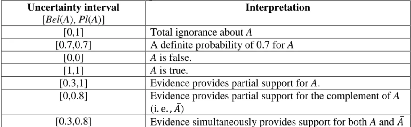
The belief in A is measured by a belief function Bel(A), which is a value in the interval [0, 1]. Bel(A) represents a lower bound on the likelihood of A, and the corresponding upper bound is called the plausibility of A (Pl(A)), both defined on the same body of evidence. Therefore, A is measured by an uncertainty interval [Bel(A), Pl(A)], shown in Figure 1.
Figure 1: Dempster–Shafer uncertainty interval for a proposition
Source: Klein et al. (2002)
Table 1 further explains the meaning of an uncertainty interval. For example, given that there is no direct supporting evidence and no refuting evidence, an uncertainty interval [0,1] suggests total ignorance about A. [0.7,0.7] is an interval with equal support and plausibility, which implies a definite probability of 0.6. [0,0] represents that A is false (or zero probability of occurrence).
Table 1: Interpretation of uncertainty intervals for A
Uncertainty interval
[Bel(A), Pl(A)]
Interpretation
[0,1] Total ignorance about A
[0.7,0.7] A definite probability of 0.7 for A [0,0] A is false.
[1,1] A is true.
[0.3,1] Evidence provides partial support for A.
[0,0.8] Evidence provides partial support for the complement of A (i. e. , 𝐴̅)
[0.3,0.8] Evidence simultaneously provides support for both A and 𝐴̅
Compared to the probability function introduced in the previous section, which assigns a number between 0 and 1 to some subsets of a set, a belief function assigns a number to all
7
subsets of a set (Halpern and Fagin 1992). Moreover, the DS belief function (Bel) is super-additive (i.e., Bel: 2S[0,1]; Bel(A∪B) ≥ Bel(A) + Bel(B) if A∩B = ∅). The theory of DS
belief functions is established under two ideas: (1) obtaining degrees of belief for one question from subjective probabilities for a related question, and (2) combining such degrees of belief when they are based on independent items of evidence. An example to illustrate these ideas is as follows. Peter told me that if he could not use his car to go to work he would take the bus. My subjective probability that Peter is reliable is 0.8, and my subjective probability that he is unreliable is 0.2, given that they are additive. However Peter’s statement, which must be true if he is reliable, is not necessarily false if he is not reliable. Therefore to me, his response alone justifies a 0.8 degree of belief that he would take the bus, but a zero probability of belief (not 0.2 under Subjective Probability Theory) that he would not take the bus given that his response gave me no reason to believe that he would not take the bus. As such, this belief function is described by the 0.8 and zero together2.
The degree of belief of A (Bel(A)) is the sum of all the basic belief assignments given to the proposition P of the set of outcomes where PA and P≠; while the degree of plausibility (Pl(A)) is the sum of all the basic probability assignments of the focal elements P that intersect the focal element A (Malpica et al. 2007).
| ( ) ( ) P P A Bel A m P
(8)
| ( ) ( ) P P A Pl A m P (9)Dempster's rule of combination (see equation 10) offers a mathematical approach to combining two belief functions to produce a new belief function, which is different to the standard operator used in probability theory. Let m1 and m2 be the basic belief assignments from two independent sources. The combined basic belief assignment (m) is given in the following equation (Kronprasert 2012):
, | 1 2 1 2 1 2 , | ( ) ( ) ( ) ( ) ( ) 1 ( ) ( ) X Y X Y A X Y X Y m X m Y m A m X m Y m X m Y (10)where A , the numerator of Equation (10) is the sum of the product of the belief values associated with evidence from two sources supporting Set X, and the denominator is the sum of the product of the belief values associated with all possible combinations of evidence that are not in conflict.
2 The example often cited is from Shafer (1990): Betty told me that a tree limb fell on my car. My subjective
probability that Betty is reliable is 0.9, and my subjective probability that she is unreliable is 0.1, given that they are additive. However Betty’s statement, which must be true if she is reliable, is not necessarily false if she is not reliable. Therefore to me, her testimony alone justifies a 0.9 degree of belief that a tree limb fell on my car, but a zero probability of belief (not 0.1 under Subjective Probability Theory) that no limb fell on my car given that Betty's testimony gave me no reason to believe that no limb fell on my car. As such, this belief function is described by the 0.9 and zero together.
8
Suppose the set X={X1,X2}, and m1 and m2 are the basic belief assignments from two
independent sources: m1({X1})=0.1, m1({X2})=0.4, m1({X1,X2})=0.5,
m2({X1})=0.3, m2({X2})=0.1, m2({X1,X2})=0.6.
The combined basic belief assignment for each focal element is calculated as:
1 1 2 1 1 1 2 1 2 1 1 2 2 1 1 1 1 2 2 1 2 2 1 ( ) ( ) ( ) ( ) ( ) ( ) ( ) 1 [ ( ) ( ) ( ) ( )] m X m X m X m X X m X X m X m X m X m X m X m X 0.1* 0.3 0.1* 0.6 0.5* 0.1 1 (0.1* 0.1 0.4 * 0.3) 0.03 0.06 0.05 0.161 1 (0.01 0.12) 1 2 2 2 1 2 2 1 2 1 1 2 2 2 2 1 1 2 2 1 2 2 1 ( ) ( ) ( ) ( ) ( ) ( ) ( ) 1 [ ( ) ( ) ( ) ( )] m X m X m X m X X m X X m X m X m X m X m X m X 0.4 * 0.1 0.4 * 0.6 0.5* 0.1 1 (0.01 0.12) 0.04 0.24 0.05 0.397 1 (0.01 0.12) 1 1 2 2 1 2 1 2 1 1 2 2 1 2 2 1 ( ) ( ) ( ) 1 [ ( ) ( ) ( ) ( )] m X X m X X m X X m X m X m X m X 0.5* 0.6 1 (0.01 0.12) 0.15 0.345 1 (0.01 0.12)
The measures of belief and plausibility functions are:
1 1 1 1 | | ( ) ( ) 0.161; ( ) ( ) 0.161 0.345 0.506
X X X X X X Bel X m X Pl X m X 2 2 2 2 | | ( ) ( ) 0.397; ( ) ( ) 0.397 0.345 0.742
X X X X X X Bel X m X Pl X m X | | ( ) ( ) 0.345; ( ) ( ) 0.161 0.397 0.345 0.903
X X X X Bel m X Pl m XIn addition to its application in psychology and philosophy (Shafer 1990), the Dempster-Shafer Theory has also been adopted to deal with real-world problems. For example, Tayyebi et al. (2010) used the combination rule of Dempster-Shafer Theory to better choose the landfill site for a city. In this study, three experts’ opinions were asked in terms of weights to weight a number of criteria for landfill site selection including distance from roads, distance from residential areas, distance from water centres and slopes, with the sum of the weights
9
being 1.0 for each expert. The rule of combination then was used to get the final weights. Dempster-Shafer Theory has also been used in mineral exploration. For example, it was applied by Likkason et al. (1997) to integrate geological, geophysical, geochemical, and remotely-sensed data for gold exploration, in which the belief and plausibility measures were used to investigate possible areas for gold. A sensitivity test shows that the final results are robust, given that they are marginally influenced by small changes to the basic probability assignation. The rule of combination (equation 10) has also been used for data fusion in different applications (see e.g., Rottensteiner et al. 2005; Basir et al. 2005; Fan et al. 2006). The Theory has also been applied to model multi-criteria decision making (see e.g., Beynon et al. 2000; Hua et al. 2008).
In the context of transportation, Klein et al. (2002) applied Dempster-Shafer Theory as a data fusion technique to combine traffic incident information from multiple sources including cellular telephones, traffic operation centers and citizens band radio. The database consists of a number of incidents caused by crashes, vehicle blocking lane, unanticipated construction signals or malfunctions. The accuracy rates of the major field data sources are also available, which specifies the percentage of time each data source reported the same incident event as did the highway patrol or city police. For example, a 70% accuracy rate of vehicle blocking lane for a CB radio report describing a vehicle blocking a lane indicates that such a report is correct 70% of the time. 12 incidents were further analysed. For each of them, incident reports were obtained from the data sources, and a probability mass matrix derived from information from each source was created each time an incident was reported. The rule of combination under Dempster-Shafer Theory was used to identify the event with the highest probability as the most likely cause of the incident. By comparing the actual field conditions, this technique delivered an accuracy rate of 75 percent. Zeng et al. (2008) also combined multiple multi-class probability support vector machines using Dempster-Shafer Theory for more accurate traffic incident detection.
Using the belief reasoning method, Kronprasert (2012) compared two public transport alternatives and evaluated their relative degree of support of the goals of the Columbia Pike Transit Initiative project in the Washington Metropolitan Area. For this project, five goals were expected to be achieved by the proposed transit alternatives, namely (i) Improvement of mobility within the corridor; (ii) Enhancement of community and economic development; (iii) Livability and long-term sustainable community; (iv) Development of an integrated multi-modal transport system; and (v) Provision of a safe environment for the citizens and all travel modes. Two alternatives (Bus Rapid Transit (BRT) and streetcar) were evaluated, where the proposed electric-diesel hybrid BRT vehicles are 40 to 60 feet long and can carry approximately 60 to 120 passengers, and the proposed electric streetcar vehicles are 30 to 70 feet long with low-floor and wide doors and they can carry 45 to 190 passengers per vehicle. The method consists of two stages. First, the reasoning map was constructed (see Figure B1 in Appendix B for an example of reasoning map structure), in which the attributes of alternatives which may impact five goals of the project and their causal relations were identified from a number of interviews with experts , and reviews of transit plans and reports, and relevant literature. In the second stage, experts including local and regional transit planners, local experts, and public transit scholars were asked to assign the degrees of belief to the characteristics of alternatives (for example, the degree of belief for the operating speed of Bus Rapid Transit being medium is 0.6) and to the causal relations between variables (for example, if the number of transit station/stops is medium or high, then the travel time reliability is low, with the degree of belief being 0.9) in the proposed reasoning map. The rule
10
of combination is used to aggregate individuals’ beliefs. The degrees of goal achievement for alternative modes are obtained. For each goal, five possible states of outcomes are set, i.e., “Much Higher,” “Higher,” “Same,” “Lower,” “Much Lower”, and “I don’t know”. These relative measures are defined based on the degrees of belief that the streetcar alternative achieves the goals of the project relative to the BRT alternative.
Possibility Theory
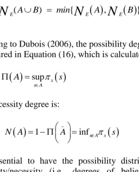
Possibility Theory (Zadeh 1978; Dubois and Prade 1988), based on Fuzzy Set Theory (Zadeh 1965), is another paradigm that accounts for degrees of belief. Possibility Theory is established on set-functions (maxitive and minitive set-functions), in which the degree of belief of a proposition is measured by an interval between a possiblity measure and a necessity measure, representing the degree of belief in an optimistic view and a pessimistic view respectively.
The possibility distribution is the basic object of Possibility Theory. The possibility distribution (x) assigns to each element s in a set S of alternatives a degree of possibility of being the correct description of a state of affairs, and represents what an individual knows about the value of some unknown quantity x ranging on S (Dubois 2006). x(s)=0 for some s means that x=s is impossible; x(s)=1 is considered a normal or unsurprising situation. s,x(s)=1 is the normalisation condition, which claims that there is at least one value regarded as completely possible.
The simplest form of a possibility distribution on the set S is the characterstic function of a subset E of S, i.e., x(s)=1 if xE; x(s)=0 if xE. A possibility function, built from E, is:
1, 0, E if A E A otherwise
(11)E(A)=1 means that xE, xA is possible, as the intersection between set A and set E is not empty. A possibility function satisfies the “maxitivity” axiom (Equation 12).
( ) { , }
E A B max E A E B
(12)
The corresponding necessity measure (NE) is:
1, 0, E if E A N A otherwise (13) and
__ 1 E E N A A (14)Where A is the complement of A. That is, A is necessarily true if and only if ‘not A’ is impossible. NE (neccessity measure) satisfies the “minitivity” axiom (Equation 15).
11
( ) { , }
E A B min E A E B
N
N
N
(15)According to Dubois (2006), the possibility degree of an event A, understood as a subset of S, is measured in Equation (16), which is calculated based on the most plausible value of x in A.
sup x
s A
A s
(16)
The neccessity degree is:
_
1 infs A x
N A A s
(17)
It is essential to have the possibility distribution in order to measure the degrees of possibility/necessity (i.e., degrees of belief under Possibility Theory). Kikuchi and Chakroborty (2006) provided different approaches to developing the possibility distribution. Using travel time variability as an example, a group of travellers are asked to provide the levels of acceptable delay for their commuter trips. Each of them draws a line that represents an individual’s feeling of acceptability on a graph, where the y-axis is the acceptability level between 0 (totally unacceptable) and 1 (totally acceptable), and the x-axis is the delay time (see Figure 2a). Each line starts from the situation that is ‘totally acceptable’ (y=1) without any delay (x=0), and ends at the point where the delay time is totally unacceptable (y=0, and the values of x vary according to the subjects). The combination of the lines drawn by all the subjects (e.g., using the medium line) delivers a representative possibility distribution (see Figure 2b).
Figure 2: Approach 1 to constructing a probability distribution
Source: Kikuchi and Chakroborty (2006)
Another approach is illustrated in Figure 3, in which each subject provides the limit of their acceptable delay, and a horizontal line corresponding to the range of acceptable delay is drawn by the analyst. The analyst stacks all the responses in a same figure (Figure 3a), and joins the rightmost ends of the lines to show the possibility distribution (Figure 3b).
12
Figure 3: Approach 2 to constructing a probability distribution
Source: Kikuchi and Chakroborty (2006)
Henn and Ottomanelli (2006) proposed a model based on Possibility Theory within which to investigate route choice behaviour. Their model follows the specification of Dubois et al. (2001), and the preference index for each route is given as:
inf max 1 ;
i i
v C , where
Ci
is a preference measure on the fuzzy perceived cost for a given situation .When a driver faces alternative routes with prefer indices ( )vi , she or he is assumed to choose route i* with the maximum preference index, that is, vi* max
vi . However, Henn and Ottomanelli did not apply their proposed model to investigate real behaviour, but only provided a numerical application of this model, in which a simple two-route network was assumed, the cost function by the American Bureau of Public Roads was used, and a possibility distribution with values only in [0,1] was considered.Following Henn and Ottomanelli (2006), Ottomanelli et al. (2011) presented a numerical application of Possibility Theory to parking choice, which assumes that the parking user has incomplete information about the supply system, and the perceived cost of each parking alternative (three alternatives were assumed: free parking, illegal parking and charged parking) is represented by a possibility distribution, and the user chooses the one with the lowest perceived cost. The key outcomes are the values of choice probability (Pr) and possibility () for three alternative parking methods under corresponding supply scenarios obtained by varying the dwell time and the controls frequency, given in Table 2, where
Pr Pr Pr 1;
Pr(A B C) ( )A ( )B (C) (A B C) max{ A ,B),B)} 1.
Table 2: Probability (Pr) and possibility (𝜫) for three alternative parking methods under three scenarios
Alternative Scenario 1:
Short dwell time & weak controls
frequency
Scenario 2:
Average dwell time & average controls
frequency
Scenario 3:
Average dwell time & strong controls frequency A:Free parking Pr=0.06;=0.56 Pr=0.19;=0.89 Pr=0.32; =0.89 B:Illegal parking Pr=0.55; =1.0 Pr=0.28; =0.93 Pr=0.10; =0.74 C:Charged parking Pr=0.39; =0.92 Pr=0.53; =1.0 Pr=0.58; =0.58
13
An Illustration of how D-S may be implemented in a travel
choice study
A growing number of travel choice studies ask supplementary questions to elicit how respondents processed specific attributes in a stated choice experiment (e.g., Hensher 2010). The reliability of responses to such questions (e.g., ‘which attributes did you ignore?’ or ‘which attributes did you add up?’) is not without controversy (see Bertrand and Mullainathan 2001), with preliminary evidence suggesting that the willingness to pay (WTP), when the responses to supplementary intention questions are used to condition the treatment of an attribute in model estimation, are sometimes higher and sometimes lower than when processing is excluded. In contrast, the evidence is consistently in the upwards direction when heuristics are tested through the functional specification of non-linear utility expressions (Hensher 2010). So which tendency is ‘correct’? The answer is far from clear; yet the implication on empirical evidence is profound (Hess and Hensher in press).
In this section we focus on the Dempster-Shafer approach to build up an example in some detail of how the method might be used in future traveller behaviour applications, repeating material (in a different way) that was presented above in order to highlight the main elements of the method that need to be translated into an operational model framework. Although we have not tested this example with real data, we would encourage researchers to progress empirical applications within the growing literature on process heuristics and travel choice. (see Hensher 2014 for an overview).
One potentially fruitful way forward is to transform the responses for self-stated processing responses to recognise the potential for error in response. One way worthy of investigation is the belief-function perspective as set out in a previous section. Although not focused on attribute processing per se, the sentiment is aligned. The focus is on the uncertainty that arises because of the lack of knowledge of the true state of nature, where we not only lack the knowledge of a stable frequency (i.e., how can we be sure that the heuristic adopted is stable, as implied by the selected process heuristics), but also we lack the means to specify fully the conditions under which repetitions can be performed (Shafer and Srivastava 1990). The D-S theory of belief functions can be used to assess reliability of evidence that is supplementary to a stated choice experiment, which provides support for the presence or absence of such a variable in situations where the event cannot be treated as a random variable. As set out above, Dempster (1967) introduces belief functions from a statistical perspective in terms of a (frequentist) probability measure from a ‘space of observations’ to a ‘space of interpretations of these observations’ by a ‘point-to-set mapping’ (Dubois & Prade 1988).
We need to find ways in which we can triangulate evidence from various sources, to establish a measure of belief of the evidence offered by an individual on how they processed specific attributes associated with travel choice alternatives. The level of belief on whether the person in question processed an attribute using a specific rule or not, depends on the items of evidence and their credibility. A belief function treatment provides an appealing framework using the two key constructs - belief functions (BF) and plausibility functions (PF). When combined, especially BF and PF, we obtain Dempster’s rule of what we term ‘rule reliability’. We now explain this rule in detail, given it will not be familiar to transportation researchers, in language different to the theoretical exposition above, and suggest (through an
14
example), the nature of data required in future studies to embed the rule reliability measure into the estimation of travel choice models.
The D-S theory of belief functions is similar to probability theory, with one difference. Under probability theory, uncertainty is assigned to the state of nature based on the knowledge of frequency of occurrence. However, under belief functions, uncertainty is assigned to the state of nature or assertion of interest in an indirect way, based on the probability knowledge in another frame, by mapping that knowledge onto the frame of interest. This mapping may not necessarily be one-to-one. To illustrate, suppose we have a variable, A, with n possible mutually exclusive and exhaustive set of values: a1, a2, a3, . . . , an. These values could be alternative ways that an attribute such as a specific congestion charging regime or associated charge is processed, including a simple binary statement of ‘ignored or did not ignore’ the attribute, or ‘added up or did not add up two attributes of a common metric’. Define the frame, = {a1, a2, a3, . . . , an} of discernment for the variable A (i.e., the quality of being able to grasp and comprehend what is obscure). Under probability theory, for such a set, we assign a probability mass, P(ai), to each state ai such that
n i i=1
P(a ) = 1
. However, under the D-S theory of belief functions, uncertainties are assigned in terms of belief masses to not only singletons, but also to all the sub-sets of the frame, and to the entire frame . The entire frame in our example might be a binary setting of ignored (a1) and not ignored (a2) for aspecific attribute associated with an alternative and/or a choice task. (It could also be degrees of attribute relevance (a1, a2 ,…, an) from totally relevant (not ignored) to totally irrelevant
(ignored)).These belief masses define a function called the basic belief mass function (Shafer, 1976). We write a belief mass assigned to a subset B as m(B), where B could be a single element, or a subset of two, a sub-set of three (e.g., degrees of attribute preservation), and so on, or the entire frame, . The sum of such belief masses equals one, i.e., m(B)=1
B
. When
the non-zero belief masses are only defined on the singletons, the belief function reduces to probability theory.
To crystallise this distinction in a numerical example, suppose we were able to determine, from a number of sources, that m(IG) =0.3 and m(NIG)=0 and m(IG,NIG)=0.7. IG stands for ‘the ignore response being a reasonable representation of reality’, and NIG stands for ‘the ignored response being either materially misstated or not reflecting acceptable views of others’.3 The belief function interpretation of these belief masses is that the analyst has 0.3
level of support for 'IG', no support for 'NIG, and 0.7 level of support remains uncommitted which represents ignorance (Dubois and Prade 1988). However, if we had to express the above judgment in terms of probabilities, we would assign P(IG) = 0.3 and P(NIG) = 0.7, which implies that there is a 70 percent chance that the response to the question is ‘materially misstated or does not reflect acceptable views of others’. However this is not what the analyst’s judgment is; they have no information or evidence that ignoring an attribute is materially misstated. Simply knowing that the response appears to be reasonable, compared to the predicted values based on the average views of others, including additional information obtained from the specific individual, provides no evidence that the response to the question
3 Information to gauge the reliability of stated self-intentions could be sought from the very same person along
similar lines to supplementary questions used in reducing the hypothetical bias gap in WTP. An example is a
certainty scale question, as suggested by Johannesson et al. (1999), on a scale 0 (very unsure) to 10 (very sure), to indicate how sure or certain the respondent is that they would actually chose that route (or not at all) at the indicated price and travel time.
15
on whether an attribute is ignored is materially misstated. It only provides some level of support that the subjective response is accurately stated. Formally, the Belief Function is defined as follows: The belief in B, Bel(B), for a subset B of elements of a frame, , represents the total belief in B, and is equal to the belief mass, m(B), assigned to B plus the sum of all the belief masses assigned to the set of elements that are contained in B. In terms of symbols: Bel(B) =
C B
m(C)
(equation 8). The Plausibility Function Pl(B) (equation 9) represents the maximum belief that could be assigned to B, given that all the evidence collected in the future support B. For example, for two independent items of evidence pertaining to a frame of discernment, , we can write the combined belief mass for a sub-set B in using Dempster’s rule:1 2 C1 C2 = B m(B) = m (C1)m (C2)/K
, (18a) C1 C2 = 1 2 K = 1 m (C1)m (C2)
(18b)The symbols m1(C1) and m2(C2) determine the belief masses of C1 and C2, respectively, from the two independent items of evidence represented by the subscripts. K is a re-normalisation constant. The second term in K represents the conflict between the two items of evidence (Shafer 1976); the two items of evidence are not combinable if the conflict term is 1. Let us bring this framework together in an example. Suppose we have the following sets of belief masses obtained from two independent items of evidence related to the accurate representation of whether an attribute such a congestion charging regime (as distinct from the actual charge) is ignored (IG) or not (NIG):
Evidence 1: m1(IG) = 0.3, m1(NIG) = 0.0, m1({IG, NIG}) = 0.7, Evidence 2: m2(IG) = 0.6, m2(NIG) = 0.1, m2({IG, NIG }) = 0.3.
The re-normalisation constant for the above case is:
K = 1 – [m1(IG)m2(NIG) + m1(NIG)m2(IG)] = 1 – [0.3*0.1 + 0.0*0.6] = 0.97.
Using Dempster’s rule (18a), the combined belief masses for ‘IG’, ‘NIG’, and {IG, NIG} are: m(IG) = [m1(IG)m2(IG) + m1(IG)m2({IG, NIG }) + m1({IG, NIG })m2(IG)]/K
= [0.3*0.6 + 0.3*0.3 + 0.7*0.6]/0.97 = 0.69/0.97 = 0.71134,
m(NIG)=[m1(NIG)m2(NIG)+m1(NIG)m2({IG,NIG})+m1({IG,NIG })m2(NIG)]/K = [0.0*0.1 + 0.0*0.3 + 0.7*0.1]/0.97 = 0.07/0.97 = 0.072165,
m({IG, NIG }) = m1({IG, NIG })m2({IG, NIG })/K = 0.7*0.3/0.97 = 0.21/0.97 = 0.216495. (19)
The combined beliefs and plausibilities that attribute processing is not misstated are: Bel(IG) = m(IG) = 0.71134, and Bel(NIG) = m(NIG) = 0.072165, (20a) Pl(IG) = 1 – Bel(NIG) = 0.927845, and Pl(NIG) = 1 – Bel(IG) = 0.28866.(20b)
The choice model, for each individual observation, can have each attribute discounted by the ‘plausibility factors’ Pl(IG) (=0.927845) and Pl(NIG) (=0.28866). This might be, for example, a decomposition of a random parameter in a generalised mixed logit (GMX) model or introduced as a latent construct in a latent variables mode (e.g., Hess and Hensher 2013).
16
These plausibility factors would be applied to all observations, based on evidence obtained from supplementary questions. The challenge for research into choice on congestion charging schemes, for example, is to identify a relevant set of questions posed to the respondent and other influencing agents that can be used to quantify evidence, suitable to deriving the belief and plausibility functions for each respondent.
Krantz (1991) and Tversky and Koehler (1994) show that D-S’s model is most suitable for judgments of evidence strength than for judgments of probability. The judgments of evidence strength is the very role that the plausibility function plays in the context of specifying the way that a specific attribute is processed in the context of stated choice experiments. We are not using the belief theory to establish probabilities of outcomes, since that is accommodated though the choice model. For example, if we have seven attributes (x1 to x7), of which the
first two have a common metric (e.g., running cost and toll cost), the next two have a common metric (e.g., free flow and congested time), and the next three define the congestion scheme (charge, regime and revenue disbursement), we might have a number of ways in which we can structure questions suitable for establishing how each specific attribute is processed (in the context of how the package of attributes is processed). This is crucial in the design, and hence acceptability, of congestion charging schemes. There are a number of possible ways of evaluating an attribute in arriving at a decision on how it will be processed in the context of a choice task. These might be based on five items of evidence in relation to the processing of x5, thecongestion charge: (i) ignored or not, (ii) added up with another
common-metric attribute (e.g., congestion charge and running cost), (iii) accepted subject to a threshold level of a congestion charge, (iv) the actual charging regime such as cordon charge which is less ambiguous than a distance based charge, and (v) how revenue raised is disbursed:
E_ = E(x5): I evaluated only x5 in deciding what role x5 plays
E_ = E(x5,x6); E(x5,x6); E(x5,x7);…E(E(x5,x6,x7): I evaluated x51 from a subset of attributes
offered
E_: = E(x5,x6): I evaluated x5 in the context of attributes that have a common metric with x5
E_: = E(x5+x1,x3+x4): I evaluated x5 by adding up attributes that have a common metric
E_: = E(x1 to x7): I evaluated every attribute in deciding what role x5 plays.
For each of these candidate heuristics, the analyst might ask, in a context of whether the congestion charge was ignored or not: ‘Please allocate 100 points between the three possible ways you might respond to reflect your assessment of how you believe you used each of the processing rules in determining the role of the congestion charge :
I definitely ignored the congestion charge _______ I did not fully ignore, or fully not ignore, the congestion charge _______ I definitely did not ignore the congestion charge _______
These heuristics may be randomly assigned to each respondent or all might be assigned to each respondent (in a randomised order). There are some clear disadvantages of assigning all heuristics to each respondent, yet this may be necessary in order to obtain the required data to calculate a plausibility expression. A possibility is to initially get the respondent to order the heuristics in order of applicability (in the example above this is a rank from 1 to 5, where 1 = most applicable), followed by a response to the 100 point allocation question. If the focus is on whether a congestion charge was ignored or not, then we might identify the following evidence:
17
E_: E_(IG) = 0.4, E_(NIG) = 0.2, E_({IG,NIG}) = 0.4 rank = 4 E_: E_ (IG) = 0.4, E_ (NIG) = 0.3, E_ ({IG,NIG}) = 0.3 rank = 3
E_: E_ (IG) = 0.5, E_ (NIG) = 0.3, E_ ({IG,NIG}) = 0.2 rank = 2 (21) E_: E_ (IG) = 0.3, E_ (NIG) = 0.3, E_ ({IG,NIG}) = 0.6 rank = 5
E_: E_ (IG) = 0.5, E_ (NIG) = 0.2, E_ ({IG,NIG}) = 0.3 rank = 1
The responses to (21) can be fed into equation (19) to obtain the belief and plausibility values in (20a) and (20b), interacted with each attribute in the generalised mixed logit model (equation 22) through zi and hi (see below) to account for the attribute processing strategy of
each respondent at an alternative and at a choice set level. This model form is detailed in Greene and Hensher (2010).
, 1 , exp( ) ( , , ) exp( ) it it j ir it ir J j it j ir P j x X x , , 1 1 1 1 1 log N log R Ti Jit ( , , )dit j it ir i r t j L P j R
X (22)βir = σir[β + Δzi ] + [γ + σir(1 – γ)] Γvir, ir = exp[-2/2 + δ′hi + τwir], vir and wir = the R simulated draws on vi and wi, ditj = 1 if individual i makes choice j in choice situation t and 0 otherwise. σi is the individual specific standard deviation of the idiosyncratic error term, hi is a set of L characteristics of individual i that may overlap with zi, δ are parameters in the observed heterogeneity in the scale term, wi is the unobserved heterogeneity standard normally distributed, is a mean parameter in the variance, is the coefficient on the unobserved scale heterogeneity, and is a weighting parameter that indicates how variance in residual preference heterogeneity varies with scale, with 0 < < 1.
Conclusions
This paper has reviewed Subjective Probability Theory, Dempster-Shafer Theory and Possibility Theory, and his/her roles in accommodating belief and measuring degrees of belief. The characteristics of the three theories are summarised. To be able to capture belief and measure degrees of belief is recognised in the broad decision theory literature as important in understanding decision making under uncertainty. In the context of transportation, for example, travel time variability due to unpredictable fluctuations in traffic demand and supply is inherent to transport systems, and results in multiple possible travel times (arriving early, on time and late) for a future trip. However, this travel time distribution is not available or unclear to a traveller, and hence she or he has to assess the probabilities of potential outcomes based on their belief. The same logic, for example, applies to crowding (and getting a seat) in public transport.
Different mathematical properties are used to account for degrees of belief under the three theories. Under Subjective Probability Theory, degrees of belief are assumed to be additive (i.e., Pr(A) + Pr(B) = Pr(A∪B) if A∩B = ∅). Dempster-Shafer Theory treats degrees of belief as super-additive (i.e., Bel(A) + Bel(B) ≤ Bel(A∪B)); while Possibility Theory postulates degrees of belief to be sub-additive (i.e., Π(A) + Π(B) ≥ max{Π(A), Π(B)} = Π(A∪B)). The evidence pattern in Subjective Probability Theory is exclusive evidence (see Figure 4a in which each evidence (E) points to one outcome only (mutually exclusive)), while Possibility Theory is nested evidence (see Figure 4b in which E3 is a nested evidence to E4, E2 and E1);
18
while the Dempster-Shafer Theory is capable of handling the mix of all patterns of evidence (Kronprasert 2012). Other unique characteristics of three theories are summarised in Table 3.
Figure 4: Exclusive and nested evidence patterns Source: Kronprasert (2012)
Table 3: Characteristics of Subjective Probability Theory, Dempster-Shafer Theory, and Possibility Theory
Characteristics Subjective Probability Theory Dempster-Shafer Theory Possibility Theory Element xX xX xX Function Pr: Probability function
m: Belief assignment Possibility distribution
Evidence pattern Exclusive Mixed Nested
Degree of belief measure
Subjective probability
Belief & Plausibility Possibility & Necessity
Property Additive Super-additive Sub-additive
With rare exception (as cited in this paper), measures of degree of belief have been overlooked in the transportation literature, and we have found very few transportation studies which have applied these theories to capture belief and measure degrees of belief when modelling travel choices. This review highlights the appeal of accommodating degrees of belief, and provides important inputs for future transportation studies to incorporate degrees of belief into a better understanding of choice behaviour. We have set out an extended example of how the D-S method might be integrated into travel choice models.
In addition to a focus on travel choice, the growing interest in understanding how we can increase buy-in from stakeholders to important policy issues such as road pricing reform, climate change and social inclusion, suggests a role for belief. Broadly interpreted, this includes evidence on the extent (e.g., subjective probability) to which a specific reform package will make a voter better off, supplemented by information to reveal the extent to which a voter believes that they are informed or uninformed that the road pricing reform package will make them better or worse off.
19
There is no conclusive evidence to suggest that one approach has necessarily delivered the greater behavioural insights over another approach. What would be an important future research activity would be a controlled comparison of the three approaches in terms of key behavioural outputs such as overall predictive power (with hold out samples), elasticities and willingness to pay estimates.
A key challenge in implementing these theories is the collection of relevant data. We have found in a recent study (Hensher et al. 2013) that the specification of the required data is a relatively demanding task, and involves survey questions that are typically absent from transportation surveys, including the more advanced stated choice surveys. As an example, we reproduce a screen (Figure 5) from the Hensher et al. (2013) road pricing study that was considered by respondents as the most ‘difficult’ feature of the survey. Extensive training of interviewers in a face to face data collection setting was essential in order to ensure that respondents understood these questions.
20
21
Appendix A
Table A1: Ellsberg paradox: three-colour balls 30 balls 60 balls
Red Black Yellow
A1 $100 0 0
B1 0 $100 0
A2 $100 0 $100
B2 0 $100 $100
Ellsberg paradox: three-colour balls. An urn contains 90 balls of three different colours (three states): 30 red balls and 60 balls either black or yellow (however the exact number of black (or yellow) balls is unknown). Respondents4 were asked to draw a ball from the urn
without looking and were provided with two choices: between: (A1) win $100 if the ball drawn is red (and nothing if it is black or yellow) and (B1) win $100 if the ball drawn is black (and nothing if it is red or yellow); between: (A2) win $100 if the ball drawn is either red or yellow (and nothing if it is black); (B2) win $100 if the ball drawn is either black or yellow (and nothing if it is red). The majority of respondents favoured A1 over B1, and B2 over A2. However, based on the sure-thing principle of SEUT, if individuals prefer A1 over B1, they should also favour A2 over B2, and vice versa. Since the consequence of drawing a yellow ball is the same for the choice between alternatives A1 and B1 (i.e., 0) and same for the choice between A2 and B2 (i.e., $100), the state of a yellow ball (which provides the same consequence for A1 and B1 in one choice and A2 and B2 in another choice) should have no impact on an individual’s two choices (A1 or B1; A2 or B2) (i.e., state independent); while the consequence of drawing a red ball or a black ball is the same for alternative A1 in the first choice and alternative A2 in the second choice; and also the same for alternative B1 in the first choice and alternative B2 in the second choice. Therefore, under SEUT, if A1 is preferred over B1, then A2 should also be preferred over B2 (i.e., A1>B1 and A2>B2). However, Ellsberg’s finding (A1>B1 and B2>A2) violates the sure-thing principle, which assumes subjective probabilities are linear-additive.
For the choice between A1 and B1, it is less ambiguous to draw a red ball (a win for A1) than to draw a black ball (a win for B1). For the choice between A2 and B2, the ambiguity is associated with drawing a yellow ball (a win for A2); while either a black or yellow ball would yield a win for B2 (which is similar as drawing a red ball out of 30 red balls). Hence the pattern found by Ellsberg’s paradox (A1>B1 and B2>A2) suggests that people prefer more precise knowledge of probabilities. This preference was also revealed in Ellsberg’s two-colour paradox (Ellsberg 1961).
Ellsberg paradox: two-colour balls. There are two urns: urn I has 50 red balls and 50 black balls, and urn II also contains 100 balls, however in which the exact numbers of black (b) balls and red (r) balls are unknown. The task is to guess the colour of a ball drawn from either urn I or urn II. You will win a prize if the guess is correct. Ellsberg found that people prefer to draw a red (or black) from urn I with the known probability than a black (or red) from urn II without the known probability; while there is no significant difference between drawing a ball from either urn I and urn II. That is, the colour itself has no impact on the choice, while
22
the preference is dependent on the ambiguity of the probabilities. When drawing a red or black ball from urn I, the likelihood is more direct (i.e., 0.5: 50 red balls and 50 black balls) relative to from urn II where people need to personally judge the possible combination of red and black balls.
Appendix B
Figure B1: Reasoning map for Goal 3 “Livability and Sustainable Community” Source: Kronprasert (2012)
References
Anscombe, F.J., and Aumann, R.J. (1963) A definition of subjective probability, Annals of Mathematical Statistics, 34(1), 199-205.
Ayton, P. And Wright, G. (1994) Subjective probability: what should we believe?, in Wright, G. and Ayton, P. (eds.) Subjective Probability, John Wiley & Sons, Chichester, UK, 163-184.
Ayyub,B. and Klir, G (2006)Uncertainty Modeling and Analysis in Engineering and the Sciences, Chapman and Hall/CRC, Baton Rouge, Florida.
Baron, J. and Frisch, D. (1994) Ambiguous probabilities and the paradoxes of expected utility, in Wright, G. and Ayton, P. (eds.) Subjective Probability, John Wiley & Sons, Chichester, UK, 273-294.
Basir O., Karray F. and Zhu H. (2005) Connectionist-based Dempster–Shafer evidential reasoning for data fusion, IEEE Transactions on Neural Networks, 16(6), 1513-1530.
23
Beach, L.R. and Connolly, T. (2005) The Psychology of Decision Making, Sage Publications, California, USA.
Beynon, M., Curry, B., and Morgan, P. (2000) The Dempster-Shafer theory of evidence: an alternative approach to multicriteria decision modelling, Omega, 28(1), 37-50.
Brenner, L.A. (2003) A random support model of the calibration of subjective probabilities, Organizational Behavior and Human Decision Processes, 90(1), 87–110.
Dempster, A.P. (1967) Upper and lower probabilities induced by a multivalued mapping, Annals of Mathematical Statistics, 38(2), 325-339.
Dempster, A.P. (1968) A generalization of Bayesian inference, Journal of the Royal Statistical Society. Series B, 30(2), 205-247.
Dubois, D. (2006) Possibility theory and statistical reasoning, Computational Statistics & Data Analysis, 51(1), 47-69.
Dubois, D. and Prade, H. (1988) Possibility Theory, Plenum Press, New York.
Dubois, D., Prade, H. and Sabbadin, R. (2001) Decision theoretic foundations of qualitative possibility theory, European Journal of Operational Research, 128(1), 459–478.
Ellsberg, D. (1961), Risk, ambiguity and the Savage axioms, The Quarterly Journal of Economics, 75(4), 643–669.
Eriksson, L. and Hάjek, A. (2007) What are degrees of belief?, Studia Logica, 86, 183–213. Fan X., Huang H. and Miao Q. (2006) Agent-based diagnosis of slurry pumps using
information fusion, Proceedings of the International Conference on Sensing, Computing and Automation, 1687-1691.
Ferrell, W.R. (1994) Discrete subjective probabilities and decision analysis: elicitation, calibration and combination, in Wright, G. and Ayton, P. (eds.) Subjective Probability, John Wiley & Sons, Chichester, UK, 411-451.
Fox, C. R. (1999) Strength of evidence, judged probability, and choice under uncertainty, Cognitive Psychology, 38, 167–89.
Fox, C.R. and Tversky, A. (1998) A belief-based account of decision under uncertainty, Management Science, 44, 879–895.
Greene, W.H. and Hensher, D.A. (2010) Does scale heterogeneity across individuals matter? A comparative assessment of logit models, Transportation, 37 (3), 413-428.
Halpern, J.Y. and Fagin, R. (1992) Two views of belief: belief as generalized probability and belief as evidence, Artificial Intelligence, 54(3), 275-317.
Heath, C. and Tversky, A. (1991) Preference and belief: Ambiguity and competence in choice under uncertainty, Journal of Risk and Uncertainty, 4, 5–28.
Henn, V. and Ottomanelli, M. (2006) Handling uncertainty in route choice models: from probabilistic to possibilistic approaches, European Journal of Operational Research, 175(3), 1526-1538.
Hensher, D.A. (2010): Attribute Processing, Heuristics and Preference Construction in Choice Analysis. in Hess, S. and Daly, A. (eds.) Choice Modelling, Emerald Press, UK, Chapter 4.
Hensher, D.A. (2014) Attribute processing as a behavioural strategy in choice making, in Hess, S. and Daly, A.J. (eds.), Handbook of Discrete Choice Modelling, Edward Elgar, UK,
Hensher, D.A., Rose, J.M. and Collins, A. (2013) Understanding buy in for risky prospects: incorporating degree of belief into the ex ante assessment of support for alternative road pricing schemes, Journal of Transport Economics and Policy, 47 (3), 453-73.
Hess, S. and Hensher, D. A. (2010) Using conditioning on observed choices to retrieve individual-specific attribute processing strategies, Transportation Research Part B, 44(6), 781-90.
24
Hess, S. and Hensher, D. A. (2013) Making use of respondent reported processing information to understand attribute importance: a latent variable scaling approach, (Presented at 2012 Transportation Research Board Annual Conference, Washington DC) Transportation, 40 (2), 397-412.
Hua, Z., Gong, B., and Xu, X. (2008) A DS-AHP approach for multi-attribute decision making problem with incomplete information, Expert Systems with Applications, 34(3), 2221-2227.
Huber, F. (2009) Belief and degrees of belief, in Huber, F. and Schmidt-Petri, C. (eds.), Degrees of Belief, Springer, Dordrecht, 1–33.
Huber, F. (2012) Formal representations of belief, in Zalta, E.N. (ed.), The Stanford Encyclopedia of Philosophy, http://plato.stanford.edu/archives/fall2012/entries/formal-belief.
Idison, L.C., Krantz, D.H., Osherson, D., and Bonini, N. (2001) The relation between probability and evidence judgment: an extension of support theory, The Journal of Risk and Uncertainty, 22(3), 227–249.
Johannesson, M., Blomquist, G., Blumenschien, K., Johansson, P., Liljas, B. and O’Connor, R. (1999): ‘Calibrating hypothetical willingness to pay responses’, Journal of Risk and Uncertainty, 8, 21-32.
Kahneman, D., and Tversky, A. (1979) Prospect theory: an analysis of decision under risk, Econometrica, 47(2), 263-92.
Kahneman, D., Slovic, P. and Tversky, A. (1982) Judgment under Uncertainty: Heuristics and Biases, Cambridge University Press, Cambridge, UK.
Kikuchi, S. and Chakroborty, P. (2006) Place of possibility theory in transportation analysis. Transportation Research Part B, 40(8), 595-615.
Klein, L. A., Yi, P., and Teng, H. (2002) Decision support system for advanced traffic management through data fusion. Transportation Research Record: Journal of Transportation Research Board No. 1804, 173-178.
Knight, F. (1921) Risk Uncertainty and Profit, Houghton Mifflin, Boston.
Krantz, D.H. (1991): ‘From Indices to Mappings: The representational Approach to Measurement’, in Frontiers of Mathematical Psychology: Essays in Honour of Clyde Coombs, Brown, D, & Smith, E. (eds.), Springer Verlag, 1-52.
Kronprasert, N. (2012) Reasoning for Public Transportation Systems Planning: Use of Dempster-Shafer Theory of Evidence, PhD Dissertation, Virginia Polytechnic Institute and State University.
Likkason, O. K., Shemang, E. M., & Suh, C. E. (1997) The application of evidential belief function in the integration of regional geochemical and geological data over the Ife-Ilesha goldfield, Nigeria, Journal of African Science, 25(3), 491–501.
Malpica, J. A., Alonso, M. C., and Sanz, M. A. (2007) Dempster-Shafer theory in geographic information system: A survey, Expert Systems with Applications, 32(1), 47-55.
Mongin, P. (1994) Some connections between epistemic logic and the theory of nonadditive probability, in Humphreys, P.W. (ed.) Patrick Suppes: Scientific Philosopher, Kluwer, Dordrecht, Netherlands, 135-171.
Ottomanelli, M., Dell’Orco, M., and Sassanelli, D. (2011) Modelling parking choice behaviour using Possibility Theory, Transportation Planning and Technology, 34(7), 647–667.
Pollock, J.L. (2006) Thinking about Acting: Logical Foundations for Rational Decision Making, Oxfird University Press, New York, USA.
Ramsey, F.P. (1931) Truth and probability, In Braithwaite R.B. (ed.) The Foundations of Mathematics and Other Logical Essays by F.P. Ramsey, Harcourt, Brace, New York, 158-198.